Novel Soliton Solutions of the Fractional Riemann Wave Equation via a Mathematical Method

Abstract

The Riemann wave equation is an intriguing nonlinear equation in the areas of tsunamis and tidal waves in oceans, electromagnetic waves in transmission lines, magnetic and ionic sound radiations in plasmas, static and uniform media, etc. In this innovative research, the analytical solutions of the fractional Riemann wave equation with a conformable derivative were retrieved as a special case, and broad-spectrum solutions with unknown parameters were established with the improved (G’/G)-expansion method. For the various values of these unknown parameters, the renowned periodic, singular, and anti-singular kink-shaped solitons were retrieved. Using the Maple software, we investigated the solutions by drawing the 3D, 2D, and contour plots created to analyze the dynamic behavior of the waves. The discovered solutions might be crucial in the disciplines of science and ocean engineering.

1. Introduction

Over the last few decades, numerical and exact solutions to nonlinear partial differential equations (NLPDEs) [1,2] have appeared to be of great interest to many scholars due to the amazing popularity of nonlinear sciences and engineering. Recently, the stability analysis of nonlinear fractional partial differential equations (NLFPDEs) has played an important role in the field of solitary wave theory. Analytical solutions of NLFPDEs are crucial in applied nonlinear research. Moreover, the structures of natural phenomena are better described by fractional-order differential equations than by integer-order differential equations. The use of analytical techniques to find traveling wave solutions to NLFPDEs [3,4,5] can explain the physical behavior of related real-world problems more effectively. Researchers have increasingly concentrated on analytical and numerical solutions to NLFPDEs [6,7,8,9,10,11] with the help of computer science and symbol-based software. Numerous robust computational techniques have been developed in the literature to explore the various types of exact solutions of NLFPDEs, such as the extended rational sinh–cosh method [12], extended tanh–coth method [13], exp-function method [14,15], fractional Riccati expansion method [16], generalized Kudryashov approach [17], enhanced and generalized (G’/G)-expansion scheme [18,19], and Painleve Property [20].

Few years ago, Wang et al. [21] developed the (G’/G)-expansion method, a popular, direct, and brief technique for finding exact traveling wave solutions. Different modifications of the (G’/G)-expansion method have been developed by different researchers, but the improved (G’/G)-expansion method is also one of the most reliable, effective, and consistent methods used by different scholars to extract traveling wave solutions of NLPDEs. For instance, Islam et al. [19] presented the nonlinear dynamics of magnetic soliton solutions, several soliton solutions of a nonlinear model were constructed by Yokus et al. [22] by means of the (G’/G 1/G)-expansion method, some researchers obtained the dynamical and physical nature of a few novel and accurate trigonometric, hyperbolic, and rational solitary wave solutions with the help of Atangana’s conformable differential operator by using an efficient (G’/G)-expansion method [23,24,25], and Younis et al. [26] constructed solitary wave solutions to the Schr$\ddot{\mathrm{o}}$dinger-Poisson system with the help of the (G’/G)-expansion method.

The characteristics of the improved (G’/G)-expansion method boosted our interest in a notable and suitable model for the Riemann wave equation (RWE), which is associated with superconductivity, plasma electrostatic waves, and ion–cyclotron wave electrostatic potential in a centrifugally inhomogeneous plasma. Consider a type of generalized $\left(2+1\right)-$dimensional breaking soliton equation (BSE) [27]:

$$v_t+a{v}_{xxx}+b{v}_{xxy}+cv{v}_x+dv{v}_y+e{v}_x{\partial }_x^{-1}{v}_y=0,$$

(1)

where $a, b, c, d,$ and $e$ are real parameters and ${\partial }_x^{-1}$ [28] is the inverse operator of $\frac{\partial }{\partial x}$. By using the Painleve property, there are different choices for the values of real parameters. The spectral parameters used in the Lax representations demonstrate breaking behavior, which is a distinctive characteristic of this family of equations. As a consequence of the spectral values the solutions evolve into multivalued functions. As a result, the $\left(2+1\right)-$dimensional breaking soliton equations (BSEs) [27]

$$\begin{array}{c}{v}_t+a v_{xxx}+b v_{xxy}+cv{v}_x+dv{w}_x+ew{v}_x=0, \hfill \\ \hfill v_y=w_x\hfill \end{array}$$

(2)

with different overlapping solutions were developed, and they propagate along the $y-\mathrm{axis}$while interacting with a long wave traveling toward the $x-axis$. The Riemann wave equation [29]

$$\begin{array}{c}{v}_t+\beta v_{xxy}+nv{w}_x+mw{v}_x=0, \hfill \\ \hfill v_y=w_x,\hfill \end{array}$$

(3)

is a type of generalized $\left(2+1\right)-$dimensional BSE. Moreover, this $\left(2+1\right)$-dimensional BSE is associated with the Ablowitz–Kaup–Newell–Segur (AKNS) hierarchy. In addition to this, these equations have a wide range of applications for the propagation of tidal and tsunami waves in the ocean. These equations also represent the turbulent state by using a mixture of Whistler wave packets and random phases with a finite amplitude. A magnetic sound wave is dampened because the Whistler turbulence’s interaction with it dampens a plasma’s electrostatic wave [27]. Scholars and researchers have recently been very concerned with finding RWE solutions by using various methods. The Wronskian method was used to extract rational and periodic solutions of a $\left(2+1\right)-$dimensional BSE by Hong-hai et al. [30], soliton solutions to the RWE were derived by Barman et al. by using the extended tanh-function technique [27], Barman et al. [29] used the generalized Kudryashov method to establish traveling wave solutions, Roy et al. [31] evaluated exact bright–dark solitary wave solutions with the aid of the generalized (G’/G)-expansion method, and the generalized exponential rational function approach was utilized by the authors of [32] to evaluate RWE solutions that simulated the construction, breaking, and interaction of waves that resulted from any peripheral influence on the ocean envelope.

Taking the prior analysis into account, consider a Riemann wave equation of fractional order:

$$\begin{array}{c}{v}_t^{\alpha }+\beta v_{xxy}+nv{w}_x+mw{v}_x=0, \hfill \\ \hfill v_y=w_x,\hfill \end{array}$$

(4)

where $v_t^{\alpha }$ represents the $\alpha$-order partial derivative of $“v”$ with respect to $“t”$. The closed-form solutions of Equation (4) were constructed by using the improved (G’/G)-expansion method, which includes the periodic, kink, and singular kink wave solutions. To demonstrate the stability and accuracy of the method, the established results were compared with the existing results. The method was applied for the first time to the given model, and the obtained solutions were more comprehensible, which shows the novelty of the work. Graphical interpretations of the solutions produced for several free parameters are presented, which will prove to be useful in the future. Comparison of the obtained solutions with the existing solutions in the literature is given in the form of

Table 1. Comparison of the achieved results with the results obtained by Barman et al. [27].

Solutions Obtained in This Article	Solutions Obtained by Barman et al. [27]
$\mathrm{If}\mathrm{we}\mathrm{put}A=1, B=0,C=0, a_1=0,m=4, n=4, k=1, \alpha =1, \beta =1,$$\mathrm{and}u\left(x,y,t\right)=U\left(x,y,t\right)$ into Equation (24), we get: $U\left(x,y,t\right)=\frac{3}{2}{\sec \mathrm{h}}^2\left(-x-y+t\right).$	$\mathrm{If}\mathrm{we}\mathrm{put}k=0, g=1,h=1,c=1,m=4,n=4, l=1$ into Equation (30), we get: $U\left(x,y,t\right)=\frac{3}{2}{\sec \mathrm{h}}^2\left(-x-y+t\right).$
$\mathrm{If}\mathrm{we}\mathrm{put}A=-1, B=0,C=2,$ $a_1=0,m=4,n=4,k=1,\beta =1,$$\mathrm{and}$ $\alpha =1$into Equation (24), we get: $U\left(x,y,t\right)=-1+\frac{3}{2}{\sec \mathrm{h}}^2\left(x+y+4t\right).$	$\mathrm{If}\mathrm{we}\mathrm{put}k=1, g=1,h=1,m=4,n=4, l=1$ into Equation (32), we get: $U\left(x,y,t\right)=-1+\frac{3}{2}{\sec \mathrm{h}}^2\left(x+y+4t\right).$

.

The scheme of this article is as follows: The definition and properties of the conformable derivative are presented in Section 2. The methodology is discussed in the Section 3. The nonlinear time-fractional Riemann wave equation is examined via the improved (G’/G)-expansion method in the Section 4. In the Section 5, graphs are presented and the physical interpretations of the outcomes are demonstrated. Finally, we come to a conclusion.

2. The Conformable Derivative’s Outline

Definition 1.

Consider a function $h\left(x\right)$ that is defined as$\forall x>0$. The conformable derivative [13,33,34] of $h$ of the $\alpha$th order is defined as:

$$\left(D_{\alpha }h\right)\left(x\right)=\underset{ϵ\to 0}{\lim }\frac{h\left(x+ϵx^{1-\alpha }\right)-h\left(x\right)}{ϵ}, \forall x>0, 0<\alpha \le 1.$$

(5)

The conformable fractional derivative [35,36,37] has the following necessary features:

Suppose that $f=f\left(x\right)$ and $g=g\left(x\right)$ are the conformable differentiable functions $\forall x>0, a,b\in R$ and $0<\alpha \le 1.$ Thus,

• $D_{\alpha }\left(af+bg\right)=a\left(D_{\alpha }f\right)+b\left(D_{\alpha }g\right).$
• $D_{\alpha }\left(x^q\right)=q{x}^{q-\alpha }.$
• $D_{\alpha }\left(f\left(x\right)\right)=0,$for $f\left(x\right)=c,$ where $c$ is constant.
• $D_{\alpha }\left(fg\right)=h(D_{\alpha }f)+g(D_{\alpha }g).$
• $D_{\alpha }\left(f/g\right)=\frac{g(D_{\alpha }f)-f(D_{\alpha }g)}{g^2}.$
• $D_{\alpha }\left(f\left(x\right)\right)=x^{1-\alpha }\frac{d}{dx}f\left(x\right),$ where $f\left(x\right)$ is a differential function.

3. Analysis of the Method

The method’s essential points are outlined in this section. Consider the following NLFPDEs:

$$\mathsf{{\rm Y}}\left(v,D_t^{\alpha }v,D_x^{\alpha }v,D_t^{2\alpha }v,\dots \right)=0,$$

(6)

where $v=v\left(x,t\right)$ is a wave variable that needs to be identified, $\mathsf{{\rm Y}}$ is a polynomial expression in $v=v\left(x,t\right)$, and its partial derivatives include nonlinear terms and the highest-order derivatives. The subscript indicates partial derivatives. To analyze the solution of Equation (3), the following crucial actions must be taken by using the improved (G’/G)-expansion method:

Step 1: Take the traveling wave transformation

$$v\left(x,t\right)=u\left(\mathsf{\zeta }\right), \mathsf{\zeta }=k x+y+\mathsf{\omega }\frac{t^{\alpha }}{\alpha },$$

(7)

where $k$ indicates the wave velocity, $\alpha$represents fractional-order derivatives, and $0<\alpha \le 1$. Equation (7) transforms Equation (6) into the following form:

$$Z\left(v,v^{\prime },v^{″},v^{‴}, \dots \right)=0,$$

(8)

where primes are the derivatives with respect to $\mathsf{\zeta }$.

Step 2: Integrate Equation (8) and the integration constants, which are considered to be zero for simplicity.

Step 3: Consider that Equation (8) can be characterized as corresponding with the improved (G’/G)-expansion method as follows:

$$v\left(\mathsf{\zeta }\right)={{\displaystyle \sum }}_{k=0}^M{a}_k{\left(G^{\prime }/G\right)}^k,$$

(9)

where $a_k$ ($k=0, 1, 2, 3, \dots , M$) are provided with constants $a_M\ne 0,$ and $G=G\left(\mathsf{\zeta }\right)$ satisfies the following equation:

$$G{G}^{″}=A{G}^2+BG{G}^{\prime }+C{\left(G^{\prime }\right)}^2,$$

(10)

where $A, B, \mathrm{and} C$ are random constants that are to be evaluated. We discover the following six results of (G’/G) by using the solutions of Equation (10), with the help of Maple:

Case 1: Whenever $B\ne 0$ and $\Delta =B^2+4A-4AC\ge 0$, then

$$\left(G^{\prime }/G\right)=\frac{B}{2\left(1-C\right)}+\frac{B\sqrt{\Delta }}{2\left(1-C\right)}\frac{a_1{e}^{\frac{\sqrt{\Delta }}{2}\mathsf{\zeta }}+a_2{e}^{-\frac{\sqrt{\Delta }}{2}\mathsf{\zeta }}}{a_1{e}^{\frac{\sqrt{\Delta }}{2}\mathsf{\zeta }}-a_2{e}^{-\frac{\sqrt{\Delta }}{2}\mathsf{\zeta }}}.$$

(11)

Case 2: When $B\ne 0$ and $\Delta =B^2+4A-4AC<0$, then

$$\left(G^{\prime }/G\right)=\frac{B}{2\left(1-C\right)}+\frac{\sqrt{-\Delta }}{2\left(1-C\right)}\frac{i{a}_{1}cos\frac{\sqrt{-\Delta }}{2}\mathsf{\zeta }-a_{2}sin\frac{\sqrt{-\Delta }}{2}\mathsf{\zeta }}{i{a}_{1}sin\frac{\sqrt{-\Delta }}{2}\mathsf{\zeta }+a_{2}cos\frac{\sqrt{-\Delta }}{2}\mathsf{\zeta }}$$

(12)

Case 3: At $B=0$ and $\Delta =A\left(C-1\right)\ge 0$,

$$\left(G^{\prime }/G\right)=\frac{\sqrt{\Delta }}{\left(1-C\right)}\frac{a_{1}cos\sqrt{\Delta }\mathsf{\zeta }+a_{2}sin\sqrt{\Delta }\mathsf{\zeta }}{a_{1}sin\sqrt{\Delta }\mathsf{\zeta }-a_{2}cos\sqrt{\Delta }\mathsf{\zeta }}$$

(13)

Case 4: At $B=0$ and $\Delta =A\left(C-1\right)<0$,

$$\left(G^{\prime }/G\right)=\frac{\sqrt{-\Delta }}{\left(1-C\right)}\frac{i{a}_{1}cosh\sqrt{-\Delta }\mathsf{\zeta }-a_{2}sin\mathrm{h}\sqrt{-\Delta }\mathsf{\zeta }}{i{a}_{1}sinh\sqrt{-\Delta }\mathsf{\zeta }-a_{2}cos\mathrm{h}\sqrt{-\Delta }\mathsf{\zeta }}$$

(14)

Case 5: At $A=0$ and $\Delta =B\left(C-1\right)\ne 0$,

$$\left(G^{\prime }/G\right)=\frac{B}{\left(1-C\right)}\frac{cosh\left(B\mathsf{\zeta }\right)+sin\mathrm{h}\left(B\mathsf{\zeta }\right)}{\left\{a_3+cosh\left(B\mathsf{\zeta }\right)-sin\mathrm{h}\left(B\mathsf{\zeta }\right)\right\}}$$

(15)

Case 6: At $A=B=0$ and $C-1\ne 0$,

$$\left(G^{\prime }/G\right)=-\frac{1}{\left(C-1\right)\mathsf{\zeta }+a_3},$$

(16)

where$\mathsf{\zeta }=\mathrm{k} \mathrm{x}+\mathsf{\omega }\frac{t^{\alpha }}{\alpha },A, B, C$, $a_1, a_2, \mathrm{and} a_3$ are real parameters.

Step 4: In Equation (9), M is a positive integer that is evaluated with the help of the balancing principle in Equation (8).

Step 5: By putting Equation (9) into Equation (8) together with Equation (10) and by considering every coefficient of ${\left(G^{\prime }/G\right)}^k$ to zero, the random variables $a_M$ and $m$ can be calculated by utilizing a computer algebra system (CAS). By inserting these values into Equation (9), the new traveling wave solutions of Equation (6) are developed.

4. Application of the Method

In this part, the conformable time-fractional derivatives of the fractional-order RWE that are given in Equation (4) are used to produce reliable and more accurate solutions that include random parameters with the help of the improved (G’/G)-expansion method. By using the transformation into Equation (4) given in Equation (7) and after integration, we get

$$\omega u+\beta {\mu }^2{u}^{″}+\left(m+n\right)\frac{u^2}{2}=0,$$

(17)

where $w=\frac{1}{k}u.$ We obtain $M=2$ with the aid of the homogeneous balance between the terms $u^2$ and $u^{″}$ in Equation (17).

As a result, the solution of Equation (17) can be expressed as:

$$u\left(\mathsf{\zeta }\right)=a_0+a_1{G}^{\prime }/G+a_2{\left(G^{\prime }/G\right)}^2,$$

(18)

where $a_0, a_1,$ and $a_2$ are unknown parameters to be calculated thereafter. Inserting Equation (18) with Equation (10) into Equation (17) and considering every coefficient of ${\left(G^{\prime }/G\right)}^j$ as equal to zero, there exist a set or sets of equations (these are not included here for the sake of ease) for $a_1,a_2,a_3,$ and $\mu$ with the assistance of CAS, and we obtain:

1st Solution Set:

$$\mathsf{\omega }=\left(4AC-B^2-4A\right)\beta {\mu }^2, a_0=-\frac{12A\beta {\mu }^2\left(C-1\right)}{\left(m+n\right)}, a_1=-\frac{12B\beta {\mu }^2\left(C-1\right)}{\left(m+n\right)}, a_2=-\frac{12\beta {\mu }^2{\left(C-1\right)}^2}{\left(m+n\right)}.$$

(19)

By switching the values obtained in Equation (19), we have:

$$u_1\left(\mathsf{\zeta }\right)=-\frac{12A\beta {\mu }^2\left(C-1\right)}{\left(m+n\right)}-\frac{12B\beta {\mu }^2\left(C-1\right)}{\left(m+n\right)}\left(\frac{G^{\prime }}{G}\right)-\frac{12\beta {\mu }^2{\left(C-1\right)}^2}{\left(m+n\right)}{\left(\frac{G^{\prime }}{G}\right)}^2.$$

(20)

Case 1: At $B\ne 0$ and $\Delta =B^2+4A-4AC\ge 0$, therefore, the finding could be stated as

$$\begin{gathered} u_2\left(\mathsf{\zeta }\right)=-\frac{12A\beta {\mu }^2\left(C-1\right)}{\left(m+n\right)}-\frac{12B\beta {\mu }^2\left(C-1\right)}{\left(m+n\right)}\left(\frac{B}{2\left(1-C\right)}+\frac{B\sqrt{\Delta }}{2\left(1-C\right)}\frac{a_1{e}^{\frac{\sqrt{\Delta }}{2}\mathsf{\zeta }}+a_2{e}^{-\frac{\sqrt{\Delta }}{2}\mathsf{\zeta }}}{a_1{e}^{\frac{\sqrt{\Delta }}{2}\mathsf{\zeta }}-a_2{e}^{-\frac{\sqrt{\Delta }}{2}\mathsf{\zeta }}}\right) \\ -\frac{12\beta {\mu }^2{\left(C-1\right)}^2}{\left(m+n\right)}{\left(\frac{B}{2\left(1-C\right)}+\frac{B\sqrt{\Delta }}{2\left(1-C\right)}\frac{a_1{e}^{\frac{\sqrt{\Delta }}{2}\mathsf{\zeta }}+a_2{e}^{-\frac{\sqrt{\Delta }}{2}\mathsf{\zeta }}}{a_1{e}^{\frac{\sqrt{\Delta }}{2}\mathsf{\zeta }}-a_2{e}^{-\frac{\sqrt{\Delta }}{2}\mathsf{\zeta }}}\right)}^2 \end{gathered}$$

(21)

Case 2: At $B\ne 0$ and $\Delta =B^2+4A-4AC<0$, the finding of the triangular function could be stated as:

$$\begin{gathered} u_3\left(\mathsf{\zeta }\right)=-\frac{12A\beta {\mu }^2\left(C-1\right)}{\left(m+n\right)}-\frac{12B\beta {\mu }^2\left(C-1\right)}{\left(m+n\right)}\left(\frac{B}{2\left(1-C\right)}+\frac{\sqrt{-\Delta }}{2\left(1-C\right)}\frac{i{a}_{1}cos\frac{\sqrt{-\Delta }}{2}\mathsf{\zeta }-a_{2}sin\frac{\sqrt{-\Delta }}{2}\mathsf{\zeta }}{i{a}_{1}sin\frac{\sqrt{-\Delta }}{2}\mathsf{\zeta }+a_{2}cos\frac{\sqrt{-\Delta }}{2}\mathsf{\zeta }}\right) \\ -\frac{12\beta {\mu }^2{\left(C-1\right)}^2}{\left(m+n\right)}{\left(\frac{B}{2\left(1-C\right)}+\frac{\sqrt{-\Delta }}{2\left(1-C\right)}\frac{i{a}_{1}cos\frac{\sqrt{-\Delta }}{2}\mathsf{\zeta }-a_{2}sin\frac{\sqrt{-\Delta }}{2}\mathsf{\zeta }}{i{a}_{1}sin\frac{\sqrt{-\Delta }}{2}\mathsf{\zeta }+a_{2}cos\frac{\sqrt{-\Delta }}{2}\mathsf{\zeta }}\right)}^2 \end{gathered}$$

(22)

Case 3: When $B=0$ and $\Delta =A\left(C-1\right)\ge 0$, the finding of the triangular function could be stated as:

$$\begin{gathered} u_4\left(\mathsf{\zeta }\right)=-\frac{12A\beta {\mu }^2\left(C-1\right)}{\left(m+n\right)}-\frac{12B\beta {\mu }^2\left(C-1\right)}{\left(m+n\right)}\left(\frac{\sqrt{\Delta }}{\left(1-C\right)}\frac{a_{1}cos\sqrt{\Delta }\mathsf{\zeta }+a_{2}sin\sqrt{\Delta }\mathsf{\zeta }}{a_{1}sin\sqrt{\Delta }\mathsf{\zeta }-a_{2}cos\sqrt{\Delta }\mathsf{\zeta }}\right) \\ -\frac{ 12\beta {\mu }^2{\left(C-1\right)}^2}{\left(m+n\right)}{\left(\frac{\sqrt{\Delta }}{\left(1-C\right)}\frac{a_{1}cos\sqrt{\Delta }\mathsf{\zeta }+a_{2}sin\sqrt{\Delta }\mathsf{\zeta }}{a_{1}sin\sqrt{\Delta }\mathsf{\zeta }-a_{2}cos\sqrt{\Delta }\mathsf{\zeta }}\right)}^2. \end{gathered}$$

(23)

Case 4: When $B=0$ and $\Delta =A\left(C-1\right)$ the finding of the hyperbolic function could be stated as:

$$\begin{gathered} u_5\left(\mathsf{\zeta }\right)=-\frac{12A\beta {\mu }^2\left(C-1\right)}{\left(m+n\right)}-\frac{12B\beta {\mu }^2\left(C-1\right)}{\left(m+n\right)}\left(\frac{\sqrt{-\Delta }}{\left(1-C\right)}\frac{i{a}_{1}cosh\sqrt{-\Delta }\mathsf{\zeta }-a_{2}sin\mathrm{h}\sqrt{-\Delta }\mathsf{\zeta }}{i{a}_{1}sinh\sqrt{-\Delta }\mathsf{\zeta }-a_{2}cos\mathrm{h}\sqrt{-\Delta }\mathsf{\zeta }}\right) \\ -\frac{12\beta {\mu }^2{\left(C-1\right)}^2}{\left(m+n\right)}{\left(\frac{\sqrt{-\Delta }}{\left(1-C\right)}\frac{i{a}_{1}cosh\sqrt{-\Delta }\mathsf{\zeta }-a_{2}sin\mathrm{h}\sqrt{-\Delta }\mathsf{\zeta }}{i{a}_{1}sinh\sqrt{-\Delta }\mathsf{\zeta }-a_{2}cos\mathrm{h}\sqrt{-\Delta }\mathsf{\zeta }}\right)}^2 \end{gathered}$$

(24)

Case 5: When $A=0$ and $\Delta =B\left(C-1\right)\ne 0$,

$$u_6\left(\mathsf{\zeta }\right)=-\frac{12A\beta {\mu }^2\left(C-1\right)}{\left(m+n\right)}-\frac{12B\beta {\mu }^2\left(C-1\right)}{\left(m+n\right)}\left(\frac{B}{\left(1-C\right)}\frac{cosh\left(B\mathsf{\zeta }\right)+sin\mathrm{h}\left(B\mathsf{\zeta }\right)}{\left\{a_3+cosh\left(B\mathsf{\zeta }\right)-sin\mathrm{h}\left(B\mathsf{\zeta }\right)\right\}}\right)-\frac{12\beta {\mu }^2{\left(C-1\right)}^2}{\left(m+n\right)}{\left(\frac{B}{\left(1-C\right)}\frac{cosh\left(B\mathsf{\zeta }\right)+sin\mathrm{h}\left(B\mathsf{\zeta }\right)}{\left\{a_3+cosh\left(B\mathsf{\zeta }\right)-sin\mathrm{h}\left(B\mathsf{\zeta }\right)\right\}}\right)}^2$$

(25)

Case 6: When $A=B=0$ and $C-1\ne 0$,

$$u_7\left(\mathsf{\zeta }\right)=-\frac{12A\beta {\mu }^2\left(C-1\right)}{\left(m+n\right)}-\frac{12B\beta {\mu }^2\left(C-1\right)}{\left(m+n\right)}\left(\frac{1}{\left(C-1\right)\mathsf{\zeta }+a_3}\right)-\frac{12\beta {\mu }^2{\left(C-1\right)}^2}{\left(m+n\right)}{\left(\frac{1}{\left(C-1\right)\mathsf{\zeta }+a_3}\right)}^2$$

(26)

where $A,B,C and a_1, a_2, a_3$ are real coefficients. Particularly, if we let $a_2=-a_1$ in Equation (21), we get:

$$\begin{gathered} u_8\left(\mathsf{\zeta }\right)=-\frac{12A\beta {\mu }^2\left(C-1\right)}{\left(m+n\right)}-\frac{12B\beta {\mu }^2\left(C-1\right)}{\left(m+n\right)}\left(\frac{B}{2\left(1-C\right)}+\frac{B\sqrt{\Delta }}{2\left(1-C\right)}\tanh \frac{\sqrt{\Delta }}{2}\mathsf{\zeta } \right) \\ -\frac{12\beta {\mu }^2{\left(C-1\right)}^2}{\left(m+n\right)}{\left(\frac{B}{2\left(1-C\right)}+\frac{B\sqrt{\Delta }}{2\left(1-C\right)}\tanh \frac{\sqrt{\Delta }}{2}\mathsf{\zeta }\right)}^2 \end{gathered}$$

(27)

Now, if we let $a_2=a_1$ in Equation (21), we get:

$$\begin{gathered} u_9\left(\mathsf{\zeta }\right)=-\frac{12A\beta {\mu }^2\left(C-1\right)}{\left(m+n\right)}-\frac{12B\beta {\mu }^2\left(C-1\right)}{\left(m+n\right)}\left(\frac{B}{2\left(1-C\right)}+\frac{B\sqrt{\Delta }}{2\left(1-C\right)} coth\left(\frac{\sqrt{\Delta }}{2}\mathsf{\zeta }\right)\right) \\ -\frac{12\beta {\mu }^2{\left(C-1\right)}^2}{\left(m+n\right)}{\left(\frac{B}{2\left(1-C\right)}+\frac{B\sqrt{\Delta }}{2\left(1-C\right)} coth\left(\frac{\sqrt{\Delta }}{2}\mathsf{\zeta }\right)\right)}^2 \end{gathered}$$

(28)

Again, if we take $a_1=0$in Equation (22), we have:

$$\begin{gathered} u_{10}\left(\mathsf{\zeta }\right)=-\frac{12A\beta {\mu }^2\left(C-1\right)}{\left(m+n\right)}-\frac{12B\beta {\mu }^2\left(C-1\right)}{\left(m+n\right)}\left(\frac{B}{2\left(1-C\right)}-\frac{\sqrt{-\Delta }}{2\left(1-C\right)} tan\left(\frac{\sqrt{-\Delta }}{2}\mathsf{\zeta }\right)\right) \\ -\frac{12\beta {\mu }^2{\left(C-1\right)}^2}{\left(m+n\right)}{\left(\frac{B}{2\left(1-C\right)}-\frac{\sqrt{-\Delta }}{2\left(1-C\right)} tan\left(\frac{\sqrt{-\Delta }}{2}\mathsf{\zeta }\right)\right)}^2 \end{gathered}$$

(29)

Similarly, if we take $a_1=0, a_2\ne 0$ in Equation (23), we find:

$$u_{11}\left(\mathsf{\zeta }\right)=-\frac{12A\beta {\mu }^2\left(C-1\right)}{\left(m+n\right)}-\frac{12B\beta {\mu }^2\left(C-1\right)}{\left(m+n\right)}\left(\frac{\sqrt{\Delta }}{\left(1-C\right)}\cot \sqrt{\Delta }\mathsf{\zeta }\right)-\frac{12\beta {\mu }^2{\left(C-1\right)}^2}{\left(m+n\right)}{\left(\frac{\sqrt{\Delta }}{\left(1-C\right)}\cot \sqrt{\Delta }\mathsf{\zeta }\right)}^2$$

(30)

In the same way, if we take $a_1=0, a_2\ne 0$ in Equation (24), we acquire:

$$u_{12}\left(\mathsf{\zeta }\right)=-\frac{12A\beta {\mu }^2\left(C-1\right)}{\left(m+n\right)}-\frac{12B\beta {\mu }^2\left(C-1\right)}{\left(m+n\right)}\left(\frac{\sqrt{-\Delta }}{\left(1-C\right)}\tanh \sqrt{-\Delta }\mathsf{\zeta }\right)-\frac{12\beta {\mu }^2{\left(C-1\right)}^2}{\left(m+n\right)}{\left(\frac{\sqrt{-\Delta }}{\left(1-C\right)}\tanh \sqrt{-\Delta }\mathsf{\zeta }\right)}^2$$

(31)

In addition, if we take $a_3=1$in Equation (25), we attain:

$$\begin{gathered} u_{13}\left(\mathsf{\zeta }\right)=-\frac{12A\beta {\mu }^2\left(C-1\right)}{\left(m+n\right)}-\frac{12B\beta {\mu }^2\left(C-1\right)}{\left(m+n\right)}\left(\frac{B}{\left(1-C\right)}\frac{cosh\left(B\mathsf{\zeta }\right)+sin\mathrm{h}\left(B\mathsf{\zeta }\right)}{\left\{1+cosh\left(B\mathsf{\zeta }\right)-sin\mathrm{h}\left(B\mathsf{\zeta }\right)\right\}}\right) \\ -\frac{12\beta {\mu }^2{\left(C-1\right)}^2}{\left(m+n\right)}{\left(\frac{B}{\left(1-C\right)}\frac{cosh\left(B\mathsf{\zeta }\right)+sin\mathrm{h}\left(B\mathsf{\zeta }\right)}{\left\{1+cosh\left(B\mathsf{\zeta }\right)-sin\mathrm{h}\left(B\mathsf{\zeta }\right)\right\}}\right)}^2 \end{gathered}$$

(32)

Correspondingly, if we suppose that $a_3=1$in Equation (26), we acquire:

$$u_{14}\left(\mathsf{\zeta }\right)=-\frac{12A\beta {\mu }^2\left(C-1\right)}{\left(m+n\right)}-\frac{12B\beta {\mu }^2\left(C-1\right)}{\left(m+n\right)}\left(\frac{1}{\left(C-1\right)\mathsf{\zeta }+1}\right)-\frac{12\beta {\mu }^2{\left(C-1\right)}^2}{\left(m+n\right)}{\left(\frac{1}{\left(C-1\right)\mathsf{\zeta }+1}\right)}^2$$

(33)

2nd Solution Set:

$$\begin{gathered} \mathsf{\omega }=-\left(4AC-B^2-4A\right)\beta {\mu }^2, a_0=-\frac{2\beta {\mu }^2\left(2AC+B^2-2A\right)}{\left(m+n\right)}, \\ {a}_1=-\frac{12\beta {\mu }^{2}B\left(C-1\right)}{\left(m+n\right)}, a_2=-\frac{12\beta {\mu }^2\left(C^2-2C+1\right)}{\left(m+n\right)} \end{gathered}$$

By plugging the obtained values into Equation (19), we get:

$$u_{15}\left(\mathsf{\zeta }\right)=-\frac{2\beta {\mu }^2\left(2AC+B^2-2A\right)}{\left(m+n\right)}-\frac{12\beta {\mu }^{2}B\left(C-1\right)}{\left(m+n\right)}\left(\frac{G^{\prime }}{G}\right)-\frac{12\beta {\mu }^2\left(C^2-2C+1\right)}{\left(m+n\right)}{\left(\frac{G^{\prime }}{G}\right)}^2$$

(34)

Case 1: When $B\ne 0$ and $\Delta =B^2+4A-4AC\ge 0$, the findings can be stated as:

$$\begin{gathered} u_{16}\left(\mathsf{\zeta }\right)=-\frac{2\beta {\mu }^2\left(2AC+B^2-2A\right)}{\left(m+n\right)}-\frac{12\beta {\mu }^{2}B\left(C-1\right)}{\left(m+n\right)}\left(\frac{B}{2\left(1-C\right)}+\frac{B\sqrt{\Delta }}{2\left(1-C\right)}\frac{a_1{e}^{\frac{\sqrt{\Delta }}{2}\mathsf{\zeta }}+a_2{e}^{-\frac{\sqrt{\Delta }}{2}\mathsf{\zeta }}}{a_1{e}^{\frac{\sqrt{\Delta }}{2}\mathsf{\zeta }}-a_2{e}^{-\frac{\sqrt{\Delta }}{2}\mathsf{\zeta }}}\right) \\ -\frac{12\beta {\mu }^2\left(C^2-2C+1\right)}{\left(m+n\right)}{\left(\frac{B}{2\left(1-C\right)}+\frac{B\sqrt{\Delta }}{2\left(1-C\right)}\frac{a_1{e}^{\frac{\sqrt{\Delta }}{2}\mathsf{\zeta }}+a_2{e}^{-\frac{\sqrt{\Delta }}{2}\mathsf{\zeta }}}{a_1{e}^{\frac{\sqrt{\Delta }}{2}\mathsf{\zeta }}-a_2{e}^{-\frac{\sqrt{\Delta }}{2}\mathsf{\zeta }}}\right)}^2 \end{gathered}$$

(35)

Case 2: When $B\ne 0$ and $\Delta =B^2+4A-4AC<0$, the triangular function results can be stated as:

$$\begin{gathered} u_{17}\left(\mathsf{\zeta }\right)=-\frac{2\beta {\mu }^2\left(2AC+B^2-2A\right)}{\left(m+n\right)}-\frac{12\beta {\mu }^{2}B\left(C-1\right)}{\left(m+n\right)}\left(\frac{B}{2\left(1-C\right)}+\frac{\sqrt{-\Delta }}{2\left(1-C\right)}\frac{i{a}_{1}cos\frac{\sqrt{-\Delta }}{2}\mathsf{\zeta }-a_{2}sin\frac{\sqrt{-\Delta }}{2}\mathsf{\zeta }}{i{a}_{1}sin\frac{\sqrt{-\Delta }}{2}\mathsf{\zeta }+a_{2}cos\frac{\sqrt{-\Delta }}{2}\mathsf{\zeta }}\right) \\ -\frac{12\beta {\mu }^2\left(C^2-2C+1\right)}{\left(m+n\right)}{\left(\frac{B}{2\left(1-C\right)}+\frac{\sqrt{-\Delta }}{2\left(1-C\right)}\frac{i{a}_{1}cos\frac{\sqrt{-\Delta }}{2}\mathsf{\zeta }-a_{2}sin\frac{\sqrt{-\Delta }}{2}\mathsf{\zeta }}{i{a}_{1}sin\frac{\sqrt{-\Delta }}{2}\mathsf{\zeta }+a_{2}cos\frac{\sqrt{-\Delta }}{2}\mathsf{\zeta }}\right)}^2 \end{gathered}$$

(36)

Case 3: When $B=0$ and $\Delta =A\left(C-1\right)\ge 0$, the triangular function results could be stated as:

$$\begin{gathered} u_{18}\left(\mathsf{\zeta }\right)=-\frac{2\beta {\mu }^2\left(2AC+B^2-2A\right)}{\left(m+n\right)}-\frac{12\beta {\mu }^{2}B\left(C-1\right)}{\left(m+n\right)}\left(\frac{\sqrt{\Delta }}{\left(1-C\right)}\frac{a_{1}cos\sqrt{\Delta }\mathsf{\zeta }+a_{2}sin\sqrt{\Delta }\mathsf{\zeta }}{a_{1}sin\sqrt{\Delta }\mathsf{\zeta }-a_{2}cos\sqrt{\Delta }\mathsf{\zeta }}\right) \\ -\frac{12\beta {\mu }^2\left(C^2-2C+1\right)}{\left(m+n\right)}{\left(\frac{\sqrt{\Delta }}{\left(1-C\right)}\frac{a_{1}cos\sqrt{\Delta }\mathsf{\zeta }+a_{2}sin\sqrt{\Delta }\mathsf{\zeta }}{a_{1}sin\sqrt{\Delta }\mathsf{\zeta }-a_{2}cos\sqrt{\Delta }\mathsf{\zeta }}\right)}^2 \end{gathered}$$

(37)

Case 4: When $B=0$ and $\Delta =A\left(C-1\right)$, the hyperbolic function results could be stated as:

$$\begin{gathered} u_{19}\left(\mathsf{\zeta }\right)=-\frac{2\beta {\mu }^2\left(2AC+B^2-2A\right)}{\left(m+n\right)}-\frac{12\beta {\mu }^{2}B\left(C-1\right)}{\left(m+n\right)}\left(\frac{\sqrt{-\Delta }}{\left(1-C\right)}\frac{i{a}_{1}cosh\sqrt{-\Delta }\mathsf{\zeta }-a_{2}sin\mathrm{h}\sqrt{-\Delta }\mathsf{\zeta }}{i{a}_{1}sinh\sqrt{-\Delta }\mathsf{\zeta }-a_{2}cos\mathrm{h}\sqrt{-\Delta }\mathsf{\zeta }}\right) \\ -\frac{12\beta {\mu }^2\left(C^2-2C+1\right)}{\left(m+n\right)}{\left(\frac{\sqrt{-\Delta }}{\left(1-C\right)}\frac{i{a}_{1}cosh\sqrt{-\Delta }\mathsf{\zeta }-a_{2}sin\mathrm{h}\sqrt{-\Delta }\mathsf{\zeta }}{i{a}_{1}sinh\sqrt{-\Delta }\mathsf{\zeta }-a_{2}cos\mathrm{h}\sqrt{-\Delta }\mathsf{\zeta }}\right)}^2 \end{gathered}$$

(38)

Case 5: At $A=0$ and $\Delta =B\left(C-1\right)\ne 0$,

$$\begin{gathered} u_{20}\left(\mathsf{\zeta }\right)=-\frac{2\beta {\mu }^2\left(2AC+B^2-2A\right)}{\left(m+n\right)}-\frac{12\beta {\mu }^{2}B\left(C-1\right)}{\left(m+n\right)}\left(\frac{B}{\left(1-C\right)}\frac{cosh\left(B\mathsf{\zeta }\right)+sin\mathrm{h}\left(B\mathsf{\zeta }\right)}{\left\{a_3+cosh\left(B\mathsf{\zeta }\right)-sin\mathrm{h}\left(B\mathsf{\zeta }\right)\right\}}\right) \\ -\frac{12\beta {\mu }^2\left(C^2-2C+1\right)}{\left(m+n\right)}{\left(\frac{B}{\left(1-C\right)}\frac{cosh\left(B\mathsf{\zeta }\right)+sin\mathrm{h}\left(B\mathsf{\zeta }\right)}{\left\{a_3+cosh\left(B\mathsf{\zeta }\right)-sin\mathrm{h}\left(B\mathsf{\zeta }\right)\right\}}\right)}^2 \end{gathered}$$

(39)

Case 6: At $A=B=0$ and $C-1\ne 0$,

$$\begin{gathered} u_{21}\left(\mathsf{\zeta }\right)=-\frac{2\beta {\mu }^2\left(2AC+B^2-2A\right)}{\left(m+n\right)}-\frac{12\beta {\mu }^{2}B\left(C-1\right)}{\left(m+n\right)}\left(-\frac{1}{\left(C-1\right)\mathsf{\zeta }+a_3}\right) \\ -\frac{12\beta {\mu }^2\left(C^2-2C+1\right)}{\left(m+n\right)}{\left(-\frac{1}{\left(C-1\right)\mathsf{\zeta }+a_3}\right)}^2 \end{gathered}$$

(40)

where $A,B,C and a_1,a_2,a_3$ are real coefficients. Particularly, if we take $a_2=-a_1$ in Equation (35), we get:

$$\begin{gathered} u_{22}\left(\mathsf{\zeta }\right)=-\frac{2\beta {\mu }^2\left(2AC+B^2-2A\right)}{\left(m+n\right)}-\frac{12\beta {\mu }^{2}B\left(C-1\right)}{\left(m+n\right)}\left(\frac{B}{2\left(1-C\right)}+\frac{B\sqrt{\Delta }}{2\left(1-C\right)}\tanh \frac{\sqrt{\Delta }}{2}\mathsf{\zeta }\right) \\ -\frac{12\beta {\mu }^2\left(C^2-2C+1\right)}{\left(m+n\right)}{\left(\frac{B}{2\left(1-C\right)}+\frac{B\sqrt{\Delta }}{2\left(1-C\right)}\tanh \frac{\sqrt{\Delta }}{2}\mathsf{\zeta }\right)}^2 \end{gathered}$$

(41)

Again, if we take $a_1=0, a_2\ne 0$in Equation (36), we obtain:

$$\begin{gathered} u_{23}\left(\mathsf{\zeta }\right)=-\frac{2\beta {\mu }^2\left(2AC+B^2-2A\right)}{\left(m+n\right)}-\frac{12\beta {\mu }^{2}B\left(C-1\right)}{\left(m+n\right)}\left(\frac{B}{2\left(1-C\right)}+\frac{\sqrt{-\Delta }}{2\left(1-C\right)}\tan \frac{\sqrt{-\Delta }}{2}\mathsf{\zeta }\right) \\ -\frac{12\beta {\mu }^2\left(C^2-2C+1\right)}{\left(m+n\right)}{\left(\frac{B}{2\left(1-C\right)}+\frac{\sqrt{-\Delta }}{2\left(1-C\right)}\tan \frac{\sqrt{-\Delta }}{2}\mathsf{\zeta }\right)}^2 \end{gathered}$$

(42)

Similarly, if we take $a_1\ne 0, a_2=0$ in Equation (37), we acquire:

$$\begin{gathered} u_{24}\left(\mathsf{\zeta }\right)=-\frac{2\beta {\mu }^2\left(2AC+B^2-2A\right)}{\left(m+n\right)}-\frac{12\beta {\mu }^{2}B\left(C-1\right)}{\left(m+n\right)}\left(\frac{\sqrt{\Delta }}{\left(1-C\right)}\cot \sqrt{\Delta }\mathsf{\zeta }\right) \\ -\frac{12\beta {\mu }^2\left(C^2-2C+1\right)}{\left(m+n\right)}{\left(\frac{\sqrt{\Delta }}{\left(1-C\right)}\cot \sqrt{\Delta }\mathsf{\zeta }\right)}^2 \end{gathered}$$

(43)

In the same way, if we take $a_1\ne 0, a_2=0$ in Equation (38), we attain:

$$\begin{gathered} u_{25}\left(\mathsf{\zeta }\right)=-\frac{2\beta {\mu }^2\left(2AC+B^2-2A\right)}{\left(m+n\right)}-\frac{12\beta {\mu }^{2}B\left(C-1\right)}{\left(m+n\right)}\left(\frac{\sqrt{-\Delta }}{\left(1-C\right)}\cot \sqrt{-\Delta }\mathsf{\zeta }\right) \\ -\frac{12\beta {\mu }^2\left(C^2-2C+1\right)}{\left(m+n\right)}{\left(\frac{\sqrt{-\Delta }}{\left(1-C\right)}\cot \sqrt{-\Delta }\mathsf{\zeta }\right)}^2 \end{gathered}$$

(44)

In addition, if we take $a_3=1$in Equation (39), we find:

$$\begin{gathered} u_{26}\left(\mathsf{\zeta }\right)=-\frac{2\beta {\mu }^2\left(2AC+B^2-2A\right)}{\left(m+n\right)}-\frac{12\beta {\mu }^{2}B\left(C-1\right)}{\left(m+n\right)}\left(\frac{B}{\left(1-C\right)}\frac{cosh\left(B\mathsf{\zeta }\right)+sin\mathrm{h}\left(B\mathsf{\zeta }\right)}{\left\{1+cosh\left(B\mathsf{\zeta }\right)-sin\mathrm{h}\left(B\mathsf{\zeta }\right)\right\}}\right) \\ -\frac{12\beta {\mu }^2\left(C^2-2C+1\right)}{\left(m+n\right)}{\left(\frac{B}{\left(1-C\right)}\frac{cosh\left(B\mathsf{\zeta }\right)+sin\mathrm{h}\left(B\mathsf{\zeta }\right)}{\left\{1+cosh\left(B\mathsf{\zeta }\right)-sin\mathrm{h}\left(B\mathsf{\zeta }\right)\right\}}\right)}^2 \end{gathered}$$

(45)

Correspondingly, if we take $a_3=1$in Equation (40), we gain:

$$\begin{gathered} u_{27}\left(\mathsf{\zeta }\right)=-\frac{2\beta {\mu }^2\left(2AC+B^2-2A\right)}{\left(m+n\right)}-\frac{12\beta {\mu }^{2}B\left(C-1\right)}{\left(m+n\right)}\left(-\frac{1}{\left(C-1\right)\mathsf{\zeta }+1}\right) \\ -\frac{12\beta {\mu }^2\left(C^2-2C+1\right)}{\left(m+n\right)}{\left(-\frac{1}{\left(C-1\right)\mathsf{\zeta }+1}\right)}^2 \end{gathered}$$

(46)

By again substituting the values of $u$ into $w=\frac{1}{k}u,$ we get solution in terms of $w$. It is worth considering that the solitary wave solutions of the proposed model developed here are comprehensive and particularly fresh, definite, and exact solutions are established for the different values of the random variables.

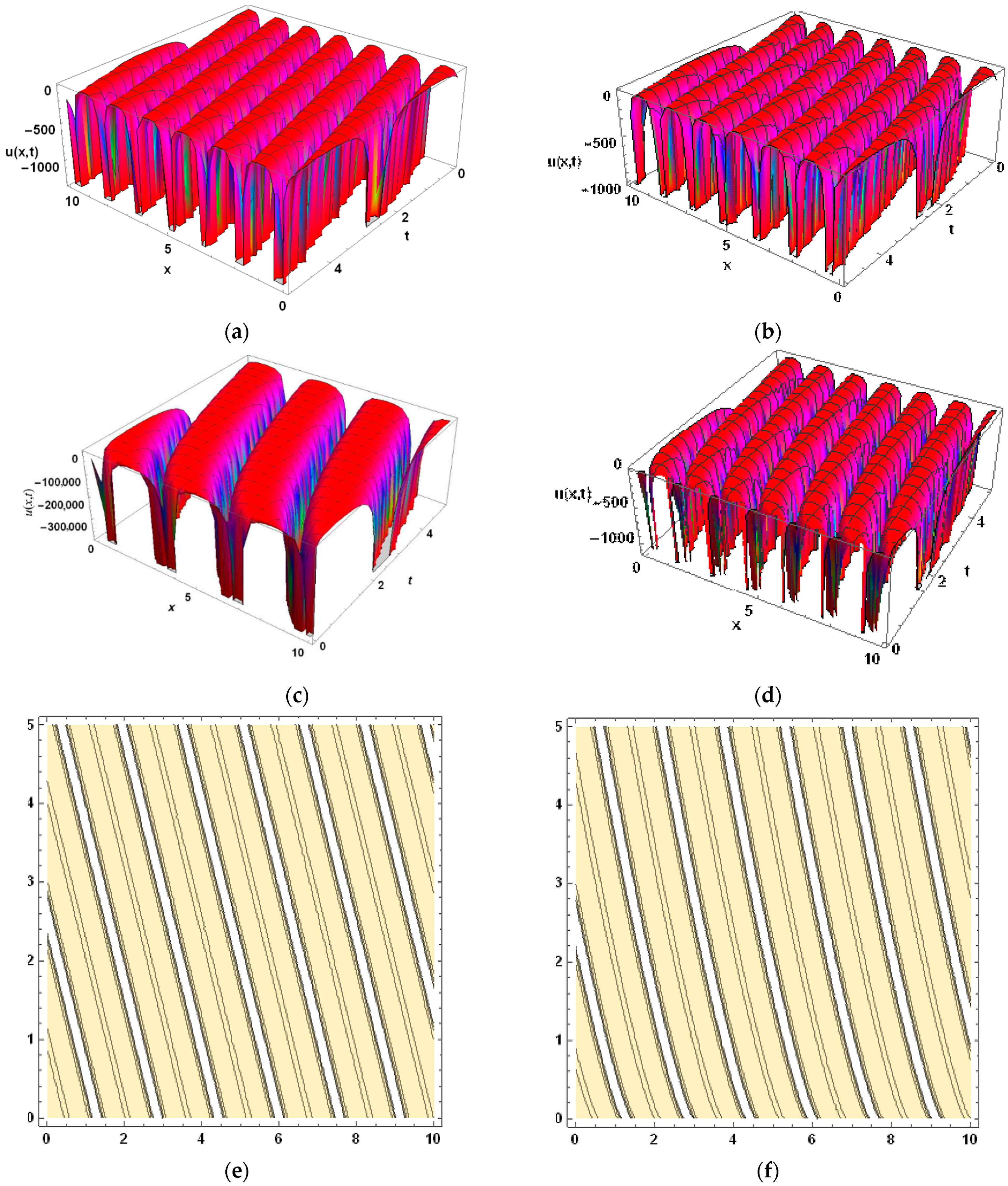
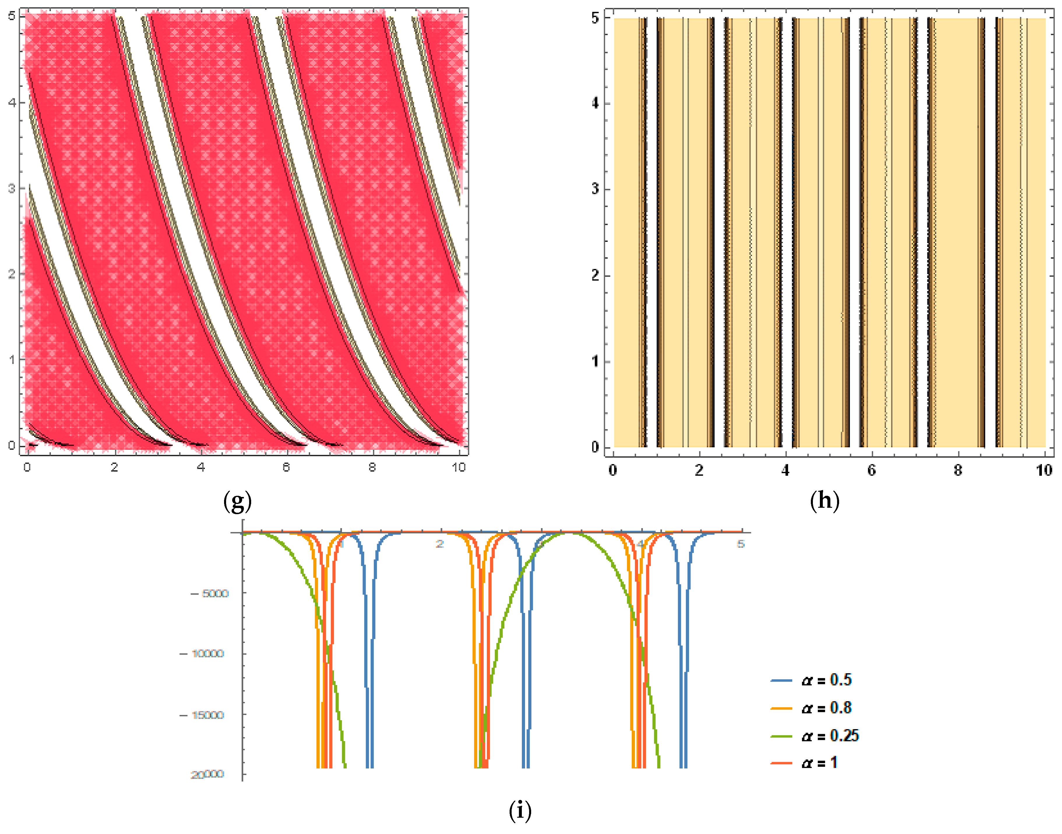
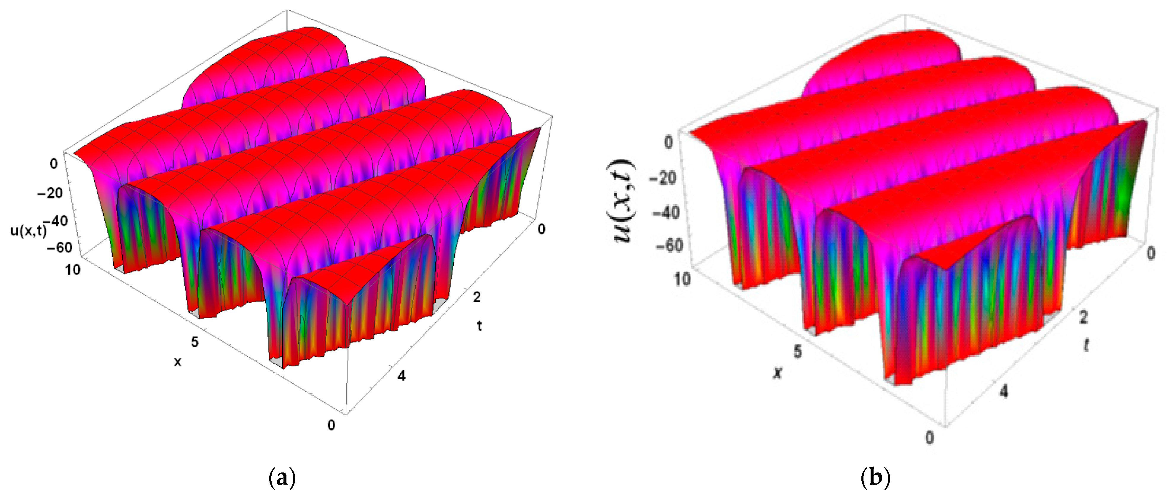
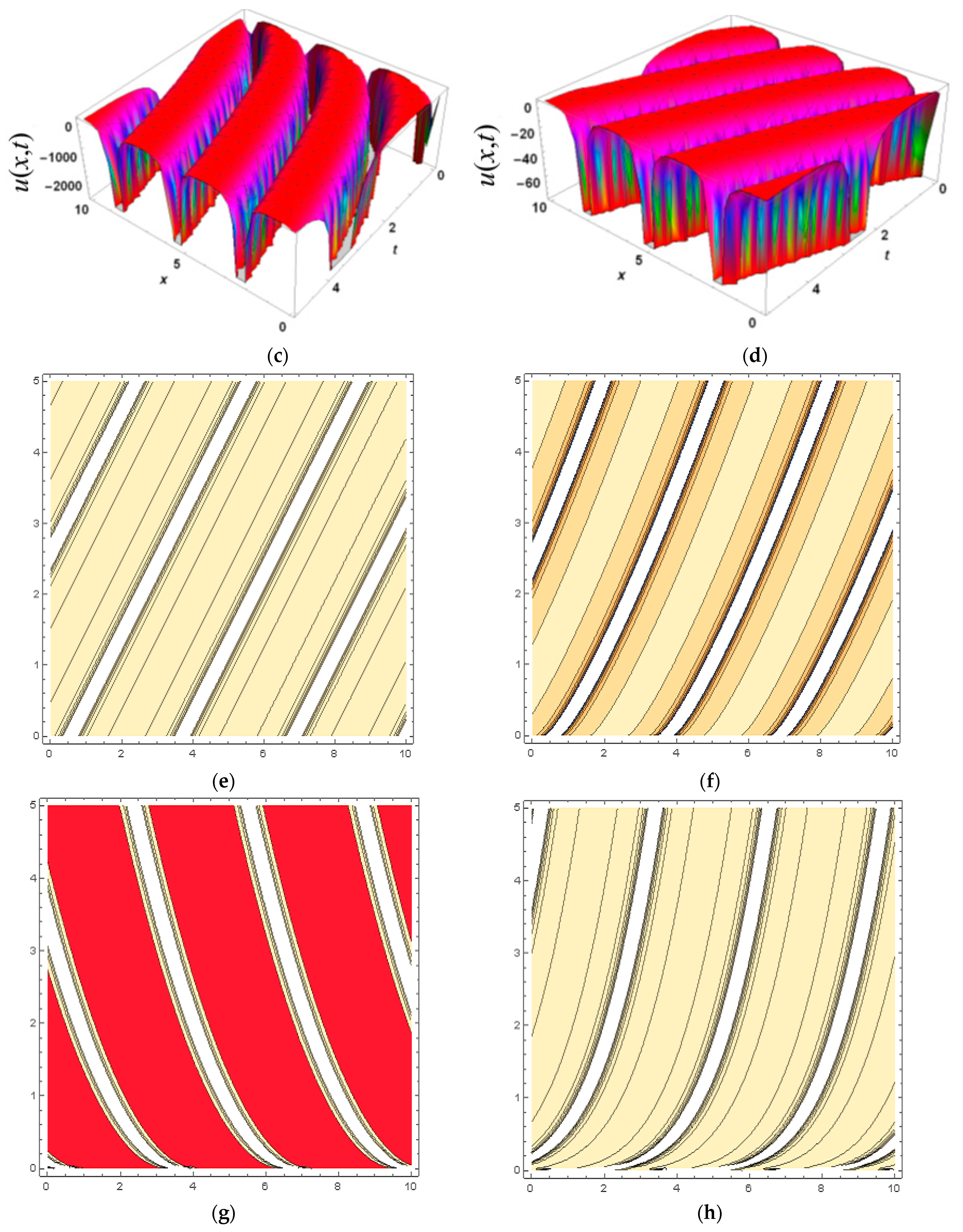
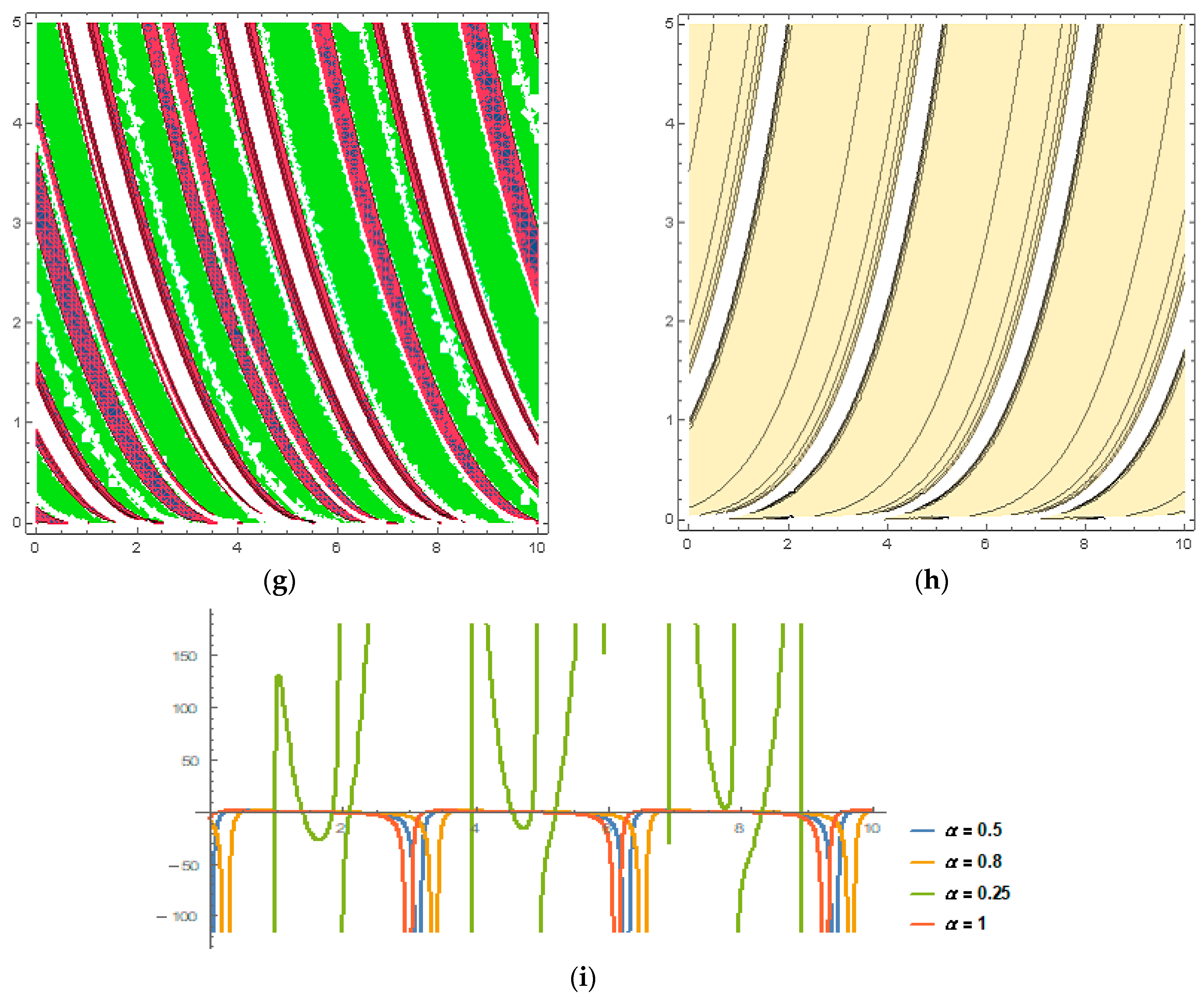
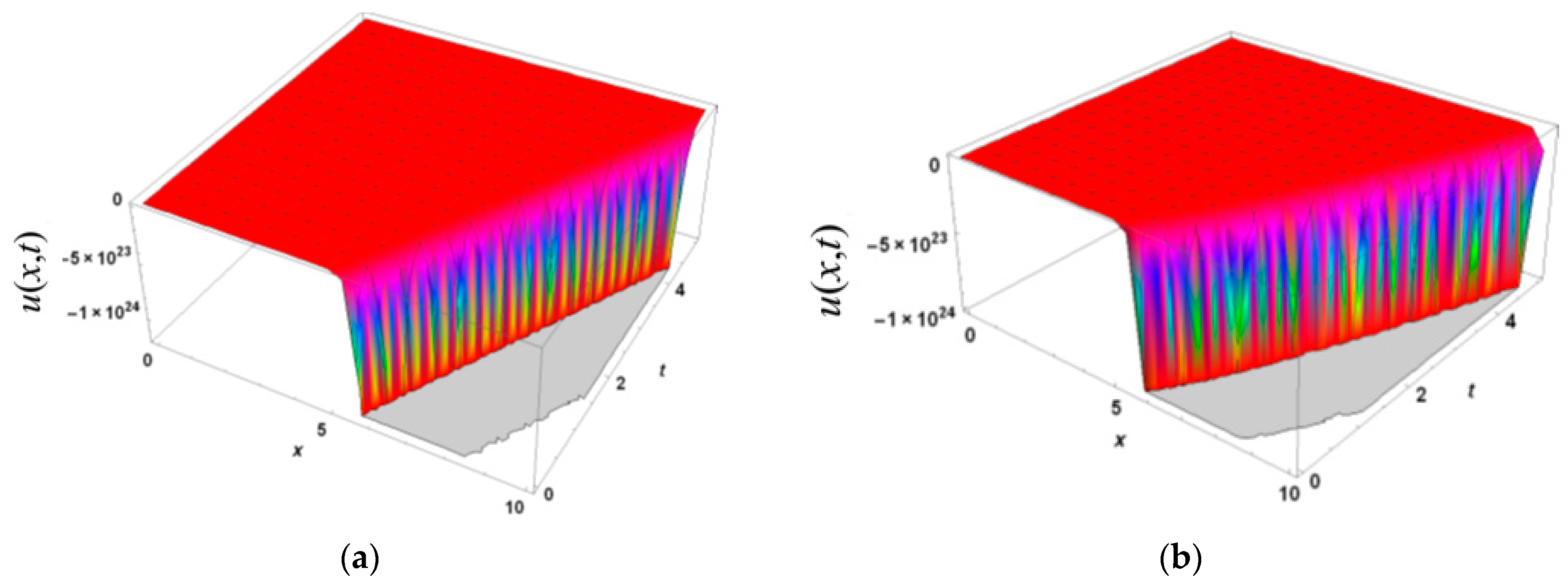
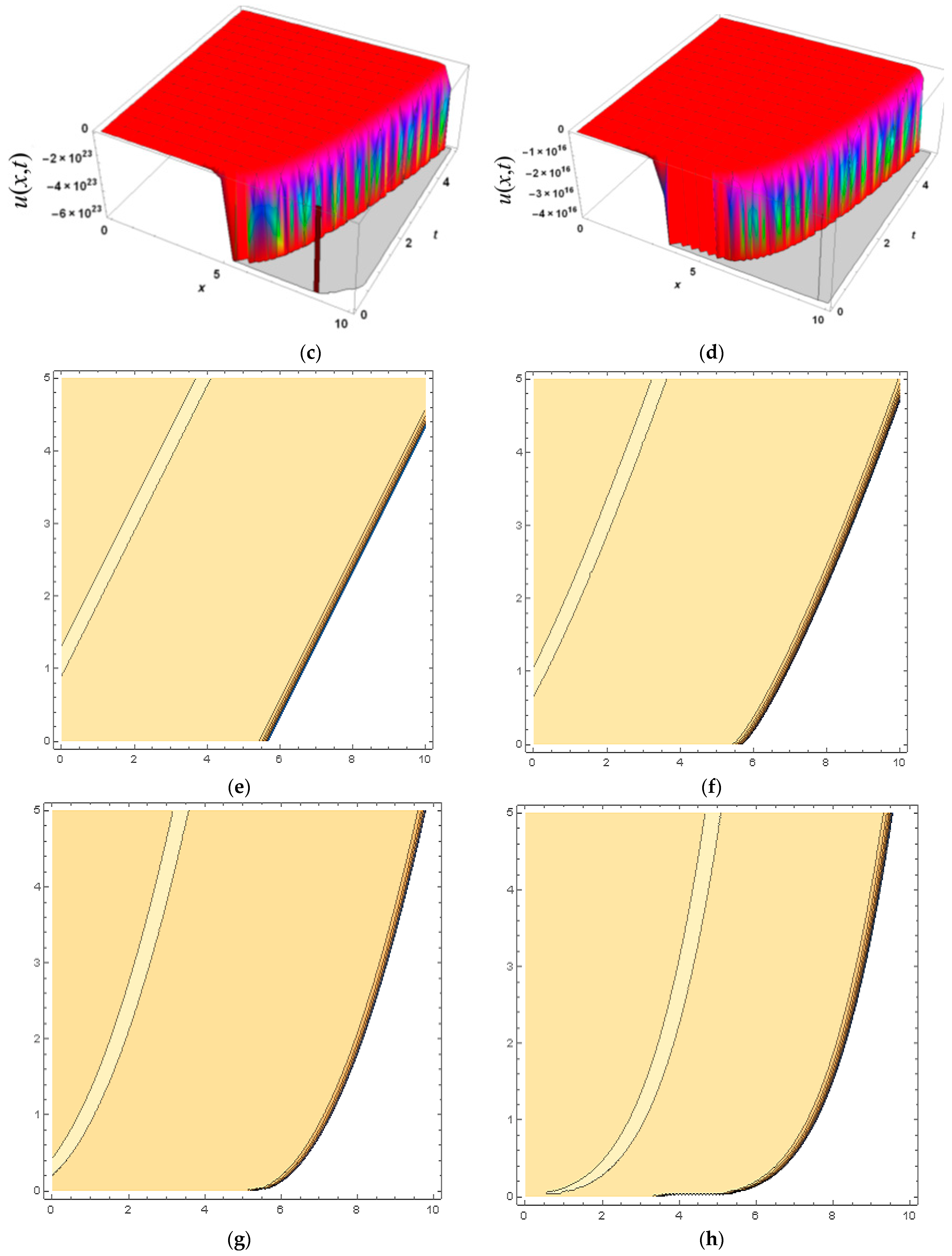
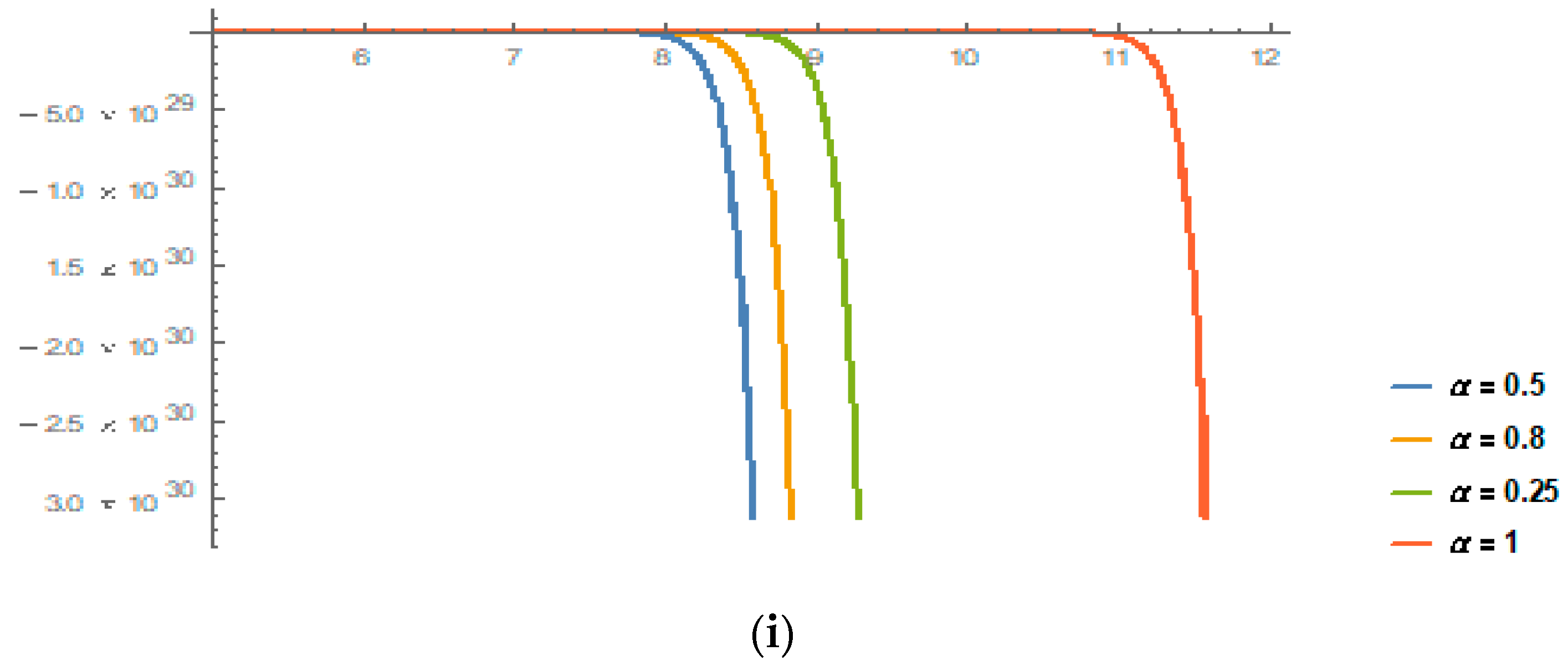
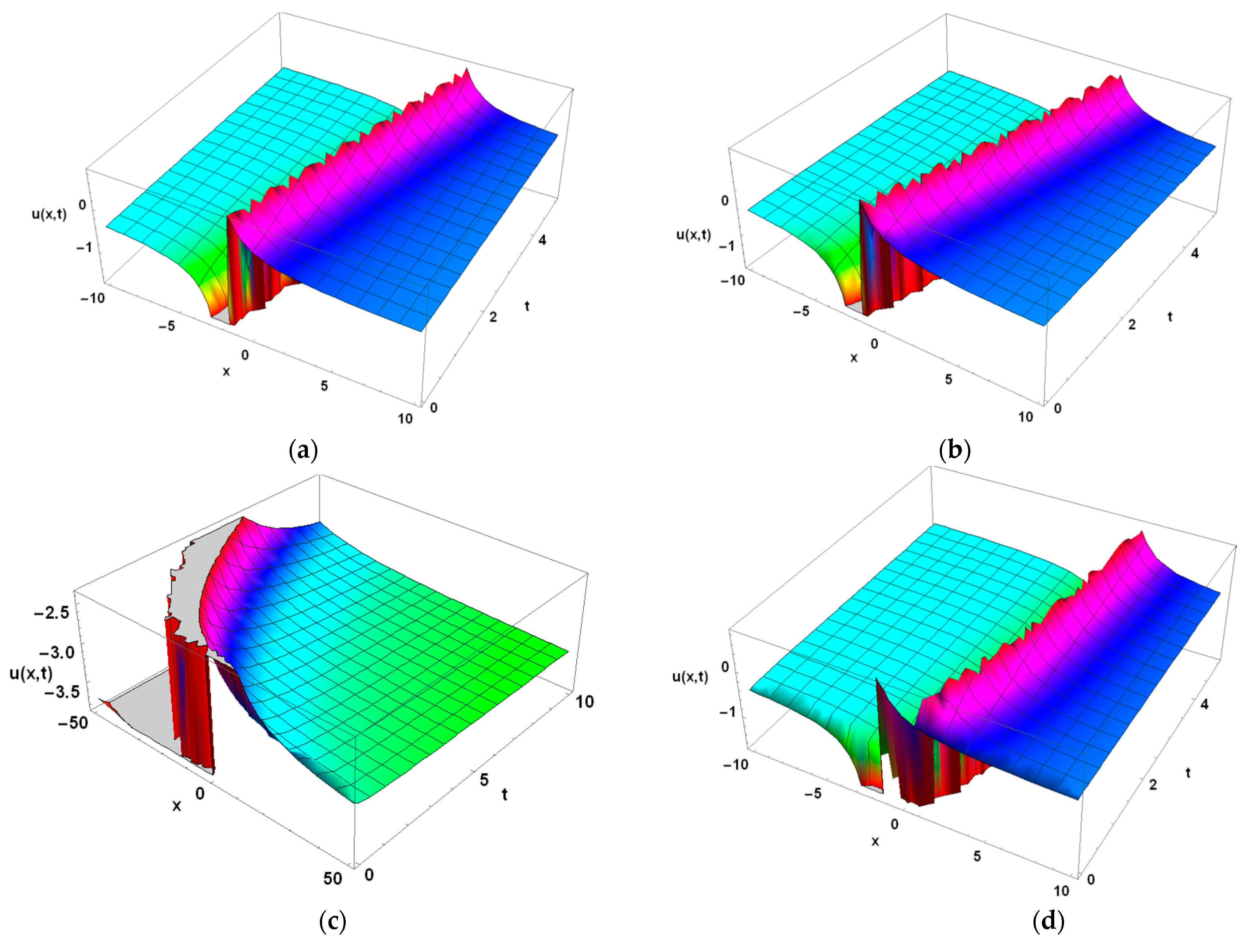
5. Physical Implications and Graphical Analysis

In this paper, the exact analytic results of a fractional-order RWE were extracted by introducing fractional transformation. With the help of numerical simulations, several analytic solutions of RWE were discovered. The outcomes are depicted in the forms of 3D, 2D, and contour profiles. Consequently, the periodic, singular, and anti-singular kink wave solutions were captured for four forms of wave findings that were developed by using this method—these were exponential, rational hyperbolic, and trigonometric functions. The physical phenomena of the results are presented with the help of CAS in Figure 1, Figure 2, Figure 3, Figure 4, Figure 5 and Figure 6, which help us to understand the nature, behavior, properties, and characteristics of the RWE. The behaviors of solitary waves are controlled by assigning different values to the free parameters. Hence, by altering the values of the parameters, the nature of the graph changes. On the other hand, the solution profiles depend on the fractional-order α. For$\alpha =1$, the conformable fractional derivative becomes the classical derivative. Here, we explain how the fractional order affects the graph of the optical solitons found for the fractional nonlinear optics model (RWE) for different sets of variables. For clarification, the figures are shown with respect to $\alpha (0<\alpha \le 1),$which varies with small differences. We discovered two sets of solutions. Set-1 comprises the Equations (21)–(33). Meanwhile, the values of the unknown coefficients produced in set-2 provide different, fresh, and constructive Equations (35)–(46).

The obtained solutions consist of the parameters $A, B,C,c_1,c_2,\beta , \omega ,\mu , k, m,$ and$n$. Figure 1, Figure 2, Figure 3 and Figure 4 present the periodic soliton solutions from Equations (27)–(31) for the values of$A=1, B=4, C=2, c_1=1, c_2=1, \beta =1, \omega =-1, \mu =1, k=1, m=1$, and $n=2.5$. The 3D and contour profiles are represented for$0\le x\le 10$ and $0\le t\le 5$for various values of $\alpha$. The 2D plot is also sketched for $0\le x\le 10 \mathrm{and} t=1$ for various values of $\alpha$.

However, for the values $A=1, B=4, C=2, c_1=1, c_2=1, \beta =1, \omega =-1, \mu =1, k=1, m=1,$ and $n=2.5$ for the variables in Equation (32), we establish a singular soliton solution. In the case of singular solutions, a travelling wave has endless wings on both sides and a nominal space in between them, which causes the wave to be singular. The profile of this figure is widely escalating on one side. The 3D and contour graphs are depicted within the limits$0\le x\le 10$ and $0\le t\le 5$for different values of $\alpha$. The 2D profile is constructed for $0\le x\le 10 \mathrm{and} t=1$(Figure 5).

Again, when $A=1, B=4, C=2, c_1=1, c_2=1, \beta =1, \omega =-1, \mu =1, k=1, m=1,$ and $n=2.5$ for the parameters of Equation (32), we establish the singular and anti-singular kink soliton solutions. The 3D and contour profiles are illustrated within the limits $-10\le x\le 10$ and $0\le t\le 5$. The 2D profile is constructed for $-10\le x\le 10 \mathrm{and} t=1$ (Figure 6).

Figure 1, Figure 2, Figure 3, Figure 4, Figure 5 and Figure 6 demonstrates the fractional-order RWE model with a nonlinear dynamic optical nature for new solitary wave solutions. Applications can be found for these solutions in nonlinear electromagnetic waves, ion- and magneto-soundwaves in plasmas, ocean engineering, and different natural and physical phenomena in science and engineering. Since the graphs of Equations (35)–(46) are similar to those of Equations (21)–(33), we have not presented them in the figures.

In this work, we described different states with several values of free parameters by using fractional derivatives. Fractional derivatives play a crucial role in the understanding of the nature of the proposed problem. In addition to this, a consistent behavior of the traveling wave was demonstrated throughout the article. When it comes to analyzing different kinds of nonlinear fractional evolution equations, these findings illustrate that this is a more reliable, proficient, and dominant technique. Furthermore, different techniques were used on the given model in the literature, but the graphical representations of the acquired results show that the obtained solutions are novel, more contemporary, and more universal than the results that were previously attained.

6. Conclusions

In this article, we used the improved (G’/G)-expansion method to study the fractional-order RWE problem. In comparison with earlier research, the findings of this investigation are being published for the first time. A time-fractional derivative operator was used to analyze the model given above. The main benefit of fractional-order models is that changes gradually develop, and these can be used to graphically illustrate the behavior of the solitary waves in relation to time and space. The graphs of the obtained solutions prove the accuracy and consistency of the above-mentioned method. The accuracy of the results was tested using Maple by plugging the acquired results into the established model. Hence, this method could be used to investigate various nonlinear models that arise frequently in a variety of real-world problems.

References

1. Abdeljabbar, A.; Roshid, H.-O.; Aldurayhim, A. Bright, Dark, and Rogue Wave Soliton Solutions of the Quadratic Nonlinear Klein–Gordon Equation. Symmetry 2022, 14, 1223. [Google Scholar] [CrossRef]
2. Shah, N.A.; Alyousef, H.A.; El-Tantawy, S.A.; Shah, R.; Chung, J.D. Analytical Investigation of Fractional-Order Korteweg–De-Vries-Type Equations under Atangana–Baleanu–Caputo Operator: Modeling Nonlinear Waves in a Plasma and Fluid. Symmetry 2022, 14, 739. [Google Scholar] [CrossRef]
3. Shah, N.A.; Dassios, I.; Chung, J.D. A Decomposition Method for a Fractional-Order Multi-Dimensional Telegraph Equation via the Elzaki Transform. Symmetry 2021, 13, 8. [Google Scholar] [CrossRef]
4. Thach, T.N.; Tuan, N.H. Stochastic pseudo-parabolic equations with fractional derivative and fractional Brownian motion. Stoch. Anal. Appl. 2022, 40, 328–351. [Google Scholar] [CrossRef]
5. Thach, T.N.; Kumar, D.; Luc, N.H.; Tuan, N.H. Existence and regularity results for stochastic fractional pseudo-parabolic equations driven by white noise. Discret. Contin. Dyn. Syst.-S 2022, 15, 481. [Google Scholar] [CrossRef]
6. Shah, N.A.; Agarwal, P.; Chung, J.D.; El-Zahar, E.R.; Hamed, Y.S. Analysis of Optical Solitons for Nonlinear Schrödinger Equation with Detuning Term by Iterative Transform Method. Symmetry 2020, 12, 1850. [Google Scholar] [CrossRef]
7. He, W.; Chen, N.; Dassios, I.; Chung, J.D. Fractional System of Korteweg-De Vries Equations via Elzaki Transform. Mathematics 2021, 9, 673. [Google Scholar] [CrossRef]
8. Nisar, K.S.; Ilhan, O.A.; Abdulazeez, S.T.; Manafian, J.; Mohammed, S.A.; Osman, M. Novel multiple soliton solutions for some nonlinear PDEs via multiple Exp-function method. Results Phys. 2021, 21, 103769. [Google Scholar] [CrossRef]
9. Ma, W.-X. N-soliton solution of a combined pKP–BKP equation. J. Geom. Phys. 2021, 165, 104191. [Google Scholar] [CrossRef]
10. Zhang, S.; Zheng, X. N-soliton solutions and nonlinear dynamics for two generalized Broer–Kaup systems. Nonlinear Dyn. 2022, 107, 1179–1193. [Google Scholar] [CrossRef]
11. Shah, N.A.; Hamed, Y.S.; Abualnaja, K.M.; Chung, J.-D.; Shah, R.; Khan, A. A Comparative Analysis of Fractional-Order Kaup–Kupershmidt Equation within Different Operators. Symmetry 2022, 14, 986. [Google Scholar] [CrossRef]
12. Cinar, M.; Onder, I.; Secer, A.; Yusuf, A.; Sulaiman, T.A.; Bayram, M.; Aydin, H. The analytical solutions of Zoomeron equation via extended rational sin-cos and sinh-cosh methods. Phys. Scr. 2021, 96, 094002. [Google Scholar] [CrossRef]
13. Rani, A.; Zulfiqar, A.; Ahmad, J.; Hassan, Q.M.U. New soliton wave structures of fractional Gilson-Pickering equation using tanh-coth method and their applications. Results Phys. 2021, 29, 104724. [Google Scholar] [CrossRef]
14. Rani, A.; Ashraf, M.; Ahmad, J.; Ul-Hassan, Q.M. Soliton solutions of the Caudrey–Dodd–Gibbon equation using three expansion methods and applications. Opt. Quantum Electron. 2022, 54, 158. [Google Scholar] [CrossRef]
15. Naz, S.; Ul-Hassan, Q.M.; Zulfiqar, A. Dynamics of new optical solutions for nonlinear equations via a novel analytical technique. Opt. Quantum Electron. 2022, 54, 474. [Google Scholar] [CrossRef]
16. Abdel-Salam, E.A.; Gumma, E.A. Analytical solution of nonlinear space–time fractional differential equations using the improved fractional Riccati expansion method. Ain Shams Eng. J. 2015, 6, 613–620. [Google Scholar] [CrossRef] [Green Version]
17. Zayed, E.M.; Alngar, M.E. Optical soliton solutions for the generalized Kudryashov equation of propagation pulse in optical fiber with power nonlinearities by three integration algorithms. Math. Methods Appl. Sci. 2021, 44, 315–324. [Google Scholar] [CrossRef]
18. Mohyud-Din, S.T.; Shakeel, M. Soliton solutions of coupled systems by improved (G′/G)-expansion method. In Proceedings of the AIP Conference Proceedings, Tampa, FL, USA, 9–11 March 2013; pp. 156–166. [Google Scholar]
19. Islam, S.R.; Bashar, M.H.; Muhammad, N. Immeasurable soliton solutions and enhanced (G′/G)-expansion method. Phys. Open 2021, 9, 100086. [Google Scholar] [CrossRef]
20. Rizvi, S.; Seadawy, A.R.; Younis, M.; Ali, I.; Althobaiti, S.; Mahmoud, S.F. Soliton solutions, Painleve analysis and conservation laws for a nonlinear evolution equation. Results Phys. 2021, 23, 103999. [Google Scholar] [CrossRef]
21. Wang, M.; Li, X.; Zhang, J. The (G′ G)-expansion method and travelling wave solutions of nonlinear evolution equations in mathematical physics. Phys. Lett. A 2008, 372, 417–423. [Google Scholar] [CrossRef]
22. Yokus, A.; Durur, H.; Ahmad, H.; Thounthong, P.; Zhang, Y.-F. Construction of exact traveling wave solutions of the Bogoyavlenskii equation by (G′/G, 1/G)-expansion and (1/G′)-expansion techniques. Results Phys. 2020, 19, 103409. [Google Scholar] [CrossRef]
23. Islam, T.; Akbar, M.A.; Azad, A.K. Traveling wave solutions to some nonlinear fractional partial differential equations through the rational (G′/G)-expansion method. J. Ocean Eng. Sci. 2018, 3, 76–81. [Google Scholar] [CrossRef]
24. Mohammed, W.W.; Alesemi, M.; Albosaily, S.; Iqbal, N.; El-Morshedy, M. The Exact Solutions of Stochastic Fractional-Space Kuramoto-Sivashinsky Equation by Using (G′ G)-Expansion Method. Mathematics 2021, 9, 2712. [Google Scholar] [CrossRef]
25. Aniqa, A.; Ahmad, J. Soliton solution of fractional Sharma-Tasso-Olever equation via an efficient (G′/G)-expansion method. Ain Shams Eng. J. 2022, 13, 101528. [Google Scholar] [CrossRef]
26. Younis, M.; Seadawy, A.R.; Baber, M.; Husain, S.; Iqbal, M.; Rizvi, S.; Baleanu, D. Analytical optical soliton solutions of the Schrödinger-Poisson dynamical system. Results Phys. 2021, 27, 104369. [Google Scholar] [CrossRef]
27. Barman, H.K.; Aktar, M.S.; Uddin, M.H.; Akbar, M.A.; Baleanu, D.; Osman, M. Physically significant wave solutions to the Riemann wave equations and the Landau-Ginsburg-Higgs equation. Results Phys. 2004, 22, 683–691. [Google Scholar] [CrossRef]
28. Geng, X.; Cao, C. Explicit solutions of the 2 + 1-dimensional breaking soliton equation. Chaos Solitons Fractals 2004, 22, 683–691. [Google Scholar] [CrossRef]
29. Barman, H.K.; Seadawy, A.R.; Akbar, M.A.; Baleanu, D. Competent closed form soliton solutions to the Riemann wave equation and the Novikov-Veselov equation. Results Phys. 2020, 17, 103131. [Google Scholar] [CrossRef]
30. Hong-Hai, H.; Da-Jun, Z.; Jian-Bing, Z.; Yu-Qin, Y. Rational and periodic solutions for a (2 + 1)-dimensional breaking soliton equation associated with ZS-AKNS hierarchy. Commun. Theor. Phys. 2010, 53, 430. [Google Scholar] [CrossRef]
31. Roy, R.; Barman, H.K.; Islam, M.N.; Akbar, M.A. Bright-dark wave envelopes of nonlinear regularized-long-wave and Riemann wave models in plasma physics. Results Phys. 2021, 30, 104832. [Google Scholar] [CrossRef]
32. Duran, S. Breaking theory of solitary waves for the Riemann wave equation in fluid dynamics. Int. J. Mod. Phys. B 2021, 35, 2150130. [Google Scholar] [CrossRef]
33. Khalil, R.; Al Horani, M.; Yousef, A.; Sababheh, M. A new definition of fractional derivative. J. Comput. Appl. Math. 2014, 264, 65–70. [Google Scholar] [CrossRef]
34. Kajouni, A.; Chafiki, A.; Hilal, K.; Oukessou, M. A New Conformable Fractional Derivative and Applications. Int. J. Differ. Equ. 2021, 2021, 6245435. [Google Scholar] [CrossRef]
35. Abdeljawad, T. On conformable fractional calculus. J. Comput. Appl. Math. 2015, 279, 57–66. [Google Scholar] [CrossRef]
36. Atangana, A.; Baleanu, D.; Alsaedi, A. New properties of conformable derivative. Open Math. 2015, 13, 889–898. [Google Scholar] [CrossRef]
37. Tuan, N.H.; Thach, T.N.; Can, N.H.; O′Regan, D. Regularization of a multidimensional diffusion equation with conformable time derivative and discrete data. Math. Methods Appl. Sci. 2021, 44, 2879–2891. [Google Scholar] [CrossRef]
Figure 1. For Equation (28), (ad) with 0 x 10 , 0 t 5   indicate the 3D profiles, (eh) depict the contour profiles for 0 x 10 and 0 t 5 , and (i) denotes the 2D sketch for various values of α. (a) α = 1 , (b) α = 0.8 , (c) α = 0.5 , (d) α = 0.25 , (e) α = 1 , (f) α = 0.8 , (g) α = 0.5 , and (h) α = 0.25 .
Mathematics 10 04171 g001aMathematics 10 04171 g001b
Figure 2. For Equation (29), (ad) with 0 x 10 and 0 t 5   indicate the 3D profiles, (eh) depict the contour plots for 0 x 10 and 0 t 5 , and (i) indicates the 2D representation of a range of values of α. (a) α = 1 , (b) α = 0.8 , (c) α = 0.5 , (d) α = 0.25 , (e) α = 1 , (f) α = 0.8 , (g) α = 0.5 , and (h) α = 0.25 .
Mathematics 10 04171 g002aMathematics 10 04171 g002bMathematics 10 04171 g002c
Figure 3. For Equation (30), (ad)with 0 x 10 and 0 t 5   denote the 3D profiles, (eh) express the contour profiles for 0 x 10 and 0 t 5 , and (i) indicates the 2D representation of a range of values of α. (a) α = 1 , (b) α = 0.8 , (c) α = 0.5 , (d) α = 0.25 , (e) α = 1 , (f) α = 0.8 , (g) α = 0.5 , and (h) α = 0.25 .
Mathematics 10 04171 g003aMathematics 10 04171 g003b
Figure 4. For Equation (31), (ad) with 0 x 10 and 0 t 5   express the 3D profiles, (eh) show the contour profiles for 0 x 10 and 0 t 5 , and (i) indicates the 2D representation of a range of values of α. (a) α = 1 , (b) α = 0.8 , (c) α = 0.5 , (d) α = 0.25 , (e) α = 1 , (f) α = 0.8 , (g) α = 0.5 , and (h) α = 0.25 .
Mathematics 10 04171 g004aMathematics 10 04171 g004b
Figure 5. For Equation (32), (ad) with 0 x 10 and 0 t 5   indicate the 3D profiles, (eh) represent the contour profiles for 0 x 10 and 0 t 5 , and (i) indicates the 2D representation of a range of values of α. (a) α = 1 , (b) α = 0.8 , (c) α = 0.5 , (d) α = 0.25 , (e) α = 1 , (f) α = 0.8 , (g) α = 0.5 , and (h) α = 0.25 .
Mathematics 10 04171 g005aMathematics 10 04171 g005bMathematics 10 04171 g005c
Figure 6. For Equation (33), (ad) with 10 x 10 and 0 t 5   indicate the 3D profiles, (eh) express the contour profiles for 10 x 10 and 0 t 5 , and (i) indicates the 2D representation of a range of values of α. (a) α = 1 , (b) α = 0.8 , (c) α = 0.5 , (d) α = 0.25 , (e) α = 1 , (f) α = 0.8 , (g) α = 0.5 , and (h) α = 0.25 .
Mathematics 10 04171 g006aMathematics 10 04171 g006b