Article

Modeling for the Relationship between Monetary Policy and GDP in the USA Using Statistical Methods

by
Andre Amaral
1,
Taysir E. Dyhoum
1,2,3,*,
Hussein A. Abdou
4,5 and
Hassan M. Aljohani
6,*
1
School of Computing, Faculty of Science, Technology, Engineering and Mathematics, Arden University, Coventry CV3 4FJ, UK
2
School of the Natural Sciences, Faculty of Science and Technology, University of Central Lancashire, Preston PR1 2HE, UK
3
Department of Mathematics & Statistics, Faculty of Science, Misurata University, Misurata 21851, Libya
4
School of Business, Faculty of Business & Justice, University of Central Lancashire, Preston PR1 2HE, UK
5
Department of Management, Faculty of Commerce, Mansoura University, Mansoura 35511, Egypt
6
Department of Mathematics & Statistics, College of Science, Taif University, P.O. Box 11099, Taif 21944, Saudi Arabia
*
Authors to whom correspondence should be addressed.
Mathematics 2022, 10(21), 4137; https://doi.org/10.3390/math10214137
Submission received: 24 August 2022 / Revised: 20 October 2022 / Accepted: 21 October 2022 / Published: 5 November 2022
(This article belongs to the Special Issue Probability, Statistics and Their Applications 2021)

Abstract

:
The Federal Reserve has played an arguably important role in financial crises in the United States since its creation in 1913 through monetary policy tools. Thus, this paper aims to analyze the impact of monetary policy on the United States’ economic growth in the short and long run, measured by Gross Domestic Product (GDP). The Vector Autoregressive (VAR) method explores the relationship among the variables, and the Granger causality test assesses the predictability of the variables. Moreover, the Impulse Response Function (IRF) examines the behavior of one variable after a change in another, utilizing the time-series dataset from the first quarter of 1959 to the second quarter of 2022. This work demonstrates that expansionary monetary policy does have a positive impact on economic growth in the short term though it does not last long. However, in the long term, inflation, measured by the Consumer Price Index (CPI), is affected by expansionary monetary policy. Therefore, if the Federal Reserve wants to cease the expansionary monetary policy in the short run, this should be done appropriately, with the fiscal surplus, to preserve its credibility and trust in the US dollar as a global store of value asset. Also, the paper’s findings suggest that continuous expansion of the Money Supply will lead to a long-term inflationary problem. The purpose of this research is to bring the spotlight to the side effects of expansionary monetary policy on the US economy, but also allow other researchers to test this model in different economies with different dynamics.

1. Introduction

1.1. Research Background

Monetary policy controls the economy’s total Money Supply, composed of M1 and M2. M1 is the total money held by the public and used for deposits, checking accounts, transactions, and payments, which can be the currency, checks, and negotiable order of withdrawal (NOW) accounts. While M2 also consists of M1 components plus assets with high liquidity (Liquidity refers to assets that can be converted easily into cash in a short period; this is considered to be one fiscal year [1]). There is no consensus about the origin of money, but there is a comprehensive agreement that many different objects are used to exchange goods, stores of value, and units of account, such as gold and silver.
Central Banks across the world, in general, have different monetary policies and tools to apply. There are two popular types of monetary policy, they are expansionary and contractionary. The first tool of monetary policy is called the open market (OMO). This type is when the FED wants to add more liquidity to the economy, which is done by buying treasury bonds from commercial banks, increasing their reserves, and allowing them to lend more. This move is what is known as expansionary monetary policy. In the long run, the actual effect of open market operations is questionable, as [2,3] found. The opposite is also true; when the FED sells treasury bonds, banks lend less due to liquidity shortages in the economy. This is how the government can raise funds for its investments and expenses. Open Market transactions help to set the funds rate, which will determine the national interest rate. Additional monetary policy tools are used by the FED, such as Reserve requirements and the discount rate. The discount rate is a type of interest charged by the FED on credit facilities provided by the central bank to ensure that depository institutions meet their reserve requirement threshold.

1.2. Relevant Theoretical and Empirical Reviews

In this part of the introduction, we discuss the theoretical and empirical literature reviews that provide a clear idea of what other researchers have done and their outcomes and critically reflect on a potential grasp of up-to-date published information on the topic. This part presents a solid foundation for this paper, it identifies the research gaps presented and cites the up-to-date/latest reviews of the literature that is relevant to this research.
The increase in Money Supply to enhance GDP has long been an object of discussion among economists. For some of them, when interest rates are close to zero, an increase in Money Supply will not be effective. This is called a liquidity trap, and it was first discovered by [4,5] and was recently discussed in [6,7,8,9]. In such a case, under economic crises, agents prefer liquidity over debt; in other words, firms and households would prefer holding cash instead of acquiring credit for investments or consumption. The long-run economic goals of the American Federal Reserve and Federal Open Market Committees are to improve monetary policies and strategies to achieve reasonable stability in goods prices and lower the inflation rate, maximize employment, and tackle the challenges of monetary policy constituted by a continuously low-interest rate [10,11,12].
Financial and economic modeling can help value businesses decide whether to raise capital, expand organically, or buy other shares. In recent work by [13], the economic growth phenomenon was modeled and studied in seven countries over the period from 1990 to 2019. Batrancea and other researchers in [14,15] also recently investigated and analyzed the impact of fiscal pressure on the financial short-term and long-term equilibrium of energy (gas and electricity) companies listed on the New York Stock Exchange over 16 years. Batrancea [16] modeled and examined the impact of the financial liquidity and financial solvency that influenced the performance of 34 healthcare companies. This research work aims to empirically test the efficiency of monetary policy developed by the American central bank Federal Reserve (FED), to foment economic growth in the United States. It also answers the question of ‘How much benefit does expansionary monetary policy brings to economic growth?’ To examine the significance of monetary policy on Gross Domestic Product (GDP) growth, we will perform the Vector Autoregressive (VAR) model, Granger causality test, and Impulse Response Function (IRF). We will analyze the hypothesis to determine whether the expansionary monetary policy creates economic growth. It is interesting to see how Kamaan [17] used the VAR methodology to find that a one-standard-deviation monetary policy shock has a negative and insignificant effect on output. Bernake and Blinder [18] found that contractionary monetary policy or ‘tight money’ reduces the volume of deposits held by depositary institutions. In addition, they also noted that loans tend to fall shortly after the fund’s rates move while financial institutions’ balance sheets are adjusted. Given the contractionary monetary policy, the fall in deposits fully establishes the reduction of loans after two years.
The classical theory of money [19] gained a new approach from Friedman [20], who stated that his theory is, in the first place, a theory of the demand for money and not a theory of output, money income, or price level. Therefore, any increase in real income increases the need for money (DM), which he described as any other asset. Thus, DM or M P can be understood as a function of total wealth, the division of wealth between humans and non-humans, the expected rate of return of other assets, and preferences of wealth holders; mathematically, this is:
M P = f w ,   r t   ,   r a   ,   1 P . d P d t ,   y ,   u
where:
  • M   = money balance desired by the public;
  • P   = price level;
  • y = total wealth;
  • w = relation between human wealth and non-human;
  • r t = expected rate of return over bonds;
  • r a = expected rate of return overstocks;
  • u = taste and preference.
By arranging the above equation as like the classical Quantity Theory of Money:
    M = 1 v P y ,
If k = 1 / v , then:
      M = k P y
where k represents the ratio of the desired money held by the public as a constant. Therefore, an increase in Money Supply by the Federal Reserve bonds purchase scheme would affect those holders who sell. This increases their money balance that will be spent on assets, goods, and services, increasing nominal income (Nominal income is before inflation deduction or adjustment called real income). The opposite is also true; if the Federal Reserve (FED) sells bonds, it will reduce the holders’ money balance, reducing goods and services purchases and reducing nominal income. Hence, either way, the demand for money remains constant.
Nevertheless, monetary policy nowadays continues to be the object of analysis by different researchers and methodologies. Kamaan [17] analyzed monetary policy in the developing economy of Kenya; the methodology used was vector autoregression (VAR), a linear equation model where each variable is explained by its own lagged value plus the current values of the remaining variables. This structure is suitable for capturing the dynamics of time series data, and it is straightforward to interpret its output. Besides, VAR is commonly used for multivariate time series analysis. Those variables were gross domestic product, consumer price index, credit to the private sector, central bank rate, treasury bills, lending rate, and nominal effective exchange rate as endogenous (An endogenous variable, in econometrics, refers to a variable determined within the model being analyzed). The study found that GDP growth is not impacted by monetary policy shocks, suggesting that there are other factors and, thus, different alternatives to positively impact total GDP; however, interest rates and credit channels seem more effective for this purpose. In addition, the author concludes that an increase does not follow an unexpected rise in the Central Bank of Kenya’s output rate. A different approach to test the effectiveness of the central bank’s policy to control the interest in inflation and Unemployment Rates in Romania and the European Union was taken in [21]. The result shows a significant relationship between the interest rate and inflation, which allows the central bank to curb inflation when it spikes. An inverse relationship was also found between inflation and the Unemployment Rate, and thus, by controlling inflation, the central bank can prevent an increase in the unemployment rate [21]. Bhattarai [22], in his analysis, verified that there is a relationship between inflation and unemployment among the Organisation for Economic Co-operation and Development (OECD) countries in the long run.
The datasets analyzed are quarterly data series of all OECD members’ inflation, Unemployment Rate, and growth rate from January 1991 to April 2014. The methodologies applied were a correlation, cointegrations, and causality tests. Moreover, the relationship between the growth and employment rates will be tested through Okun’s law or (Okun’s curve) along with linear regression and VAR (The Okun’s law curve was a report by Arthur Okun in 1962 that shows a damaging regularity of a short-run relationship between unemployment and output [23]). As a result, the Phillips curve correlation test was significant for 28 out of 37 countries, including the United States (Phillips [24] tested the rate of change of money wage rates in the United Kingdom, explained by the level of unemployment and the rate of change of unemployment). Hence, it identified that the Phillips curve, or the trade-off between inflation and unemployment, was more significant in developed economies such as Australia, Denmark, France, Italy, the Netherlands, Spain, New Zealand, the UK, and the US. However, no evidence was found for countries like Austria, Germany, and Norway. Islam et al. [25] traced the relationship patterns between monetary policy and economic growth in Bangladesh and the UK, and studied the long-run and short-run impact of monetary policy on economic growth. This study covered the period from 1980 to 2019. The author used the vector error correction model (VECM), which is more desirable when the dataset is non-stationary. Bhara and Malliaris [26] modeled the US monetary policy using a new quantitative approach and the Markov shifting econometric model. They aimed to learn lessons on how to reduce the high unemployment due to the COVID-19 financial crisis. In that study, they rely on a monthly dataset from 2002 to 2015. Feldkircher et al. [27] also conducted a study that measured the effectiveness of American monetary policy during the COVID-19 recession using a new mixed frequency vector autoregressive (MF-VAR) model. The sample period was from the 1st of 2011 to the 24th week of 2020. Furthermore, other recent pieces of research examined the effects of monetary policy on the GDP during the pre-zero lower bound (pre-ZLB), ZLB, or post-ZLB periods. For example, the Federal Reserve applying unconventional monetary policy and lowering the federal funds rate to nearly zero [6,28,29].
Therefore, this paper captures the evolution of the Money Supply in the United States concerning GDP, Interest Rates, Inflation Rate, and Unemployment Rate over a more inclusive period using a Vector Autoregression model (VAR) after ensuring that all model variables are stationaries. Hence, VAR becomes the best fit model. The rest of the paper is organized as follows: Section 2 is the methodology applied thoroughly explained, theoretically and mathematically. Section 3 contains the tests conducted with the obtained results to be exposed and interpreted, and Section 4 is the conclusion. Thus, this paper aims to provide evidence for the real impact of monetary policy on economic growth and inflation in the short and long run.

2. Methodology

In this paper, the VAR model is developed and analyzed to measure the relationship between GDP, Money Supply (M2), Consumer Price Index (CPI), Interest rate (IR), and Unemployment Rate (Unemp), and their past values with no assumptions made. The Granger causality test analyzed if a one-time series Granger causes the other or whether a time series can be used to predict the others. Moreover, the impulse response function (IRF) measures the reaction of one variable to a shock in the other. It is a valuable tool to examine the response of gross domestic product to a variation in Money Supply and Interest Rate. This study explores the time series dataset composed of five macroeconomics aggregates from the first quarter of 1959 to the second quarter of 2022 collected from the Federal Reserve’s website (https://fred.stlouisfed.org) https://fred.stlouisfed.org/series/M2SL (accessed on 15 June 2022).
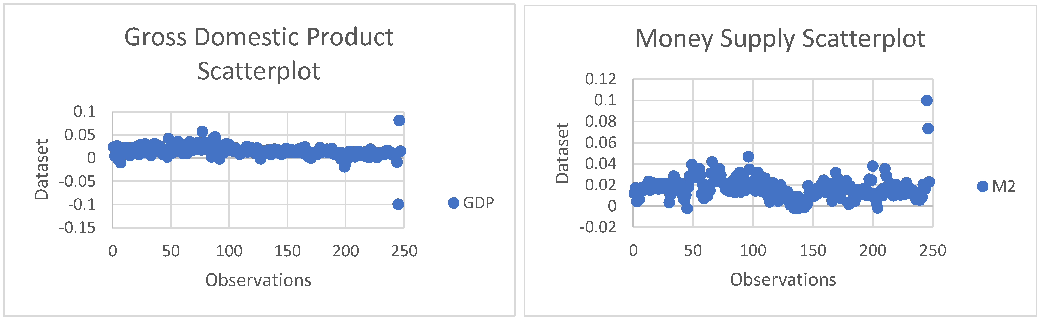
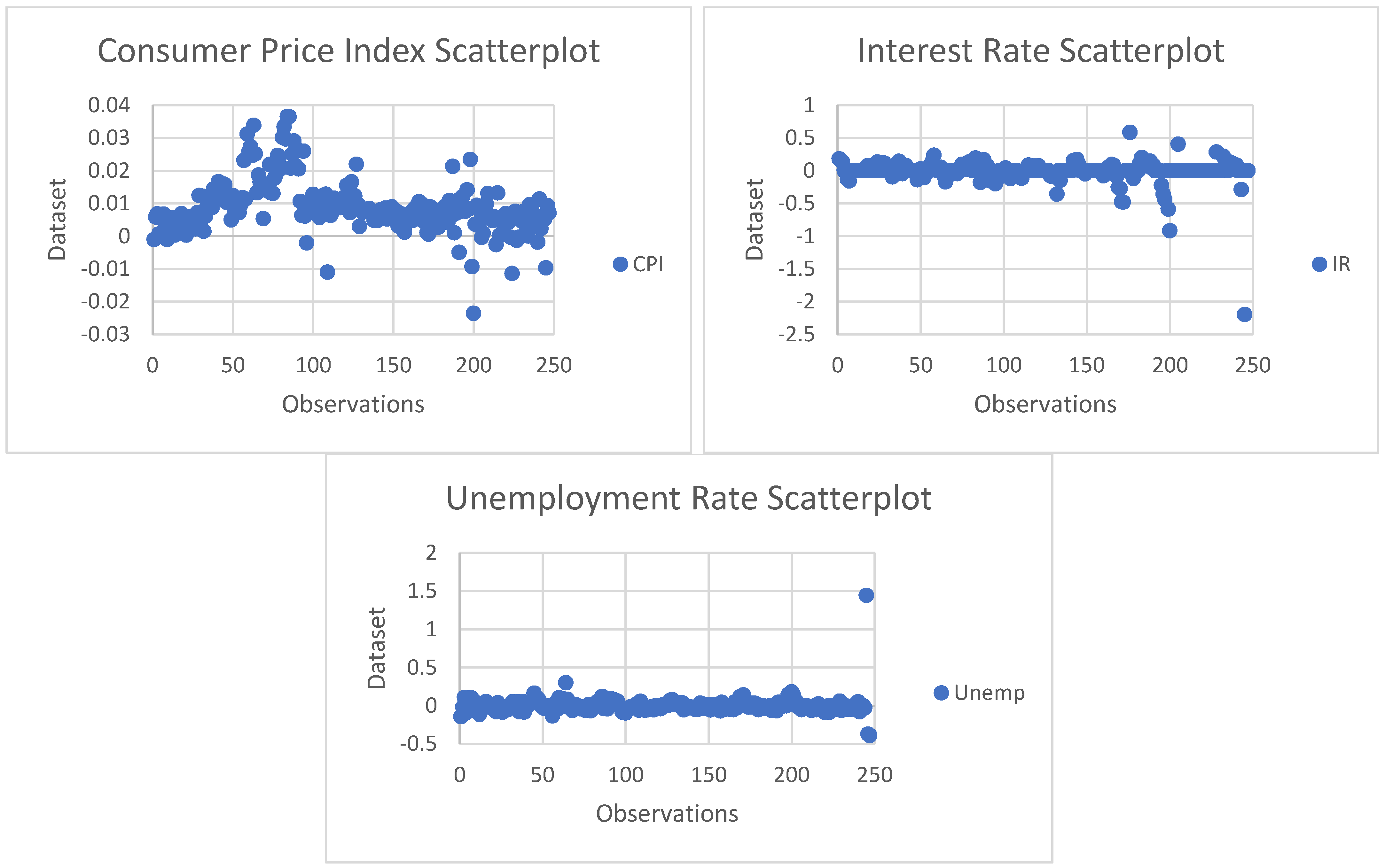
The software utilized in these analyses were R and Microsoft Excel. The dataset comprises 254 observations; however, it is worth stating that the last observation is sacrificed due to the normalization techniques applied and four used as lagged values of the VAR model, which leaves the total sample with 250 observations. Furthermore, the range calculation indicates high variability in the dataset, which can also be confirmed by the large standard deviation in the cases of GDP, M2, and CPI. That is, the data is more spread out around the mean; however, as for Interest Rate and the Unemployment Rate, there is less variability, and the data is more clustered around its mean. In addition, it is pivotal to state that the data does not suffer from skewness or kurtosis as the acceptable range for skewness is ±2, and for kurtosis ±3, according to [30].
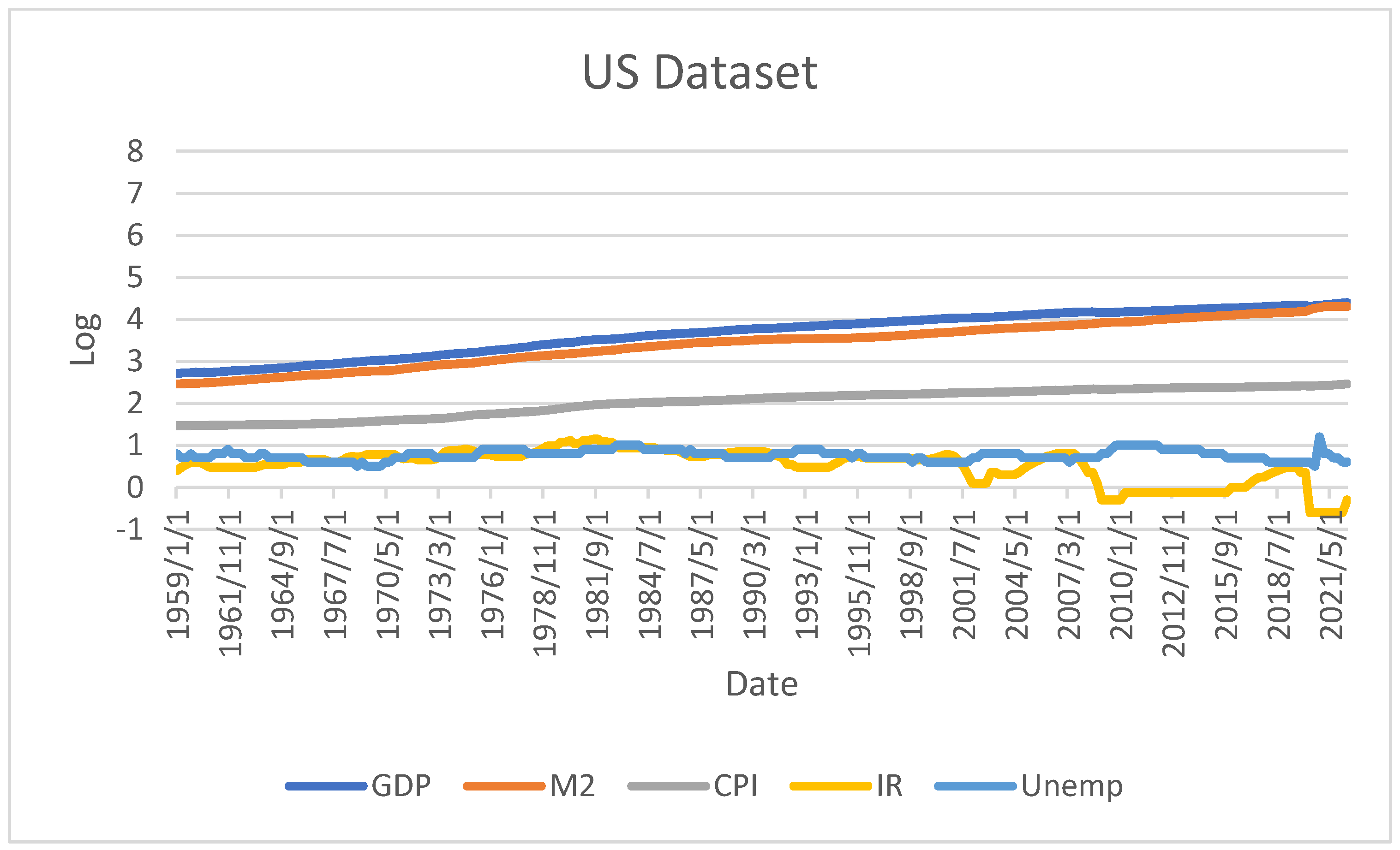
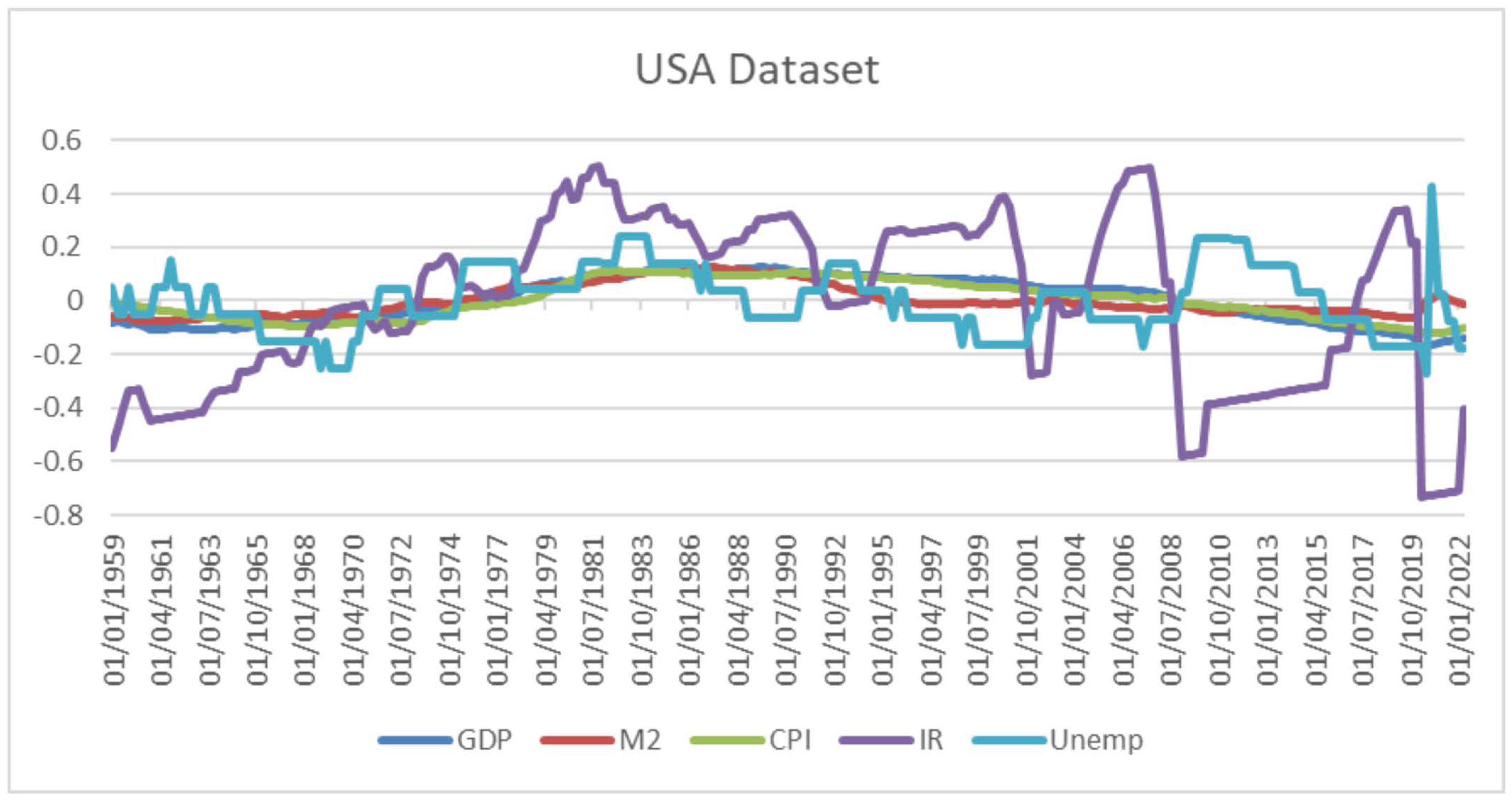
These variables have been extensively explored over the years, and with different research approaches, many theories have evolved. Among those is the relationship between expansionary monetary policy and GDP growth. When working with a macroeconomic dataset, it is common to come across non-stationary data (A dataset is considered stationary when its mean and variance are constant over time [31]), especially when the analysis involves variables such as Growth Domestic Product (GDP), Money Supply (M2), and Consumer Price Index (CPI). Because these variables are not volatile, they usually have an upward or downward trend in an extensive dataset, which must be corrected before any econometric analysis to avoid spurious output and, therefore, misleading interpretation. Hence, the solution to transform non-stationary data to stationary is to take the log of the variables to normalize them and then apply a lagged differencing methodology:
Δ ln Y = ln Y t   ln Y t n
Δ ln X = ln X t   ln X t n
The basic econometric models are separated into two or more variables, a dependent variable called Y t and one independent variable called X t . Thus, the model tests the capability of X t to affect Y t but not the opposite; therefore, in this model, X t is classified as exogenous while Y t is endogenous.

Vector Autoregressive (VAR) Model

The paper has been constructed based on the Vector Autoregressive (VAR) model that [32] advocated as an alternative for regular econometric models that consist of the assumption of X causing Y . Therefore, VAR is a theory-free method that allows the dataset to speak for itself with no prior assumptions made. The model proposed by VAR is a regression model for multivariate time series data when there is more than one dependent variable since all variables within the model can affect each other. In such a case, there might be a mutual relationship between all variables in the model, taking into account a lagged period, which can be any. So, all variables are considered endogenous. Hence, if we convert this into a mathematical equation, then we have (6) and (7), as similarly observed in [31,33,34].
Y t = β 10     β 12 X t   +   ϒ 11 Y t 1 + ϒ 12 X t 1   +   µ yt
X t = β 20 β 21 Y t + ϒ 21 Y t 1 + ϒ 22 X t 1 + µ xt
The VAR model, however, works based on two assumptions:
  • Y t and X t are stationary, also known as A(0), and there is a constant mean and variance over time (t);
  • The error terms µ y t and µ x t are not correlated since it is random.
The issue with the equation above is that the Y t and X t equations are separate. The objective is to have an interrelation between both equations. This is why all endogenous variables are kept to the left side of the equation, whilst the exogenous variables are kept to the right. The solution for this is to algebraically transform the equations into a reduced form, as observed in Equations (8) and (9) below:
Y t β 12 X t   =   β 10 + ϒ 11 Y t 1 + ϒ 12 X t 1 +   µ yt
β 21 Y t + X t = β 20 + ϒ 21 Y t 1 + ϒ 22 X t 1 + µ xt
Once the equations are aligned, we can convert them into a matrix:
1 β 12 β 21 1 Y t X t = β 10 β 21 + ϒ 11 ϒ 12 ϒ 21 ϒ 22 Y t 1 X t 1 + µ yt µ xt
We can simplify the matrices as follows:
β × Φ t = λ   +   δ   × Φ t 1 +   µ t
β Φ t =   λ   +   δ Φ t 1 +   µ t
where:
  • β = 1 β 12 β 21 1 ;
  • λ = β 10   β 21 t ;
  • δ = ϒ 11 ϒ 12 ϒ 21 ϒ 22 ;
  • Φ t = Y t   X t t ;
  • Φ t 1   = Y t 1   X t 1 t ;
  • µ   = µ yt   µ xt t .
We then have β representing the β 12 and β 21 , Φt representing the vector of variables ( Y t ), λ1 the constant, Φ t 1 is the lagged variable, and µ t as the error term. Because β 1 is supposed to be on the right side of the equation, we then multiply both sides of the equation by the inverse matrix of β 1 , and we get:
β 1   Φ t   =   β 1 λ +   β 1 δ   + Φ t 1 +   β 1 +   β 1 µ t
Thus, we finally obtain the reduced form of the equation, and we can simplify once more by renaming the terms:
  I   Φ t = 1 + Φ t 1 + e t  
where:
Ι is the unit matrix and β 1 λ is a constant as β 1 and λ are constants matrices defined as Ω1. We can simplify Equation (14) as:
Φ t = 1 +   Φ t 1   + e t
where:
  • Φ t = Y t X t t ;
  • Φ t 1 = Y t 1   X t 1 t ;
  • e t = µ yt µ xt t .
The VAR model explained above assumes two endogenous variables, X and Y , that are now Φ t 1 but there is no limit to that, and the more variables added, more equations are expected. It is also important to note that in this VAR model Ordinary Least Squares (OLS) will be used to estimate the coefficients of the matrices as similarly done by Feldstein and Stock [
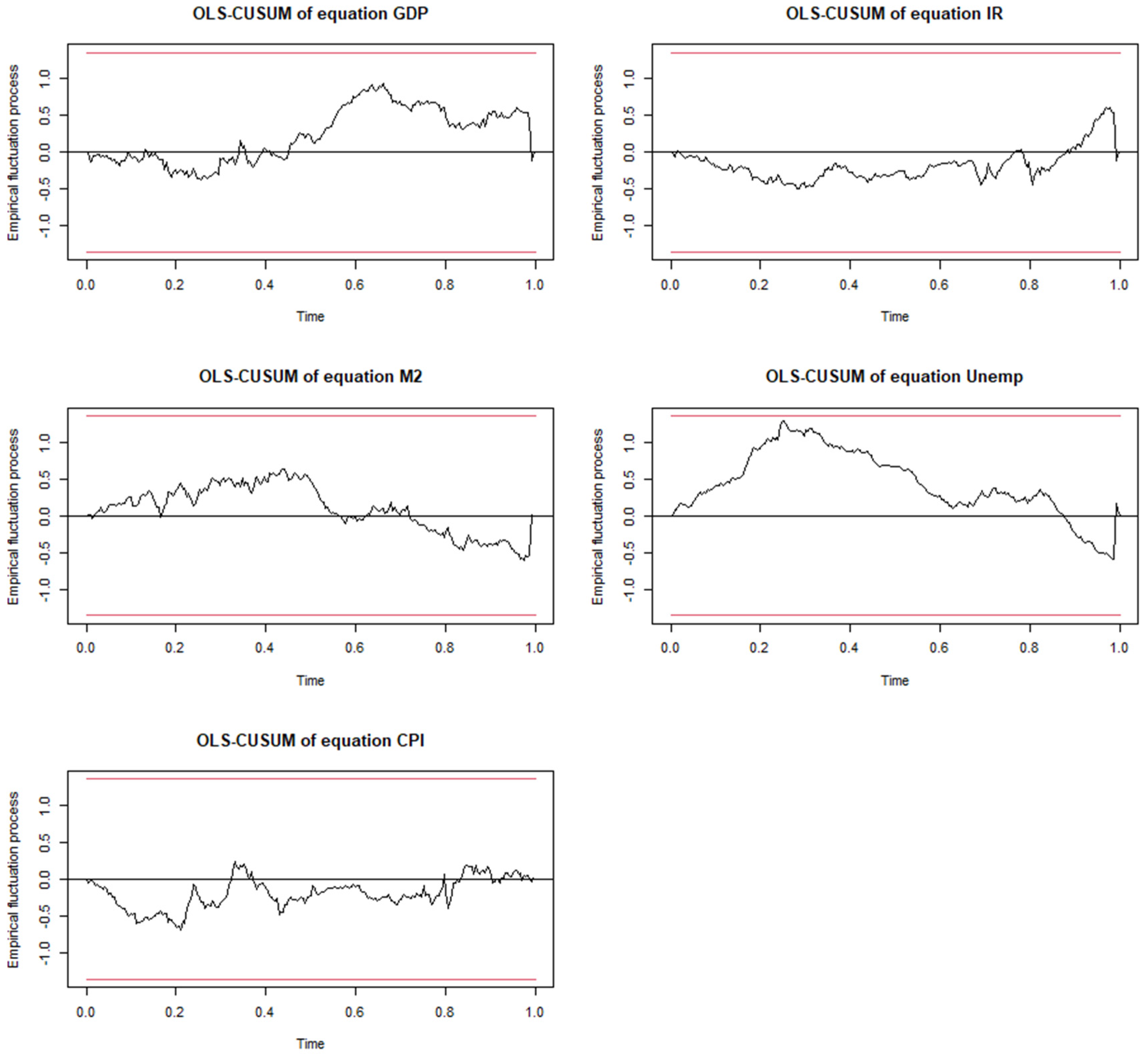
4]. Moreover, it is pivotal to test the VAR model stability, which is done by identifying the root of the Ω matrix. Thus, if the root is less than 1 in absolute value then the system is stable. What is interesting to note is that in case of violation of assumptions 1 and 2, the model would provide a spurious but convincing output, e.g., a high coefficient of determination (R2) as well as statistically significant values (The coefficient of determination, also known as R squared (R2), measures, in percentage, the variability of the dependent variable in relation to changes in the independent variable). Therefore, to avoid this before applying the model, the researcher must perform a stationarity test. In this case, the model is the unit root test (The unit root test is used to determine whether a time series is stationary. A dataset is considered stationary if changes in the variable do not change the format of the distribution). This is also referred to as the augmented Dickey–Fuller test proposed by Dickey and Fuller [35], which is appropriate for time series with more than one lag length, say i = 1, as mathematically described below.
Φ t = 1 + i = 1 p Φ t i + e t
If we subtract Φ t 1 from both sides of the equation, we then have:
Φ t Φ t 1 = 1 + Φ t 1 + + i = 2 p Φ t i + e t     Φ t 1
Δ Φ t = 1 + 1 Φ t 1 + i = 2 p Φ t i + e t
where Δ is the first difference operator. Thus, the unit root hypothesis is as follows:
H0: 
means that there is a unit root, δ = 1 − Ω = 0.
H1: 
means no unit root, δ = 1 < 0 .
Calculating the t-statistics, which has a particular distribution called (DF) we get the estimated value of δ. Thus, δ < DF critical value then rejects H0, and if δ > DF critical value, then there is no evidence to reject H0. Once the VAR model has been applied, the Granger causality test is performed to measure the causal effect among the variables being analyzed. This is important as Yt may affect Xt in a future period, e.g., Money Supply may impact GDP growth but not necessarily straight after an increase or vice versa, or perhaps a decrease in GDP may increase the Unemployment Rate but not in the long run [36]. However, it is pivotal to mention that running the VAR model, we first need to find the optimal lag length, which is the minimum value of the following lag length criterion: AIC, SIC, HQ, and FPE (Akaike Information Criterion (AIC), Schwarz Information Criterion (SIC), Hannan-Quinn (HQ), and Final Prediction Error (FPE) are information criteria used by statisticians to identify the optimal lag length). We then regress the Yt alone, and the objective is to test how accurate the autoregression can be without any additional variable; otherwise, there is no need to add another variable to help predict Yt.
Y t = β 0 + β 1 Y t 1 + β 2 Y t 2 + e t
Hence, if the autoregression equation above is not accurate enough to predict the future value, we then incorporate more variables, e.g., Xt.
Y t = β 0 + β 1 Y t 1 + B 2 Y t 2 + β 1 X t 1 + β 2 X t 2 + e t
We then test the coefficients individually using a t-test and then collectively with an F-test used when we want to test multiple coefficients. Where H0: β n = 0, which means that Xt does not Granger cause Yt. Conversely, if H1: β is not 0 we can assume that Xt Granger causes Yt.
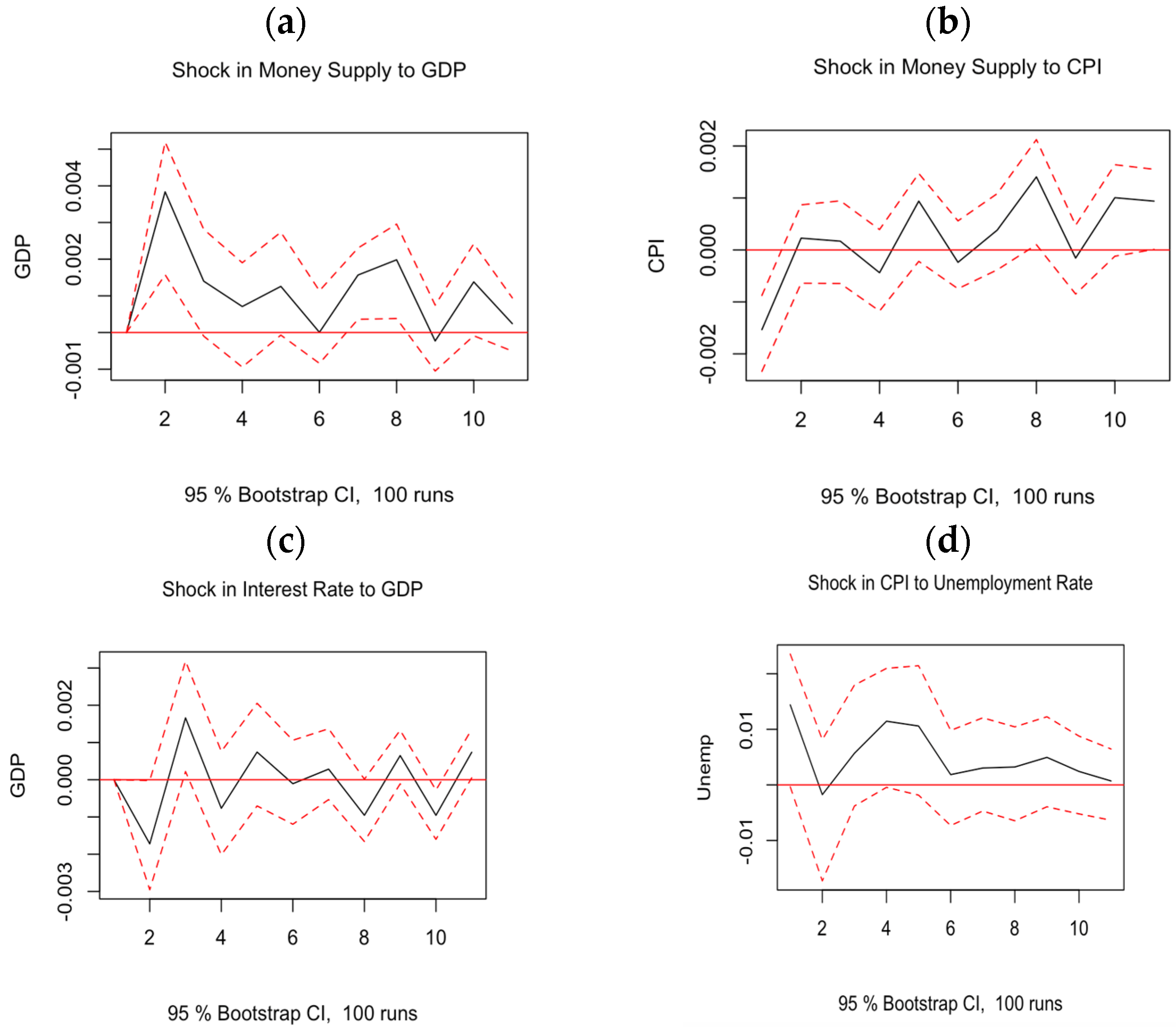
The VAR model is composed of 5 endogenous variables. Gross Domestic Product, Money Supply, Consumer Price Index, Interest Rate, and Unemployment Rate. This is Y = Ln(GDP), Ln(M2), Ln(CPI), Ln(IR), and Ln(Unemp), respectively. Where Ln is their logarithm to a constant base e. This approach shall allow us to conduct an impulse response analysis, which shows the impact of one standard deviation shock in one of the variables concerning another, e.g., one standard deviation change in M2 may cause a short- or long-term impact on GDP. Similarly, one standard deviation change in Interest Rate (IR) may affect the Unemployment Rate up or down.
In the following Section, we explore and expose the procedures and outcomes of the tests performed that support the conclusion in Section 4.

3. Data Analysis: Diagnoses and Data Preparation

This piece of work aims to empirically test the relationship between economic growth and monetary policy through a Vector Autoregressive model (VAR). In addition, Phillip’s assumption of inverse correlation between inflation and Unemployment Rate will be tested within the VAR model. According to the results of Table 1 and the high variability of the data shown by the standard deviation test, it is necessary to eliminate any possible trend or seasonality, which would violate the VAR assumptions. Therefore, the dataset was converted into a natural logarithm as shown in Figure 1.
Although the variables look smooth, there is an apparent trend for GDP and M2. Hence, a stationarity test is pivotal to test it and thus move on with the VAR methodology. The stationarity test performed here is the Augmented Dickey–Fuller, and the obtained results are reported in Table 2.
Therefore, apart from the Unemployment Rate, all other variables are non-stationary since the p-values are higher than 5% with a lag order of 6, which is the number of previous values in the autoregressive model that can be regressed. Thus, the result leads to accepting the null hypothesis of non-stationary. The p-value is a critical mechanism for testing the probability of rejecting a null hypothesis, as Thiese et al. [37] observed. Since GDP, M2, CPI, and IR are non-stationary, the alternative is to apply the differencing technique and thus stabilize the mean of the data. Although initially, the dataset looks stationary, it is crucial to rerun the ADF test as per Figure 2 and Table 2.
From Table 3, the Consumer Price Index (CPI) remains non-stationary. At the same time, the Gross Domestic Product (GDP), Interest Rate (IR), and Unemployment Rate are stationary with an α value of 1%, which is the level of statistical confidence. Furthermore, the scatterplot in Figure 3 precisely shows the behavior of each variable where the y-axis is the log value after applying differencing to remove the remaining, and the x-axis is the number of observations that are now stationary, apart from the Consumer Price Index (CPI). Such a non-stationary pattern is evident as the dots are a little dispersed from their mean (represented by a line in these subplots), which confirms the ADF result of non-stationary.

3.1. Vector Autoregressive Model Deployment

Hence, the VAR model can be applied to the dataset transformed from non-stationary to stationary. The software used for the analysis was R, and the first step was to declare the variables chosen to be analyzed. The variables are coded as time series from 1959 to 2022 with quarterly frequency as described. Then, the variables were bound within one vector to define the optimum lag length using the lag selection criteria applying the function ‘’VARselect’’ and considering a maximum lag length of 10 to avoid compromising the degrees of freedom. According to Table 4, the lag selection criteria options are Akaike Information Criterion (AIC) [38], Schwarz Information Criterion (SIC) [39], Hannan–Quinn (HQ) [40], and Final Prediction Error (FPE). The optimum lag length is four, the most frequent number among the selection criteria. Ivanov and Kilian [41] showed that AIC produces the most accurate impulse response for realistic sample sizes. It is worthwhile to mention, however, that as observed by Gujarati [31] that ‘there is no a priori guide to what is the maximum length of the lag’. However, he also points out that successive lag estimation reduces the degrees of freedom, which makes the statistical inferences more unstable. Once the lag length is defined, the VAR model can be built using the var function from the VARs library on lag 4 (p).
The VAR estimation results of GDP in relation to M2, IR, CPI, and Unemp is shown in Table 5.
We can see a sample size of 249 observations from a total of 253, and a difference is caused by the fact that four observations are the lags of the model. It is also important to note that the roots of the characteristic polynomial are lower than 1, which confirms that the model is stable. The first column in the table contains the correlated variables along and the related lag. The ‘Estimate’ refers to the estimated value based on the correlated variable and its lag. The ‘Standard Error’ is the standard deviation of the statistical sample. The ‘T value’ measures the estimated parameter value from the hypothesis value, the ‘p-value’ as mentioned before, measures the statistical significance, and finally, the ‘stars’ evidence the level of significance in descending order, 3 being the maximum level of statistical significance.
Looking closely at Table 5, we can see that the VAR estimation for GDP at lag 1, which is equivalent to 1 quarter of the past value of GDP along with M2. Also, the Unemployment Rate is statistically significant at an alpha (α) value of 5%, which is a threshold of the significance level that determines whether or not we can reject the null hypothesis. Therefore, a p-value larger than 0.05 or 5% would break the threshold leading to accepting the null hypothesis. The relationship between GDP and its past lag value remains on lag two, and the Interest Rate appears statistically significant and positively impacts GDP. In addition, the residual standard error of 0.01 shows the model’s accuracy as it is very close to 0. Furthermore, the adjusted R-squared of 24 shows that 24% of GDP variations are explained by its own past values plus M2, Unemployment Rate, and Interest Rate.
From Table 6, we can see a negative relationship between GDP and M2 for the first lag. This means that as GDP increases, the Money Supply decreases. Also, at lag 1, we can see Money Supply as a function of its previous values, but this relationship does not look consistent as M2 is not significant at lag 4. It is interesting to note that there is a significant positive relation between M2 and IR at lag 4, which is counter-intuitive at first glance, considering the latest FED’s expansive monetary policy approach, e.g., Quantitative Easing (Quantitative Easing is an expansionary monetary policy approach where the Federal Reserve buys bonds and assets from financial institutions to inject liquidity into the economy and thus avoid the solvency of banks and firms in the United States [42]).This suggests that monetary policy does not effectively impact Interest Rate in the short run. The residual standard error equals 0.004, which indicates that the model is accurate. The adjusted R squared illustrates the amount of variability in M2 equal to 41% is explained by variations in Gross Domestic Product (GDP), Consumer Price Index (CPI), Interest Rate (IR), and Unemployment Rate (Unemp), because the p-value is much less than 0.05, we can reject the null hypothesis of no association among the variables and accept the alternative hypothesis of association.
From Table 7, it is evident that the Consumer Price Index (CPI) appears to be related to GDP at lag 1 and 4, it is own past value at lag 1 and 3, and it is related to both GDP and the Money Supply at lag 4. The relationship between GDP growth and CPI is intuitive and explained by supply and demand. In other words, prices tend to increase when demand increases faster than supply to find the equilibrium point over time. Consumption is increasing faster than production. However, it is interesting to see the relationship between CPI and its own lagged value of one-quarter with some variation over time because CPI at lags 2 and 4 are insignificant. Thus, the hypothesis of inertial inflation shall not be considered (Inertial inflation refers to the concept of current inflation + expected future inflation, and usually caused when the prices of goods and services of the economy follow an indexation process, e.g., yearly house rent is adjusted based on the inflation index. Such phenomena are common in countries undergoing a hyperinflationary period, e.g., Brazil from 1970 to 1994—see [43]). The model is statistically significant at an α value of 1% because the p-value is less than 2.2 × 10⁻¹⁶, which is lower than 1%. Therefore, the null hypothesis of no association can be rejected. However, it is essential to mention that any statement in concerning CPI must be taken with extra care, as the data was not stationary, and thus, further analysis is required.
Table 8 shows the VAR estimation for the Interest Rate concerning GDP, M2, CPI, and Unemployment Rate. We can see a positive relationship between GDP and M2 at lag 1 of 5.11 and 2.96, respectively. What should be taken into consideration here is the negative relationship between IR and CPI: −3.99 at lag 2 and −4.87 at lag 4. There is an idea of Interest Rate (IR) as a tool to curb inflation, the result can be explained by the monetary theory; when the interest rate increases inflation decreases. Although the residual standard error is more significant than previously observed outputs, as it remains under 0, it should not be a concern at this stage.
The VAR estimation for the Unemployment Rate in Table 9 indicates a strong negative relationship (at −3.08 estimate) with GDP at lag 2 and its own lagged value (at −0.40 and −0.23), which is intuitive as the economy grows, the Unemployment Rate falls. Conversely, as the economy shrinks, the Unemployment Rate tends to increase because of low economic activity and lack of job creation. In addition, the model shows a relatively low residual standard error and an adjusted R squared of 56%, which means that 56% of Unemployment Rate variations are explained by GDP, M2, CPI, and IR. Therefore, based on the p-value of <0.01 or <1%, the null hypothesis of no association among the variables can be rejected with a 99% confidence level. In other words, the difference between the p-value and the confidence level states whether there is enough evidence against the null hypothesis. Hence, there is substantial evidence to reject the null hypothesis and accept the alternative association hypothesis. In addition, it is worth mentioning that, according to the VAR model above, the relationship between the Unemployment Rate and inflation does not seem to hold nowadays, but further investigation is required.

3.2. Residual Tests

The autocorrelation test from the serial function within the VARs package, designed to test for correlated errors, was also performed.
Table 10a–d shows the portmanteau test of residual autocorrelation, where the Chi-square of 163.38 measures the relationship among the residual with the degree of freedom of 150, whereas the p-value of 5% indicates no autocorrelation, which leads to accepting the null hypothesis of no autocorrelation. We also test for heteroscedasticity using the Autoregressive Conditional Heteroskedasticity (arch) test, which measures the volatility among the variables. In the case of heteroscedasticity [44] and, based on the p-value more significant than 5%, we can state that there is no evidence to reject the null hypothesis of no heteroscedasticity and therefore assume the model is homoscedastic. However, when the arch test is performed individually by separating each variable, we can see that only CPI shows signs of heteroscedasticity. It is also vital to test whether the residuals are normally distributed or not. We consider the following three normality tests: Jarque–Bera, Skewness, and Kurtosis. The tests indicate that the model’s residuals are not normally distributed; consequently, we could drop variables and rerun the model, seeking improvements in the result. However, because the main target of this paper is to identify the relationship between Money Supply (M2) and GDP growth, instead of predicting a future value, the violation of normally distributed residual should not compromise the main result. In addition, the model proposed here has proven to be homoscedastic, and the dataset was appropriately transformed, as proposed by Knief and Forstmeier [45], allowing the reader to trust the outcome of this paper. Furthermore, it is also pivotal to test for structural breaks, which tests whether there are structural breaks in the residuals of the model that could, in case of a positive result, cause abrupt changes in the variables over time. According to the graphs and considering the lines do not trespass the boundaries, the x-axis is the fluctuation process within one standard deviation, which is shown by the red horizontal lines at the top and bottom of each graph, and the y-axis is the time horizon expressed in percentage. Therefore, we can state that there are no structural breaks, see Figure 4.

3.3. Granger Causality Test

Although the VAR test has identified several relationships among the variables we analyzed, it is highly relevant to test for causality. Therefore, the Granger causality test was performed to accomplish such a goal.
From Table 11, we can see that the null hypothesis of the Granger causality test H0 is that GDP does not Granger cause M2, CPI, IR, and Unemp. The degree of freedom (df) refers to the dataset’s information to estimate the population’s unknown parameters. Therefore, according to the result, H0 can be rejected with a 99% confidence level. The same was found for instant Granger causality, which means that GDP does Granger cause M2, CPI, IR, and Unemp. Similarly, for M2, we also reject the null hypothesis of no Granger causality in the long and short term. Therefore, the result shows that M2 does instant Granger cause GDP, CPI, IR, and Unemp with a 99% confidence level. As for CPI, the test result shows a Granger causality in GDP, M2, IR, and Unemp for both the long and short term. The Granger causality test for Interest rate also indicates a Granger causality in GDP, M2, CPI, and Unemp. However, in the case of the Unemployment Rate (Unemp), the situation is somewhat different as the Unemployment Rate does not Granger cause GDP, M2, CPI, and IR for both the short and long term.

3.4. Impulse Response Function Test

The Granger causality test examined the relationship among the model variables, apart from the Unemployment Rate. However, an additional test required to evaluate the impact of the change in the monetary policy over time will be called “shock”. To do that, the impulse response function (IRF) from the vars library will be applied.
We can see from Figure 5a how a shock of one standard deviation in M2 would impact GDP considering 5 to 10 periods, more precisely, a change in the Money Supply by the Federal Reserve equivalent to one standard deviation in M2. However, it is pivotal to emphasize that since the dataset has been structured quarterly, one period represents one quarter. Therefore, ten periods are equal to two years and six months. Hence, one standard deviation shock in M2 would cause a positive response in the term but slowly ease off until it is almost zero. Figure 5b indicates a clear positive impact on the Inflation Rate measured by the CPI index for one standard deviation change in Money Supply (M2) in the long term. The effect of an expansionary monetary policy action would affect the CPI for as long as 30 months with a certain degree of variation but with an upward trend. For the Interest Rate Figure 5c, a shock of one standard deviation harms GDP for about three continuous periods; it is nine months before it shows any positive signs that do not last long. Therefore, IR does not effectively stimulate economic growth in the long run. Finally, Figure 5d illustrates that one standard deviation shock in CPI harms unemployment in the short run, but this negative relationship disappears in the long run.

4. Conclusions

When the Federal Reserve (FED) acts to provide liquidity in the market through expansionary monetary policy, it automatically generates debt because money is a liability and not an asset from the central bank’s perspective. Therefore, an increase in Money Supply (M2) comes at the cost of several implications, and among many, one stands out as being the most relevant, the currency trust. It is obvious how active the FED is whenever the United States faces threats to the entire financial system at the end of an economic cycle (e.g., subprime 2008 and the COVID-19 pandemic 2020). The data analysis section of this study suggests that monetary policy conducted by the Federal Reserve (FED) does cause an impact on Gross Domestic Product (GDP) growth in the short term as per the VAR output test (Table 5) as well as the Granger causality test (Table 11). Moreover, the Impulse Response Function (IRF) test confirmed the findings of instantaneous causality. Therefore, when the FED increases the Money Supply (M2) in the economy, the effect is immediate on GDP for the next quarter, but this is an artificial growth mainly caused by the liquidity excess in the market that lasts until this capital is allocated. This effect does not last long concerning economic growth, though it causes a long-term impact on the Consumer Price Index (CPI). The responsibility of the FED in generating an inflationary process has already been found; see Goodfriend [46]. Thus, monetary policy should be applied responsibly and with fiscal policy to ensure no long-term inflation, as observed by [47], maintaining the dollar stability as a global store of value currency. Furthermore, we found that M2 is affected by the Unemployment Rate at lag 2 and 4. However, if we consider the FED’s role, that is to promote production growth, maximize employment, maintain price stability, and moderate interest rates. Thus, it is expected that at the end of an economic cycle, the FED will need to act to protect and retain jobs in order to keep consumption constant and succeed in promoting economic growth. Currently, increasing the Money Supply in commercial banks will increase their reserves, allowing these institutions to lend at low interest rates to firms that need capital investments or merely to keep operating. However, when going through a financial crisis, firms and individuals are unlikely to acquire more debt, and even if a part of them does, if there is not enough demand for goods and services, the excess of liquidity in the economy would end up in financial bubbles. The IRF showed that Money Supply affects CPI in the short and long run. However, the VAR test is not statistically significant at an alpha value of <5% but an alpha value of 10% (Table 7). It is interesting to note that looking at Figure 1, we can see a sharp rise after 2019 in M2, which is the increase of Money Supply into the economy by the FED’s bond purchase scheme, but CPI has not increased accordingly in the same proportion. There could be several causes for this. The first is due to the uncertainty during financial crises; therefore, although there is more money in the economy, if uncertainty is high, households may avoid consumption while firms avoid investments, a situation already observed by [5,48]. Thus, the lack of consumption leads to low aggregate demand. The second reason is related to the first one, or perhaps, it is a consequence.
Hence, as consumption decreases, the money injected into the economy would become unproductive capital, which, in this case, only serves to cause asset inflation in the financial market. The VAR test for the Interest Rate showed a relationship with GDP growth at lag 2. The test also showed a negative relationship between Interest Rate and Consumer Price Index at different lags. It implies that the FED does respond to inflationary processes but is inconclusive in curbing inflation and promoting economic growth in the long run. Additionally, the Unemployment Rate has a statistically inverse relation with GDP growth at lags 2 and 3, which suggests that unemployment is affected by GDP. Based on this study, there is no relationship between unemployment and inflation. In this work, we measured inflation by studying the Consumer Price Index (CPI). However, it is worthwhile mentioning that there are other inflation indicators: such as the wholesale price index (WPI) and the producer price index (PPI). In future work, we will use machine learning network algorithms to model this economic application and compare the obtained results with this paper’s results.

Author Contributions

A.A.: conceptualization, investigation, software, formal analysis, visualization, data curation, writing—original draft, T.E.D.: conceptualization, methodology, investigation, resources, visualization, data curation, supervision, validation, writing—review and editing, H.A.A.: methodology, validation, review & editing, H.M.A.: validation, resources, project administration, funding acquisition, writing—review and editing. All authors have read and agreed to the published version of the manuscript.

Funding

This study was funded by Taif University Researchers Supporting Project number (TURSP-2020/279), Taif University, Taif, Saudi Arabia. Also, the APC was funded by the same sponsor.

Data Availability Statement

All of the data used in this study are available at the public repository https://fred.stlouisfed.org/series/M2SL (accessed on 2 November 2022).

Acknowledgments

We would like to thank Taif University Researchers Supporting Project number TURSP-2020/279, Taif University, Taif, Saudi Arabia, for funding this research.

Conflicts of Interest

The authors declare no conflict of interest.

References

  1. Federal Reserve Bank of New York. 2001. Available online: https://www.newyorkfed.org/aboutthefed/annual/annual01/index.html (accessed on 10 May 2021).
  2. Hayes, A. Open Market Operations (OMO). 2022. Available online: https://www.investopedia.com/terms/o/openmarketoperations.asp (accessed on 14 June 2022).
  3. Wallace, N. A Modigliani-Miller Theorem for Open-Market Operations. Am. Econ. Rev. 1981, 71, 267–274. [Google Scholar]
  4. Feldstein, M.; Stock, J. The Use of a Monetary Aggregate to Target Nominal GDP, Monetary Policy; The University of Chicago Press: Chicago, IL, USA, 1994; pp. 7–69. [Google Scholar]
  5. Keynes, J.M. The General Theory of Employment, Interest and Money; Harcourt, Brace: New York, NY, USA, 1936. [Google Scholar]
  6. Francis, N.R.; Jackson, L.E.; Owyang, M.T. How has Empirical Monetary Policy Analysis in the U.S. Changed after the Financial Crisis? Econ. Model. 2020, 84, 309–321. [Google Scholar] [CrossRef]
  7. Lhuissier, S.; Mojon, B.; Rubio, J. Bis.org. 2020. Available online: https://www.bis.org/publ/work855.pdf (accessed on 14 June 2022).
  8. Mitchell, C. Liquidity Trap: Definition, Causes, and Examples. 2020. Available online: https://www.investopedia.com/terms/l/liquiditytrap.asp (accessed on 14 June 2022).
  9. Pettinger, T. Liquidity Trap—Definition, Examples and Explanation, Economics Help. 2020. Available online: https://www.economicshelp.org/blog/1892/economics/liquidity-trap/ (accessed on 14 June 2022).
  10. Board of Governors of the Federal Reserve System, Federal Open Market Committee Announces Approval of Updates to Its Statement on Longer-Run Goals and Monetary Policy Strategy. 2020. Available online: https://www.federalreserve.gov/newsevents/pressreleases/monetary20200827a.htm (accessed on 14 June 2022).
  11. Board of Governors of the Federal Reserve System, What Economic Goals Does the Federal Reserve Seek to Achieve Through Its Monetary Policy? 2020. Available online: https://www.federalreserve.gov/faqs/what-economic-goals-does-federal-reserve-seek-to-achieve-through-monetary-policy.htm (accessed on 14 June 2022).
  12. Board of Governors of the Federal Reserve System, Available, Federal Reserve Board—Monetary Policy: What Are Its Goals? How Does It Work? 2021. Available online: https://www.federalreserve.gov/monetarypolicy/monetary-policy-what-are-its-goals-how-does-it-work.htm (accessed on 15 June 2022).
  13. Batrancea, L.; Rathnaswamy, M.K.; Batrancea, I. A Panel Data Analysis on Determinants of Economic Growth in Seven Non-BCBS Countries. J. Knowl. Econ. 2022, 13, 1651–1665. [Google Scholar] [CrossRef]
  14. Batrancea, L.; Rus, M.I.; Masca, E.S.; Morar, I.D. Fiscal Pressure as a Trigger of Financial Performance for the Energy Industry: An Empirical Investigation across a 16-Year Period. Energies 2021, 14, 3769. [Google Scholar] [CrossRef]
  15. Batrancea, L. An Econometric Approach Regarding the Impact of Fiscal Pressure on Equilibrium: Evidence from Electricity, Gas and Oil Companies Listed on the New York Stock Exchange. Mathematics 2021, 9, 630. [Google Scholar] [CrossRef]
  16. Batrancea, L. The Influence of Liquidity and Solvency on Performance within the Healthcare Industry: Evidence from Publicly Listed Companies. Mathematics 2021, 9, 2231. [Google Scholar] [CrossRef]
  17. Kamaan, K. The Effect of Monetary Policy on Economic Growth in Kenya. Int. J. Bus. Commer. 2014, 3, 11–24. [Google Scholar]
  18. Bernanke, B.; Bliner, A. The Federal Funds Rate and the Channels of Monetary Transmission. Am. Econ. Rev. 1992, 82, 901–921. [Google Scholar]
  19. Fisher, I. The Purchasing Power of Money. Its Determination and Relation to Credit Interest and Crises; Augustus M. Kelley: New York, NY, USA, 1911. [Google Scholar]
  20. Friedman, M. The Quantity Theory of Money—A Restatement; University of Chicago Press: Chicago, IL, USA, 1956. [Google Scholar]
  21. Cioran, Z. Monetary Policy, Inflation and the Causal Relation between the Inflation Rate and Some of the Macroeconomic Variables. Procedia Econ. Financ. 2014, 16, 391–401. [Google Scholar] [CrossRef] [Green Version]
  22. Bhattarai, K. Unemployment-inflation Tarde-offs in OECD Countries. Econ. Model. 2016, 58, 93–103. [Google Scholar] [CrossRef] [Green Version]
  23. Ball, L.; Leigh, D.; Loungani, P. Okun’s law: Fit at 50. J. Money Credit Bank. 2017, 49, 1413–1441. [Google Scholar] [CrossRef]
  24. Phillips, A. The Relation between Unemployment and the Rate of Change of Money Wage Rates in the United Kingdom, 1861–1957. Economica 1958, 25, 283–299. [Google Scholar] [CrossRef]
  25. Islam, M.; Hossain, E. Does the monetary policy have any short-run and long-run effect on economic growth? A developing and a developed country perspective. Asian J. Econ. Bank. 2022, 6, 26–49. [Google Scholar] [CrossRef]
  26. Bhar, R.; Malliaris, A.G. Modeling U.S. monetary policy during the global financial crisis and lessons for COVID-19. J. Policy Model. 2021, 43, 15–33. [Google Scholar] [CrossRef] [PubMed]
  27. Feldkircher, M.; Huber, F.; Pfarrhofer, M. Measuring the effectiveness of US monetary policy during the COVID-19 recession. Scott. J. Polit. Econ. 2021, 68, 287–297. [Google Scholar] [CrossRef]
  28. Lombardi, M.J.; Zhu, F. A shadow policy rate to calibrate US monetary policy at the zero lower bound. Int. J. Cent. Bank. 2014, 305–346, BIS Working Paper No. 452. [Google Scholar]
  29. Lombardi, M.J.; Zhu, F. A Shadow Policy Rate to Calibrate U.S. Monetary Policy at the Zero Lower Bound. IJCB Int. J. Cent. Bank, Ant Financial. 2018. Available online: https://www.ijcb.org/journal/ijcb18q4a8.htm (accessed on 15 June 2022).
  30. George, D.; Mallery, M. SPSS for Windows Step by Step: A Simple Guide and Reference, 10th ed.; Pearson: Boston, MA, USA, 2010. [Google Scholar]
  31. Gujarati, D. Basic Econometrics, 4th ed.; McGraw-Hill Companies: New York, NY, USA, 2014. [Google Scholar]
  32. Sims, C. Macroeconomics and Reality. J. Econ. Soc. 1980, 48, 1–48. [Google Scholar] [CrossRef] [Green Version]
  33. Luetkepohl, H. Vector Autoregressive Models; European University Institute, Florence Department of Economics: Fiesole, Italy, 2011. [Google Scholar]
  34. Salmanov, O.; Zaernjuk, V.; Lopatina, O.; Drachena, I.; Vikulina, E. Investing the Impact of Monetary Policy using the Vector Autoregression Method. Int. J. Econ. Financ. Issues 2016, 6, 273–282. [Google Scholar]
  35. Dickey, D.; Fuller, W. Distribution of the Estimators for Autoregressive Time Series with a Unit Root. J. Am. Stat. Assoc. 1979, 74, 427–431. [Google Scholar]
  36. Granger, C. Investigating Causal Relations by Econometric Models and Cross-spectral Methods. Econometric 1969, 37, 424–438. [Google Scholar] [CrossRef]
  37. Thiese, M.; Ronna, B.; Ott, U. P-value interpretations and considerations. J. Thorac. Dis. 2016, 8, E928–E931. [Google Scholar] [CrossRef] [PubMed] [Green Version]
  38. Akaike, H. Fitting Autoregressive Models for Prediction. Ann. Inst. Stat. Math. 1969, 21, 243–247. [Google Scholar] [CrossRef]
  39. Schwarz, G. Estimating the Dimension of a Model. Ann. Stat. 1978, 6, 461–464. [Google Scholar] [CrossRef]
  40. Hannan, E.J.; Quinn, B.G. The Determination of the Order of an Autoregression. J. R. Stat. Soc. 1979, 41, 190–195. [Google Scholar] [CrossRef]
  41. Ivanov, V.; Kilian, L. Studies in Nonlinear Dynamics & Econometrics. Stud. Nonlinear Dyn. Econom. 2005, 9, 1–36. [Google Scholar]
  42. William, S. Quantitative Easing: How Well Does This Tool Work? The Federal Reserve of Bank of St. Louis: St. Louis, MO, USA, 2017. [Google Scholar]
  43. Bresser-Pereira, L. A Descoberta da Inflacao Inercial. J. Contemp. Econ. 2010, 14, 167–192. [Google Scholar] [CrossRef] [Green Version]
  44. Engle, R. Autoregressive Conditional Heteroscedasticity with Estimates of the Variance of United Kingdom Inflation. Econometrica 1982, 50, 987–1007. [Google Scholar] [CrossRef]
  45. Knief, U.; Forstmeier, W. Violating the normality assumption may be the lesser of two evils. Behav. Res. 2021, 53, 2576–2590. [Google Scholar] [CrossRef]
  46. Goodfriend, M. The Inflation-Targeting Debate; University of Chicago Press: Chicago, IL, USA, 2004. [Google Scholar]
  47. Chari, V.V.; Kehoe, P. Optimal fiscal and monetary policy. Handbook of Macroeconomics. Elsevier 1999, 1, 1671–1745. [Google Scholar]
  48. Hicks, J.R. Mr. Keynes and the ‘Classics’; A Suggested Interpretation. Econometrica 1937, 5, 147–159. [Google Scholar] [CrossRef]
Figure 1. Macroeconomic variables in the log, over the examined period, 1959–2022.
Mathematics 10 04137 g001
Figure 2. Macroeconomic stationary variables.
Mathematics 10 04137 g002
Figure 3. Scatterplot of GDP, M2, CPI, IR, and Unemp.
Mathematics 10 04137 g003aMathematics 10 04137 g003b
Figure 4. Structural break test.
Mathematics 10 04137 g004
Figure 5. (a,b) Impulse Response Function (IRF) for Money Supply (M2) shock to Growth Domestic Product and shock to Consumer Price Index (CPI), respectively, (c) Impulse Response Function (IRF) for Interest Rate (IR) shock to Growth Domestic Product, and (d) Impulse Response Function (IRF) for Consumer Price Index shock to Unemployment.
Mathematics 10 04137 g005
Table 1. Descriptive Statistics.
Descriptive Statistics
GDPM2CPIIRUnemp Rate
Count254254254254254
Range24,372.5519,489.61259.6813.7511.4
Mean7875.34692.58131.334.555.97
Median6004.733224.5130.54.55.7
Std Dev45,722,788.122,441,850.666042.48.492.81
Skewness0.671.340.150.761.12
Kurtosis−0.791.07−1.320.742.49
Table 2. Augmented Dickey-Fuller test.
Augmented Dickey-Fuller Test
DataDickey–Fuller TestLag Orderp-ValueAlternative Hypothesis
GDP−0.3260.99Stationary
M2−1.5860.75Stationary
CPI−1.7360.69Stationary
IR−3.2460.08Stationary
Unemp−2.9960.15Stationary
Table 3. Augmented Dickey-Fuller test after stabilize the mean of data through applying the differencing technique.
Augmented Dickey-Fuller Test
DataDickey-Fuller TestLag Orderp-ValueAlternative Hypothesis
GDP−5.3560.01Stationary
M2−4.9960.01Stationary
CPI−2.8360.23Stationary
IR−5.8660.01Stationary
Unemp−6.2460.01Stationary
Table 4. Lag information criteria test.
Lag Information Criteria Test
Akaike Information Criterion—AICSchwarz Information Criterion—SCHannan–Quinn—HQFinal Prediction Error—FPE
4224
Table 5. The VAR estimation for Gross Domestic Product (GDP).
VAR Estimation Results
Endogenous variablesGDP, M2, CPI, IR, Unemp
Sample size249
Log likelihood4052.56
Max Roots of polynomial0.9367
VariablesEstimateStd. ErrorT valuePr(>|t|)Significance level
GDP—lag 10.240.082.940.00**
M2—lag 10.440.104.203.83 × 10−5***
Unemp—lag 10.010.00−2.430.01*
GDP—lag 20.180.092.040.04*
IR—lag 20.020.002.790.00**
Residual Std Error0.005 on 228 degrees of freedom
Multiple R-Squared0.30
Adjusted R-Squared0.24
F-statistic4.846 on 20 and 228 DF
p-value 8.674 × 10⁻¹⁰
Table 6. The VAR estimation of Money Supply (M2).
VAR Estimation Results
Endogenous variablesM2, GDP, CPI, IR, Unemp
Sample size249
Log-likelihood4052.56
VariablesEstimateStd. ErrorT valuePr(>|t|)Significance level
GDP—lag 1−0.240.06−3.690.00***
M2—lag 10.470.085.871.52 × 10−0***
Unemp—lag 10.020.013.100.00**
M2—lag 30.220.092.340.02*
IR—lag 40.010.012.120.03*
Residual Std Error0.004 on 228 degrees of freedom
Multiple R-Squared0.45
Adjusted R-Squared0.41
F-statistic9.53 on 20 and 228 DF
p-value <2.2 × 10⁻¹⁶
Table 7. VAR estimation of Consumer Price Index (CPI).
VAR Estimation Results
Endogenous variables GDP, M2, CPI, IR, Unemp
Sample size249
Log likelihood4052.56
VariablesEstimateStd. ErrorT valuePr(>|t|) Significance level
GDP—lag 11.26 × 10−14.27 × 1022.950**
CPI—lag 13.19 × 10−17.07 × 1004.511.05 × 10−5***
CPI—lag 31.97 × 10−17.36 × 1002.670.01**
GDP—lag 41.18 × 10−14.29 × 1002.740.01**
M2—lag 41.07 × 10−12.29 × 10−21.940.054
Residual Std Error0.00 on 228 degrees of freedom
Multiple R-Squared0.55
Adjusted R-Squared0.51
F-statistic14.09 on 20 and 228 DF
p-value <2.2 × 10⁻¹⁶
Table 8. VAR estimation for Interest rate (IR).
VAR Estimation Results
Endogenous variables GDP, M2, CPI, IR, Unemp
Sample size249
Log likelihood4052.56
VariablesEstimateStd. ErrorT valuePr(>|t|)
GDP—lag 15.111.393.680***
M2—lag 12.961.731.710.09
CPI—lag 2−3.992.36−1.690.09
IR—lag20.270.12.720.01**
M2—lag3−5.072.03−2.490.01*
CPI—lag 4−4.872.31−2.110.04*
Residual Std Error0.08 on 228 degrees of freedom
Multiple R-Squared0.19
Adjusted R-Squared0.11
F-statistic2.61 on 20 and 228 DF
p-value 0.001
Table 9. VAR estimation for the Unemployment rate (Unemp).
VAR Estimation Results
Endogenous variables GDP, M2, CPI, IR, Unemp
Sample size249
Log likelihood4052.56
VariablesEstimateStd. ErrorT valuePr(>|t|)Significance level
M2—lag 11.070.782.710**
IR—lag 10.120.052.140.03*
Unemp—lag 1−0.470.06−6.075.55 × 10−9***
GDP—lag 2−3.080.81−3.80.00***
CPI—lag 22.531.321.920.06.
IR—lag 2−0.360.06−6.341.23 × 10−9***
Unemp—lag 2−0.230.07−3.30.00 × 100**
GDP—lag 3−1.660.83−1.990.05*
M2—lag 4−21−20.05*
IR—lag 4−0.110.06−1.817.00 × 10−2.
Residual Std Error0.04 on 228 degrees of freedom
Multiple R-Squared0.59
Adjusted R-Squared0.56
F-statistic17.01 on 20 and 228 DF
p-value<2.2 × 10⁻¹⁶
Table 10. (a) Portmanteau test output, (b) Autoregressive Conditional Heteroskedasticity, (c) Autoregressive Conditional Heteroskedasticity test per variable, and (d) Normality test of residuals.
(a)
Portmanteau Test (Asymptotic)
DataResiduals of VAR_Model
Chi-squared163.38
df150
p-value0.21
(b)
ARCH Test (Multivariate)
DataResidual of VAR_Model
Chi-squared3428.1
df3375
p-value0.2575
(c)
ARCH Test (Univariate)
DataChi-Squareddfp-Value
GDP8.8428160.9197
M22.351161
CPI40.416160.00
IR4.0161160.9989
Unemp19.589160.2393
(d)
Normality Tests (Multivariate)
DataTestChi-Squareddfp-Value
ResidualsJB7234.510<2.2 × 10⁻¹⁶
ResidualsSkewness358.165<2.2 × 10⁻¹⁶
ResidualsKurtosis6876.45<2.2 × 10⁻¹⁶
Table 11. Granger causality test for Growth Domestic Product.
Granger Causality Test
DataVariabledf1df2p-ValueNull Hypothesis (H0)
VAR_modelGDP1611403.936 × 10−7GDP does not Granger cause M2, CPI, IR, and Unemp
VAR_modelM21611401.174 × 10−6M2 does not Granger cause GDP, CPI, IR, and Unemp
VAR_modelCPI1611400.00014CPI does not Granger cause GDP, M2, IR, and Unemp
VAR_modelIR1611402.071 × 10−9IR does not Granger cause GDP, M2, CPI, and Unemp
VAR_modelUnemp1611400.1308Unemp does not Granger cause GDP, M2, CPI, and IR
Instantaneous Granger Causality Test
DataVariabledf1p-ValueNull Hypothesis (H0)
VAR_modelGDP43.109 × 10−14No instantaneous causality between: GDP and M2, CPI, IR, and Unemp
VAR_modelM242.276 × 10−14No instantaneous causality between: M2 and GDP, CPI, IR, and Unemp
VAR_modelCPI41.13 × 10−7No instantaneous causality between: CPI and GDP, M2, IR, and Unemp
VAR_modelIR4<2.2 × 10⁻¹⁶No instantaneous causality between: IR and GDP, M2, CPI, and Unemp
VAR_modelUnemp40.4988No instantaneous causality between: IR and GDP, M2, CPI, and Unemp
Publisher’s Note: MDPI stays neutral with regard to jurisdictional claims in published maps and institutional affiliations.

