
On the Effects of Boundary Conditions in One-Dimensional Models of Hemodynamics


Faculty of Applied Mathematics and Control Processes, Saint Petersburg State University, 7/9 Universitetskaya Nab., 199034 Saint Petersburg, Russia
Mathematics 2022, 10(21), 4058; https://doi.org/10.3390/math10214058
Submission received: 9 October 2022
/
Revised: 26 October 2022
/
Accepted: 28 October 2022
/
Published: 1 November 2022
(This article belongs to the Special Issue Mathematical Modeling and Data Science for Biology and Medicine)
Abstract
:The paper is devoted to the theoretical analysis of the effects of boundary conditions on the solutions of the system of one-dimensional (1D) hemodynamics. The integral inequalities, which realize the energy inequalities for the solutions of initial-boundary-value problems, are obtained. It is demonstrated that the unphysical unbounded solutions can take place for the case of bounded functions from boundary conditions. For the periodic boundary conditions, the integral estimation illustrates the correct behavior of the solution. For this case of boundary conditions, the effective Fourier method for the analytical solution is proposed. The analytical solutions, obtained by this approach, can be used for the comparison of different 1D blood-flow models. The results obtained in the paper allow for an the alternatively view of the stated boundary conditions and can explain some problems, which can arise in numerical simulations. They expand the possibilities of the application of analytical methods in the field of blood-flow simulation. The results can be useful for the specialists on blood-flow modeling.
1. Introduction
Nowadays, the mathematical models of blood flow are widely used in applied medical investigations as a powerful tool for the prediction of the results of surgeries and different vascular defects (such as stenoses and aneurysms) [1,2]. For the simulation of processes in large vascular systems, 1D models are widely used in practice [3,4]. These models are obtained by the averaging of the Navier—Stokes equations on the vessel cross-section [5,6,7]. As a result, the model based on the hyperbolic nonlinear system of 1D equations on the cross-sectional area and flow rate (or mean velocity) is constructed. These models can be coupled with 0D and 3D models [8], and the obtained results are close to the averaged solutions of 3D models [9].
From the physical viewpoint, blood is considered as an incompressible viscous fluid [10]. In most works, the viscosity of blood is described by the Newtonian model with the proper representation of the velocity profile [5,7,8,11]. However, in many works [12,13,14,15,16,17,18,19] the viscosity is ignored, and blood is considered as an inviscid fluid. This approximation can be used for the case of large arteries and veins, where the viscosity is not as important as it is in small vessels.
In recent decades, 1D models have been used for the simulation of many processes in physiology and medicine. For example, they have been applied to the simulation of system partial hepatectomy [3]; brain hemodynamics predictions [6,20]; the simulation of flow in large arteries [9] and near bifurcations [8]; the modelling of flows in systems with stenosed vessels [21]; the analysis of blood-flow effects on cerebrospinal fluid dynamics [22]; the analysis of flows in tapered vessels [23]; and the simulation of flows in arterial systems [24,25,26]. It must be noted that the results of the simulations are close to the results of the experiments (e.g., see [24,25]). Unfortunately, according to the nonlinear nature of the main equations, the different problems for such models in the general case can be solved only numerically. However, analytical methods are also actual in qualitative investigations of 1D hemodynamics because they can be used for the analysis of the qualitative properties of the solution (such as stability, dispersion, dissipation, etc.); for the comparison of different rheological models of blood; and for providing an effective tool for testing programs, which implement the algorithms of numerical methods [27].
The presented paper is devoted to the analytical investigation of possible qualitative properties of the solutions of 1D models of blood flow. It must be noted that investigations of this kind are presented in a relatively small number of works. For example, in the papers of Ashmetkov et al. [28,29], the linearized system for pressure and velocity is considered, and the method for the obtaining of analytical solutions, based on the reflection of waves, is proposed. Paquerot and Remoissenet [30] present a nonlinear model for the description of pressure-wave propagation in arteries. The model leads to the solution of the Boussinesq-type scalar equation. The one-soliton and two-soliton solutions, obtained by the Hirota method, are analyzed. Ilyin in [31] construct the model, based on the inviscid Burgers equation, and apply the method of characteristics for the solution of an initial-boundary-value problem on the semi-infinite interval in order to obtain the nonlinear pressure–velocity relations. Canic et al. [7] present the proof of the theorem, which provides the condition of the existence of a smooth global solution of a nonlinear conservative law system, and provide the conditions for the shock formation. The recent work [32] is devoted to the analysis of the well-posedness of the system of 1D equations in a network in the case of the vessels with viscoelastic properties. The conditions of the existence and uniqueness of the maximal strong solution are obtained, such as the stability estimations.
In the presented paper, we try to expand the field of application of analytical methods in the analysis of 1D blood-flow models and to demonstrate that the problems for linearized 1D system of inviscid hemodynamics can have physically irrelevant (unbounded) solutions for the physically relevant (bounded) boundary conditions. It is demonstrated that for the periodic conditions, this problem is not observed. For this case of boundary conditions, the simple and effective Fourier method is proposed.
2. Model
The 1D model of the inviscid blood flow in a distensible vessel with impermeable walls is based on the averaged incompressibility condition and momentum equation [6,31]:
where t is a time, z is a cylindrical coordinate, is the cross-sectional area, is the flow rate (, where U is the mean axial velocity), is the pressure, and is a constant density.
System (1) is closed by the equation-of-state . In the case of the arteries, the following equation is used [6,9]:
where is the external pressure; and are the diastolic pressure and cross-sectional area; , where E is the Young’s modulus; and h is the vessel wall thickness. In the paper, the case of constant values of , , E, and h is considered.
Let the following dimensionless variables be introduced:
where , , , are the characteristic length, time, cross-sectional area, and velocity. The value of is considered as a vessel length, can be estimated by the maximal wave speed, is computed from and , and can be estimated, for example, from the diastolic cross-sectional radius. The tilde sign in (4) will be ignored in the text below.
The interesting results on the solutions of the initial-boundary-value problems for (5) can be demonstrated for the linearized version of this system. For the linearization, we represent the solution of (5) as , , where is the constant steady-state solution of (5), and , are the small perturbations, as their first derivatives.
It must be noted that the speed of sound is presented as [9]: . So, , and in the dimensionless variables it is written as . At the same time, . The blood flow in physiological conditions is realized when [33], so the coefficient in (6) is strictly positive.
Let the single blood vessel, corresponding to the spatial interval be considered, and the following initial and boundary conditions are stated for (6):
where , , , are the known coefficients, and , , and , , , are the known functions, which are smooth enough. To ensure the smoothness of solution in , the following compatibility conditions are imposed:
3. Results
In this section, the integral inequalities, which provide the energy estimates of the solutions of (6)–(8), are obtained in order to demonstrate that the condition (9) can be broken.
As can be seen, and . Without the loss of generality, let the case of be considered, so , and we obtain that .
The matrix can be presented as , where is the diagonal matrix of eigenvalues and , are the matrices of left and right eigenvectors of , respectively.
Theorem 1.
Let the linear function be presented as
where , and the following inequalities are realized:
where
where are the components of matrix .
Then, the following inequality takes place:
where
and are the components of matrix .
Proof
(Proof). We introduce the new variables , as: , and according to the fact that , system (6) is rewritten as:
where , .
The initial and boundary conditions are rewritten as
where
The following new variables are introduced:
It must be noted that function with properties (11) can be selected for any finite values of and .
So, the Equation (13) are rewritten as
where . The initial and boundary conditions are rewritten as
where
We consider some functions , , and let the following relation take place for : , where . It is easy to demonstrate that , so . With the use of this inequality we obtain that
and according to the condition (see (11)), the following inequality can be written:
and by the same way, we obtain that
It is easy to demonstrate that
So, the following inequality is written:
With the use of the expression for and the integral mean value theorem, the following inequality can be obtained:
So, the following estimation takes place:
So, as we can see, according to (12), the problem (6)–(8) can have solutions, which are unbounded at , even though the bounded functions and are considered, and the physically relevant condition (9) may not be realized.
3.1. Case of Boundary Conditions for q
It must be noted that for the special classes of boundary conditions, the integral extimations, which are different from (12), can be obtained. LWe consider system (6) with initial conditions (7) and the following boundary conditions:
Theorem 2.
Let , . Then, the following integral inequality takes place:
Proof.
The new function, which satisfies the boundary condition (20), is introduced:
System (22) is considered with the following initial and boundary conditions:
where . So, the inhomogeneous system (22) with the homogeneous boundary conditions for is considered. According to the Duhamel’s principle [34], the solution of this problem can be presented as
where is the solution of the following problem:
and is the solution of the following problem:
We obtain the expression for the time derivative of :
where the boundary conditions (25) are taken into account.
So, we can obtain the following:
After the integration, the following equality is obtained:
By the same operations we obtain
According to Equation (23):
From we can obtain
and the following inequality can be written:
The same inequality takes place for .
So, the following estimation is obtained:
According to the Cauchy–Schwarz inequality, we obtain
As we can see, the last terms in (21) provide the possibility of the time-growing solutions for the bounded physically relevant functions and . We construct the simple example, which illustrates this behavior. Let and be the constants , , . Let , where D = . Let . This problem has the following solution:
So we can see that constant boundary conditions and bounded initial conditions lead to the unbounded unphysical () solution.
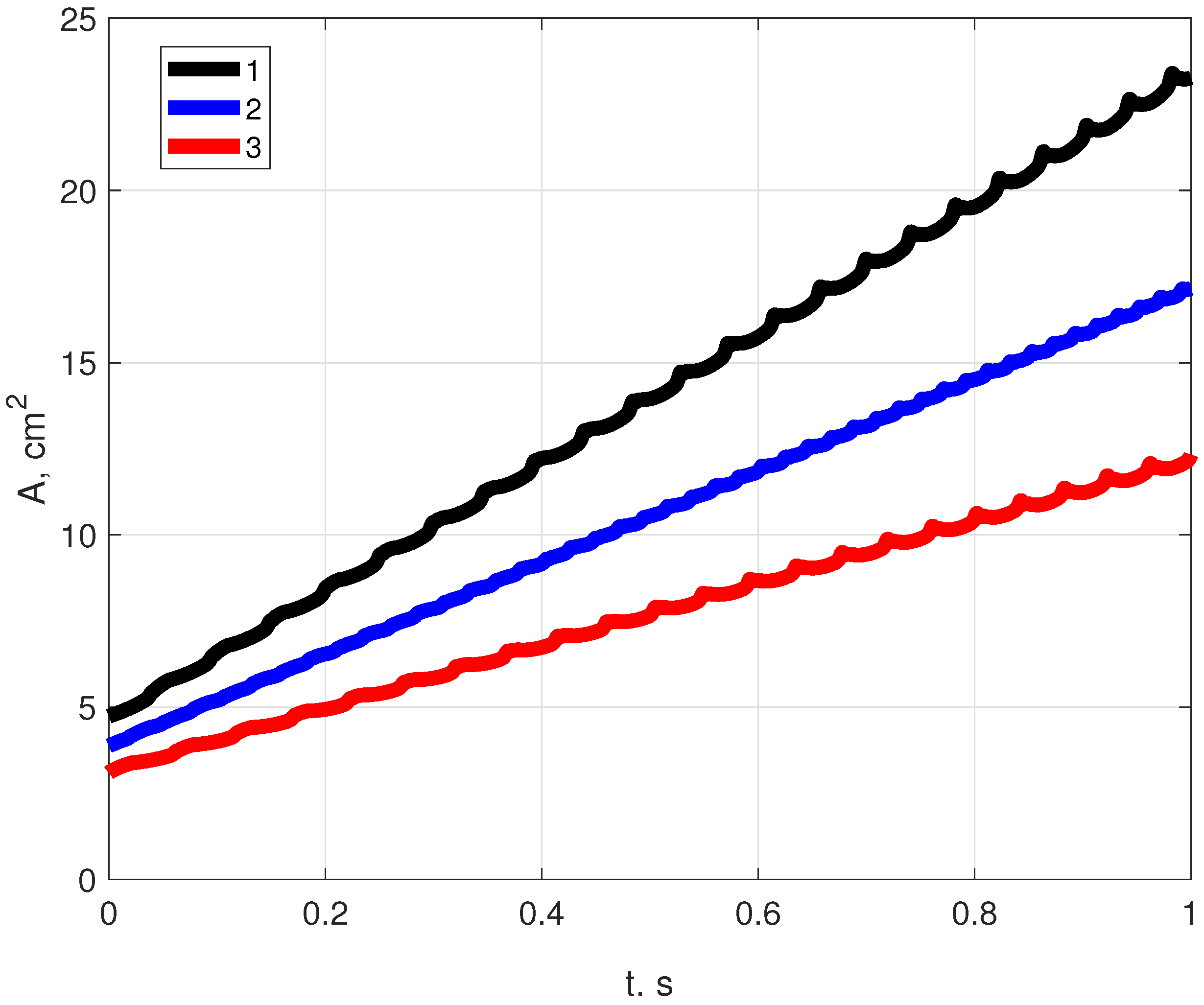
In order to demonstrate the similar behavior in the fully nonlinear model (1), which is widely used in practice, the physiological example on the simulation of blood flow in the part of the human aorta can be considered. For the simulation, the segment Ao. V from aortic model, presented in [9], is chosen. For this case, the variable mechanical properties take place: , . For this vessel, 15.2 cm, the radius of the inlet cross-section is equal to 1.25 cm, and the radius of the outlet cross-section is equal to 0.99 cm. The is chosen as
The values of for inlet and outlet cross-sections are computed from the values of the speed of sound, presented in Table IV from [9], and is considered as a linear function: .
The following boundary conditions are stated: , , which are close to the typical values of Q from [9]. The initial conditions are stated as
The numerical simulations are realized on the time interval from 0 to 1 s. The second-order Lax–Wendroff scheme is used for the computations on the spatial grid with 100 nodes and the time grid with 10,000 nodes. The values of A in the boundary points are computed from the compatibility conditions (for details, see [26]).
In Figure 1, the results of the numerical simulations are presented. As can be seen from the plots of A in the left, middle, and right vessel points, for this type of bounded boundary and the initial conditions, the obtained solutions do not have any physical or physiological meaning because they lead to the unbounded values of A. So, for this practical example we have the same behavior as for the linear theory.
3.2. Case of Periodic Boundary Conditions
We consider the following periodic boundary conditions for the system (6):
with the same initial conditions, but it is proposed that and .
3.2.1. Integral Estimation
Proof.
We obtain the expressions for :
so ,
So, we obtain that
3.2.2. Fourier Method
As is mentioned in the Introduction, the approach to obtain the solution of the initial-boundary-value problem for system (6) in the general form is proposed in [28,29], and it is based on the reflection of waves. In the case of periodic conditions (30), the Fourier method can be easily and effectively used.
Let the solution of system (6) be presented as
So, we obtain the following eigenvalue problem:
Problem (33) has the following eigenfunctions and corresponding eigenvalues:
The solution to the problem with periodic conditions (30) is presented as Fourier expansions on these eigenfunctions:
The solutions of (35) are presented as
where , and and are the constants. For we obtain that , , where and are the constants.
The constants in the expressions for and are defined after the substitution of (34) into initial conditions (7), expanded in the Fourier series on eigenfunctions of (33):
where
After this operation, the following expressions for constants are obtained:
We consider the following example: let , and the initial functions are presented as , , where . So, we obtain the following values of constants:
For this example, and are the real functions, written as
4. Discussion and Conclusions
In the presented paper, the author tries to expand the field of application of analytical methods in the simulation of blood flow and to analyze the effects of boundary conditions on the solutions of the linearized system of equations of 1D hemodynamics. The main results can be formulated as follows:
- The integral estimation (12) for the solution in the case of the general form of the boundary conditions is obtained. As can be seen, the unphysical unbounded solutions can take place for the case of bounded functions , .
- The general theory of the integral inequalities for hyperbolic equations is presented in [35,36]. However, in the presented paper, the more exact estimations are presented for the specific example of the hyperbolic system, where the specific constants in exponentials are obtained. Moreover, for the boundary conditions only for q, the estimation (21), which is more accurate than the exponential function (the linear function of t), is obtained.As it is mentioned in [36], the energetic norm is presented by the square of the -norm of the solution. In the left parts of (12), (21), and (32), the integrals, which can be considered as squares of norms of functions, linearly related to the solutions, are presented. So, our estimations can be considered as some kind of energy inequalities for this specific type of hyperbolic system with the appropriate boundary conditions.
- For the periodic boundary conditions, the exact integral estimation (31) is obtained, which illustrates the correct behavior of the solution—it is bounded at . For this case of boundary conditions, the Fourier method for the analytical solution can be applied. Such analytical solutions can be used for the comparison of different 1D blood-flow models [27].
- The results obtained in the paper can be useful for the specialists on blood-flow modeling because they allow for an alternative view of the stated boundary conditions and can explain some of the problems that can arise in numerical simulations.
- In the numerical experiment, where the fully nonlinear model, used in many works, is considered, it is demonstrated that the situation described by the author’s theoretical results can be observed in practice, when the bounded initial and boundary conditions lead to the incorrect results from the physical point of view. So, it is important to correctly impose the boundary conditions for the practical predictive simulations. From the medical point of view, this means that the users of the software must choose such conditions carefully because in the opposite case, it can lead to the incorrect results.
Funding
This research received no external funding.
Data Availability Statement
Not applicable.
Acknowledgments
The author wishes to thanks anonymous reviewers for the useful comments and discussion.
Conflicts of Interest
The author declares no conflict of interest.
References
- Sharifzadeh, B.; Kalbasi, R.; Jahangiri, M.; Toghraie, D.; Karimipour, A. Computer modeling of pulsatile blood flow in elastic artery using a software program for application in biomedical engineering. Comput. Methods Prog. Biomed. 2020, 192, 105442. [Google Scholar] [CrossRef] [PubMed]
- Karimipour, A.; Toghraie, D.; Abdulkareem, L.A.; Alizadeh, A.; Zarringhalam, M.; Karimipour, A. Roll of stenosis severity, artery radius and blood fluid behavior on the flow velocity in the arteries: Application in biomedical engineering. Med. Hypotheses 2020, 144, 109864. [Google Scholar] [CrossRef] [PubMed]
- Audebert, C.; Bucur, C.; Bekheit, M.; Vibert, E.; Vignon-Clementel, I.; Gerbeau, J. Kinetic scheme for arterial and venous blood flow, and application to partial hepatectomy modeling. Comput. Methods Appl. Mech. Eng. 2017, 314, 102–125. [Google Scholar] [CrossRef] [Green Version]
- Marchandise, E.; Willemet, M.; Lacroix, V. A numerical hemodynamic tool for predictive vascular surgery. Med. Eng. Phys. 2009, 31, 131–144. [Google Scholar] [CrossRef]
- Formaggia, L.; Lamponi, D.; Quarteroni, A. One-dimensional models for blood flow in arteries. J. Eng. Math. 2003, 47, 251–276. [Google Scholar] [CrossRef]
- Toro, E.F. Brain venous haemodynamics, neurological diseases and mathematical modelling. A review. Appl. Math. Comput. 2015, 272, 542–579. [Google Scholar] [CrossRef]
- Canic, S.; Kim, E.H. Mathematical analysis of the quasilinear effects in a hyperbolic model blood flow through compliant axi-symmetric vessels. Math. Methods Appl. Sci. 2003, 26, 1161–1186. [Google Scholar] [CrossRef]
- Dobroserdova, T.; Liang, F.; Panasenko, G.; Vassilevski, Y. Multiscale models of blood flow in the compliant aortic bifurcation. Appl. Math. Lett. 2019, 93, 98–104. [Google Scholar] [CrossRef]
- Xiao, N.; Alastruey, J.; Figueroa, C. A systematic comparison between 1-D and 3-D hemodynamics in compliant arterial models. Int. J. Numer. Methods Biomed. Eng. 2014, 30, 203–231. [Google Scholar] [CrossRef] [Green Version]
- Caro, C.G.; Pedley, T.J.; Schroter, R.C.; Seed, W.A. The Mechanics of the Circulation, 2nd ed.; Cambridge University Press: Cambridge, UK, 2011. [Google Scholar]
- Puelz, C.; Canic, S.; Riviere, B.; Rusin, C.G. Comparison of reduced models for blood flow using Runge—Kutta discontinuous Galerkin methods. Appl. Numer. Math. 2017, 115, 114–141. [Google Scholar] [CrossRef]
- Bertaglia, G.; Caleffi, V.; Valiani, A. Modeling blood flow in viscoelastic vessels: The 1D augmented fluid-structure interaction system. Comput. Methods Appl. Mech. Eng. 2020, 360, 112772. [Google Scholar] [CrossRef] [Green Version]
- Britton, J.; Xing, Y. Well-balanced discontinuous Galerkin methods for the one-dimensional blood flow through arteries model with man-at-eternal-rest and living-man equilibria. Comput. Fluids 2020, 203, 104493. [Google Scholar] [CrossRef]
- Favorskii, A.P.; Tygliyan, M.A.; Tyurina, N.N.; Galanina, A.M.; Isakov, V.A. Computational modeling of the propagation of hemodynamic impulses. Math. Models Comput. Simul. 2010, 2, 470–481. [Google Scholar] [CrossRef]
- Sheng, W.; Zheng, Q.; Zheng, Y. The Riemann problem for a blood-flow model in arteries. Commun. Comput. Phys. 2020, 27, 227–250. [Google Scholar] [CrossRef]
- Spiller, C.; Toro, E.F.; Vazquez-Cendon, M.E.; Contarino, C. On the exact solution of the Riemann problem for blood flow in human veins, including collapse. Appl. Math. Comput. 2017, 303, 178–189. [Google Scholar] [CrossRef]
- Toro, E.F.; Siviglia, A. Flow in collapsible tubes with discontinuous mechanical properties: Mathematical model and exact solutions. Commun. Comput. Phys. 2013, 13, 361–385. [Google Scholar] [CrossRef] [Green Version]
- Toro, E.F.; Muller, L.O.; Siviglia, A. Bounds for wave speeds in the Riemann problem: Direct theoretical estimates. Comput. Fluids 2020, 209, 104640. [Google Scholar] [CrossRef]
- Wang, Z.; Li, G.; Delestre, O. Well-balanced finite difference weighted essentially non-oscillatory schemes for the blood-flow model. Int. J. Numer. Meth. Fluids 2016, 82, 607–622. [Google Scholar] [CrossRef] [Green Version]
- Mohammad, S.; Hessam, B.; Kaveh, L. Physics-informed neural networks for brain hemodynamic predictions using medical imaging. IEEE Trans. Med. Imaging 2022, 41, 2285–2303. [Google Scholar]
- Pfaller, M.R.; Pham, J.; Verma, A.; Pegolotti, L.; Wilson, N.M.; Parker, D.W.; Yang, W.; Marsden, A.L. Automated generation of 0D and 1D reduced-order models of patient-specific blood flow. Int. J. Numer. Meth. Biomed. Eng. 2022, 38, e3639. [Google Scholar] [CrossRef]
- Toro, E.F.; Celant, M.; Zhang, Q.; Contarino, C.; Agarwal, N.; Linninger, A.; Muller, L.O. Cerebrospinal fluid dynamics coupled to the global circulation in holistic setting: Mathematical models, numerical methods and applications. Int. J. Numer. Meth. Biomed. Eng. 2022, 38, e3532. [Google Scholar] [CrossRef] [PubMed]
- Abdullateef, S.; Mariscal-Harana, J.; Khir, A.W. Impact of tapering of arterial vessels on blood pressure, pulse wave velocity, and wave intensity analysis using one-dimensional computational model. Int. J. Numer. Meth. Biomed. Eng. 2021, 37, e3312. [Google Scholar] [CrossRef] [PubMed] [Green Version]
- Matthys, K.S.; Alastruey, J.; Peiro, J.; Khir, A.W.; Segers, P.; Verdonc, P.R.; Parker, K.H.; Sherwin, S.J. Pulse wave propagation in a model human arterial network: Assessment of 1-D numerical simulations against in vitro measurements. J. Biomech. 2007, 40, 3476–3486. [Google Scholar] [CrossRef] [PubMed]
- Alastruey, J.; Khir, A.W.; Matthys, K.S.; Segers, P.; Sherwin, S.J.; Verdonc, P.R.; Parker, K.H.; Peiro, J. Pulse wave propagation in a model human arterial network: Assessment of 1-D visco-elastic simulations against in vitro measurements. J. Biomech. 2011, 44, 2250–2258. [Google Scholar] [CrossRef] [PubMed]
- Krivovichev, G.V. Computational analysis of one-dimensional models for simulation of blood flow in vascular networks. J. Comput. Sci. 2022, 62, 101705. [Google Scholar] [CrossRef]
- Krivovichev, G.V. Comparison of inviscid and viscid one-dimensional models of blood flow in arteries. Appl. Math. Comput. 2022, 418, 126856. [Google Scholar] [CrossRef]
- Ashmetkov, I.V.; Mukhin, S.I.; Sosnin, N.V.; Favorskii, A.P.; Khrulenko, A.B. Analysis and comparison of some analytic and numerical solutions of hemodynamic problems. Differ. Equ. 2000, 36, 1021–1026. [Google Scholar] [CrossRef]
- Ashmetkov, I.V.; Mukhin, S.I.; Sosnin, N.V.; Favorskii, A.P. A boundary value problem for the linearized haemodynamic equations on a graph. Differ. Equ. 2004, 40, 94–104. [Google Scholar] [CrossRef]
- Paquerot, J.-F.; Remoissenet, M. Dynamics of nonlinear blood pressure waves in large arteries. Phys. Lett. A 1994, 194, 77–82. [Google Scholar] [CrossRef]
- Ilyin, O. Nonlinear pressure-velocity waveforms in large arteries, shock waves and wave separation. Wave Motion 2019, 84, 56–67. [Google Scholar] [CrossRef] [Green Version]
- Maity, D.; Raymond, J.-P.; Roy, A. Existence and uniqueness of maximal strong solution of a 1D blood flow in a network of vessels. Nonl. Anal. Real World Appl. 2022, 63, 103405. [Google Scholar] [CrossRef]
- Mukhin, S.I.; Menyailova, M.A.; Sosnin, N.V.; Favorskii, A.P. Analytic study of stationary hemodynamic flows in an elastic vessel with friction. Differ. Equ. 2007, 43, 1011–1015. [Google Scholar] [CrossRef]
- Tikhonov, A.N.; Samarskii, A.A. Equations of Mathematical Physics; Dover Publications Inc.: New York, NY, USA, 1990. [Google Scholar]
- Godunov, S.K. The Equations of Mathematical Physics; Nauka: Moscow, Russia, 1979. (In Russian) [Google Scholar]
- Lax, P.D. Hyperbolic Partial Differential Equations; AMS: Providence, RI, USA, 2006. [Google Scholar]
Figure 1.
The values of the vascular cross-section in the chosen points: 1—; 2—; and 3—.

Publisher’s Note: MDPI stays neutral with regard to jurisdictional claims in published maps and institutional affiliations. |
© 2022 by the author. Licensee MDPI, Basel, Switzerland. This article is an open access article distributed under the terms and conditions of the Creative Commons Attribution (CC BY) license (https://creativecommons.org/licenses/by/4.0/).
Share and Cite
MDPI and ACS Style
Krivovichev, G.V. On the Effects of Boundary Conditions in One-Dimensional Models of Hemodynamics. Mathematics 2022, 10, 4058. https://doi.org/10.3390/math10214058
AMA Style
Krivovichev GV. On the Effects of Boundary Conditions in One-Dimensional Models of Hemodynamics. Mathematics. 2022; 10(21):4058. https://doi.org/10.3390/math10214058
Chicago/Turabian StyleKrivovichev, Gerasim V. 2022. "On the Effects of Boundary Conditions in One-Dimensional Models of Hemodynamics" Mathematics 10, no. 21: 4058. https://doi.org/10.3390/math10214058
Note that from the first issue of 2016, this journal uses article numbers instead of page numbers. See further details here.