Bayesian Inference for COVID-19 Transmission Dynamics in India Using a Modified SEIR Model

Abstract

We propose a modified population-based susceptible-exposed-infectious-recovered (SEIR) compartmental model for a retrospective study of the COVID-19 transmission dynamics in India during the first wave. We extend the conventional SEIR methodology to account for the complexities of COVID-19 infection, its multiple symptoms, and transmission pathways. In particular, we consider a time-dependent transmission rate to account for governmental controls (e.g., national lockdown) and individual behavioral factors (e.g., social distancing, mask-wearing, personal hygiene, and self-quarantine). An essential feature of COVID-19 that is different from other infections is the significant contribution of asymptomatic and pre-symptomatic cases to the transmission cycle. A Bayesian method is used to calibrate the proposed SEIR model using publicly available data (daily new tested positive, death, and recovery cases) from several Indian states. The uncertainty of the parameters is naturally expressed as the posterior probability distribution. The calibrated model is used to estimate undetected cases and study different initial intervention policies, screening rates, and public behavior factors, that can potentially strike a balance between disease control and the humanitarian crisis caused by a sudden strict lockdown.

1. Introduction

The outbreak of COVID-19 that first emerged in Wuhan, China, was declared a pandemic by the World Health Organization (WHO) on 11 March 2020 [1] since it quickly spread across the world. However, at the early stage, there was no vaccine, no cure, or approved pharmaceutical intervention, which made the fight against the pandemic reliant on non-pharmaceutical interventions (NPIs) [2]. These NPIs included macro-level approaches such as lockdown to reduce interpersonal contacts [3], and micro-level personal preventive measures such as physical distancing, mask-wearing, and personal hygiene [4,5,6], which aim to reduce the risk of transmission during contact with potentially infected individuals. Moreover, control measures employed in different countries and regions are different from partial closure (e.g., the transition from in-person classes to online classes, work from home, restrictions on social, sports, and cultural activities), travel ban, the shutdown of public transportation, to strict and complete shutdown (shelter in place order) [7,8,9,10]. While such an intense policy could reduce infection spread, it could give rise to severe social stress [11]. In particular, in India, the government imposed a strict lockdown on 25 March 2020, to slow down the initial outbreak at the early stage and to allow the public healthcare system to have some time and capacity to respond; however, the sudden lockdown soon turned into a humanitarian crisis. It left an enormous migrant population stranded in big cities and turned them into refugees overnight. Millions of migrant laborers started long journeys to return home by walking hundreds of miles. Before being hit by the virus, many lost their lives in different parts of the country as they tried to return home [12,13]. A retrospective analysis to compare the effect of these intervention strategies with other less extreme interventions on disease transmission dynamics is thus of great importance to our society.

In order to conduct such a retrospective analysis, it is essential to have a mathematical model that can accurately capture the disease transmission and progression dynamics in the target population. SEIR compartmental models are one of the widely used mathematical models in this context. Different versions of the classical SEIR methodology have been extensively studied and implemented for COVID-19 transmission dynamics in India [14,15,16,17] and across the world [8,18,19,20]. These traditional SEIR models only consider a single pathway for the disease progression, viz., susceptible stage to exposed or asymptotic infectious stage to symptomatic infectious stage to recovered stage. However, it is well known that for COVID-19 a section of the population never becomes symptomatic; instead, they recover from the asymptomatic stage directly. Thus, in our compartmental model, we include an additional disease progression pathway from susceptible to asymptomatic infectious to the recovered stage. In addition, most of these traditional approaches employ either a fixed transmission rate or a certain parametric time-dependent transmission rate from the susceptible to the exposed stage. As there are multiple factors that may affect this transmission rate, such fixed or simple time-dependent functions are not ideal for explaining the spread dynamics of such a complex disease. For this retrospective analysis in India, we propose a modified-SEIR model with a modified time-dependent transmission rate which depends on time through two factors, the contact rate or the proximity of individuals in the population and the change in personal behavior and personal hygiene. As the number of contacts among people decreases in proportion to the overall mobility during shutdown, it is reasonable to use the observed Google COVID-19 Community Mobility Report data [10] to approximate the effect of national lockdown in the disease transmission rate. The time-dependent transmission rate is thus expressed as a product of the initial normal transmission rate, the estimated mobility function, and a parametric sigmoid-type personal response function. The test rate and undetected cases are important features of COVID-19 different from other transmissible diseases, where a large number of secondary infections arise due to contact with undetected, pre-symptomatic, and asymptomatic cases. The existing SEIR literature, as mentioned above, does incorporate the available testing data into the compartmental model. One important aspect of our SEIR model is the use of publicly available testing data in estimating the transfer rate of each infectious compartment (symptomatic and asymptomatic) using testing data. We also model the cure rate and the mortality rate as time-dependent functions because it can be assumed that the health system improves its capability and techniques to cure infected patients over time. We use exponential models for both based on the empirical exploration of data.

Our retrospective analysis depends on the calibrated model parameters and the validation of the proposed model using the observed data. Traditional SEIR methodology uses an optimization method to estimate the unknown parameters of the model; however, here we focus on a Bayesian approach [21] which not only provides the estimates but also the corresponding uncertainties. The Bayesian approach proposes the solution as the posterior probability distribution of the parameters. It also regularizes the problem by incorporating the available information from other similar studies through prior distributions.

The spread of the virus in India was heterogeneous across states, which could be attributed to the different degrees of implementation of the central lockdown policy and citizens’ response for each state. Therefore, we selected five representative Indian states, namely, Maharashtra, Karnataka, Kerala, West Bengal, and Andhra Pradesh for the retrospective analysis. The proposed models are calibrated to daily COVID-19 data on daily infection, recovery, and death cases from mid-March to early December 2020 for these states. We partition the dataset into the training set to calibrate the model, and the validation set for prediction from the calibrated model. We also used mobility data for estimating the transmission rate and the testing data to estimate the rate of transition from the asymptomatic and symptomatic stages to the reported and quarantined stage. One of the goals of this retrospective study is to compare the various parameters of the fitted model across these states and analyze if the state-wise intervention policies have an effect on them. We also estimate and analyze the unknown undetected-to-detected cases ratio, which had a high impact on the COVID-19 pandemic duration and size. The percentage of symptomatic and asymptomatic cases is also estimated and analyzed together with their uncertainties. Assuming that isolation is successfully applied to the positive detected cases, undetected and asymptomatic cases would represent the primary source of infections. The estimated number of undetected and asymptomatic cases and their uncertainties could be critical for the public health decision-makers and individuals [22]. The other goal of the retrospective analysis is to study the effect of different intervention strategies on disease transmission dynamics using the calibrated model. In particular, we compared the possible effect of a few phase-wise less severe shutdown policies instead of a sudden complete shutdown, increased public awareness and personal protective measures such as mask-wearing, personal hygiene, and self-quarantine, and better testing and tracking policies, which can possibly balance the stress of migration workers and control the spread of the virus.

The article is organized as follows: in Section 2, we describe the modified SEIR dynamic model for the spread of COVID-19. The Bayesian inference methodology and the model calibration method are also discussed. We implement our methodology in Section 3 for the five representative states. Estimated parameters from different states are compared and their significance is discussed. The calibrated state models are used for retrospective analysis and to study the effect of different hypothetical control interventions. Section 4 concludes by summarizing our work and by discussing some future research directions.

2. Methodology

In this section, we first describe in detail the various aspects of the proposed modified SEIR compartment model to study the dynamics of COVID-19 transmission in India. Then, we describe the publicly available epidemiological data that are used for calibrating such model. Finally, we describe the Bayesian model calibration method and the corresponding Markov Chain Monte Carlo method used for the sampling-based inference.

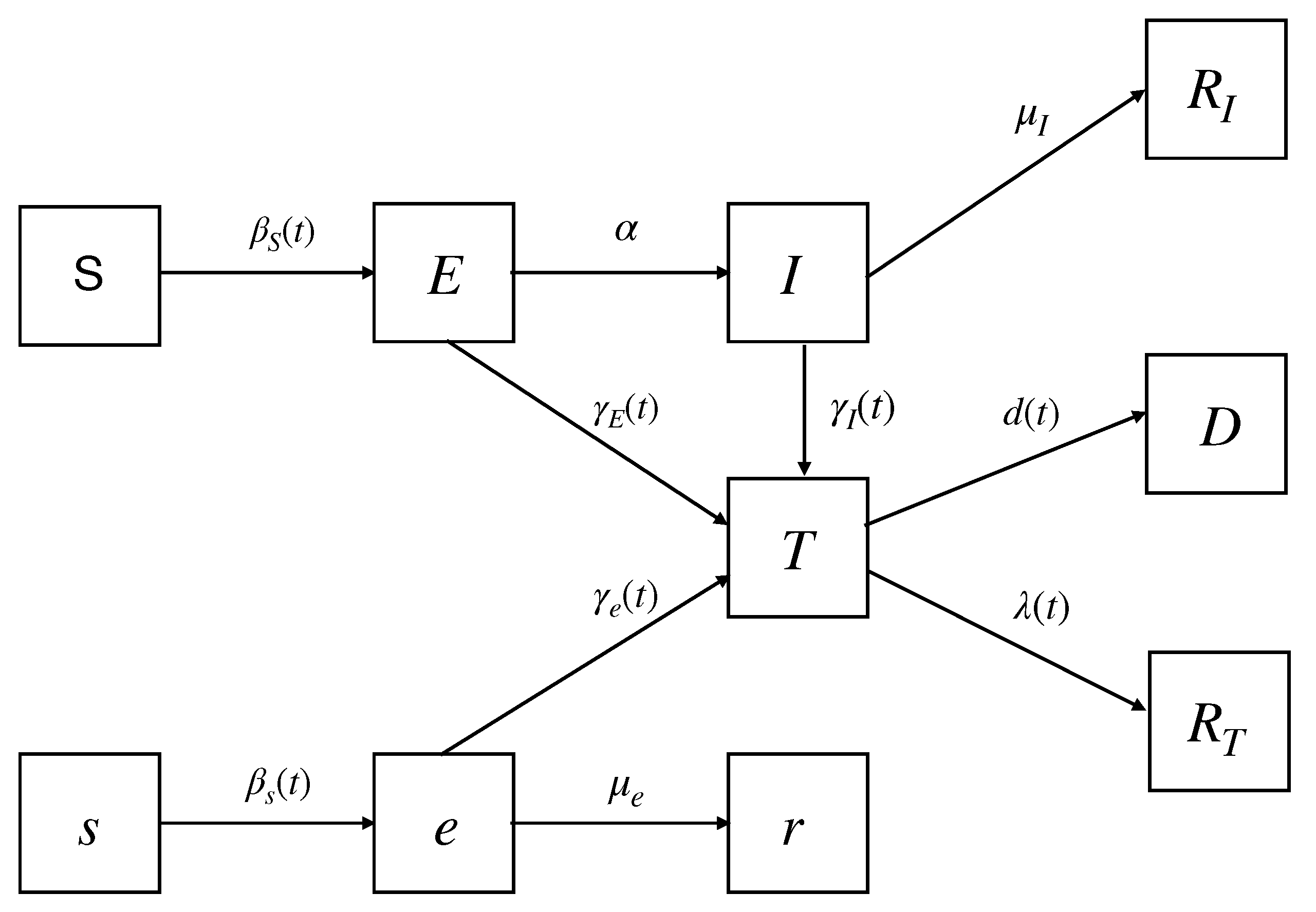
2.1. The Modified SEIR Model

Our model considers the following two different disease progression pathways from the susceptible (S and s) population: symptomatic ($S\to E\to I\to R$), and asymptomatic ($s\to e\to r$), as illustrated in Figure 1. The infection stages are classified as exposed (E and e), and infected but not reported as positive (I). Unlike other infectious diseases, asymptomatic individuals infected with COVID-19 can transmit the virus, so we include E and e among the infected stages. The non-infected stages are classified as symptomatic recovered but not reported $\left(R_I\right)$, asymptomatic recovered but not reported (r), infected and tested positive (T), death (D), and recovered $\left(R_T\right)$ from positive cases. To strike a balance between identifiable parameters and model completeness, we make a conservative assumption that all reported deaths caused by COVID-19 come from the T compartment. We also account for test screening and assume that all tested positive cases are quarantined or isolated and thus excluded from the transmission.

Taking into account the effects of mobility changes over time and personal behavior changes (frequent hand washing, wearing a mask, social distancing, etc.), we model the transmission rate $\beta \left(t\right)$ as a product of the baseline transmission rate ${\beta }_0$, time-varying mobility factor $m\left(t\right)$ (affected by the government lockdown policies), and time-varying individual response represented by the behavioral factor $p\left(t\right)$, as follows:

$$\beta \left(t\right)={\beta }_{0}m\left(t\right)p\left(t\right),$$

(1)

with initial values $m\left(0\right)=1$ and $p\left(0\right)=1$ (baseline state). For modeling of $m\left(t\right)$, we assume that the number of contacts among people decreases in proportion to overall mobility during shutdown. $m\left(t\right)$ is then modeled by fitting smoothing splines to the average mobility change reported by the Google COVID-19 Community Mobility Report from tracking activities of mobile phones in each state [9,10,23]. For $p\left(t\right)$, we model it as a time-dependent sigmoid function with parameters to be calibrated from the data. $p\left(t\right)$ is able to model the drop of cases even after the lifting of lockdown, which indicates people are more aware of personal protective measures to prevent infections, i.e., strictly follow rules of social distancing, wearing masks, personal hygiene, and self-quarantine. The public behavior function is modeled by the following sigmoid function:

$$p\left(t\right)=\frac{C(\kappa ,x)}{1+e^{\kappa (t-x)}}+b,$$

(2)

where $\kappa$ controls the decreasing slope and x represents the reflection point. b is the lower bound of effects of individual behavior factors. We can determine the normalization constant $C(\kappa ,x)$ using the initial condition $p\left(0\right)=1$ as

$$C(\kappa ,x)=(1+e^{-\kappa x})(1-b).$$

(3)

The people in the susceptible stage (S), in the pre-symptomatic stages ($E\mathrm{and}e$), or in the symptomatic stage (I) all have a possibility to be tested. However, we assume that a person in the I stage has a much higher probability of being tested than a person in the S stage. We define $k_I=\frac{Pr\left(apersoninIistested\right)}{Pr\left(arandompersonistested\right)}$, $k_E=\frac{Pr\left(apersoninEistested\right)}{Pr\left(arandompersonistested\right)}$, and $k_e=\frac{Pr\left(apersonineistested\right)}{Pr\left(arandompersonistested\right)}$. Let us denote the probability that a person from E, e and I stage tests positive as ${\gamma }_E$, ${\gamma }_e$, and ${\gamma }_I$, respectively. Then, we have

$${\gamma }_I\left(t\right)=\frac{test\left(t\right)}{S\left(t\right)+s\left(t\right)+E\left(t\right)+e\left(t\right)+I\left(t\right)}{k}_I;$$

(4)

$${\gamma }_E\left(t\right)={\gamma }_e\left(t\right)=\frac{test\left(t\right)}{S\left(t\right)+s\left(t\right)+E\left(t\right)+e\left(t\right)+I\left(t\right)}{k}_E=\frac{test\left(t\right)}{S\left(t\right)+s\left(t\right)+E\left(t\right)+e\left(t\right)+I\left(t\right)}c{k}_I;$$

(5)

where $test\left(t\right)$ is the total number of tests conducted at time t, and $c\in (0,1]$ represents the odds ratio for an individual from compartment $E\left(e\right)$ getting tested against an individual from compartment I. Note that E and e both represent the asymptomatic stages. Hence, it is assumed that the probability that a person from the E stage will be tested positive is the same as that for a person from the e stage, i.e., ${\gamma }_e={\gamma }_E$.

The cure rate $\lambda \left(t\right)$ and the mortality rate $d\left(t\right)$ are modeled as time-dependent functions because it can be assumed that the health system improves its capability and techniques to cure infected patients over time. Based on the empirical exploration of data, exponential models for both are suggested. The death rate decreases over time and converges to a constant value as time reaches infinity, while the recovery rate increases over time and converges toward a constant value. More specifically, the death rate $d\left(t\right)$ and recovery rate $\lambda \left(t\right)$ are modeled as follows:

$$d\left(t\right)=d_0+d_1{e}^{-d_{2}t}.$$

(6)

$$\lambda \left(t\right)={\lambda }_0(1-e^{-{\lambda }_{1}t}).$$

(7)

Here, ${\lambda }_0$ represents the final asymptotic value of the recovery rate. It is related to the treatment efficiencies for the infected patients of the health systems and also depends on the health condition level of the population. The parameter ${\lambda }_1$ captures the increase in the recovery rate as the pandemic progresses. The parameter $d_0$ is the final asymptotic death rate and $d_1$ represents the difference between the initial mortality rate and the asymptotic mortality rate. The initial mortality rate $d_0+d_1$ depends on the initial response of the health system to the new virus. The parameter $d_2$ measures how the death rate decreases with time. To this end, our model of COVID-19-spread dynamics corresponding to Figure 1 can be described as a system of nonlinear ordinary differential equations:

$$\left\{\begin{array}{c}\frac{dS}{dt}=-{\beta }_S\left(t\right)\frac{S({\delta }_{1}E+{\delta }_{2}e+I)}{N}\hfill \\ \frac{dE}{dt}={\beta }_S\left(t\right)\frac{S({\delta }_{1}E+{\delta }_{2}e+I)}{N}-\alpha E-{\gamma }_E\left(t\right)E\hfill \\ \frac{dI}{dt}=\alpha E-{\gamma }_I\left(t\right)I-{\mu }_{I}I\hfill \\ \frac{d{R}_I}{dt}={\mu }_{I}I\hfill \\ \frac{dT}{dt}={\gamma }_I\left(t\right)I+{\gamma }_E\left(t\right)E+{\gamma }_e\left(t\right)e\hfill \\ \frac{{\mathit{dR}}_T}{dt}=\lambda \left(t\right)T\hfill \\ \frac{dD}{dt}=d\left(t\right)T\hfill \\ \frac{ds}{dt}=-{\beta }_S\left(t\right)\frac{S({\delta }_{1}E+{\delta }_{2}e+I)}{N}\hfill \\ \frac{de}{dt}={\beta }_S\left(t\right)\frac{S({\delta }_{1}E+{\delta }_{2}e+I)}{N}-{\mu }_{e}e-{\gamma }_e\left(t\right)e\hfill \\ \frac{dr}{dt}={\mu }_{e}e\hfill \end{array}\right.$$

(8)

The unknown parameters in the ordinary differential equations (ODE) systems (8) are summarised in

Table 1. Interpretation of Model Parameters.

q	Fraction of population through symptomatic pathway $(\mathit{E}\to \mathit{R})$
${\beta }_0$	Initial normal transmission rate
$\kappa$	Slope rate of sigmoid function $p\left(t\right)$
x	First reflection point of sigmoid function $p\left(t\right)$
b	Lower bound of $p\left(t\right)$
$1/{\mu }_E$	Average duration (in days) of asymptomatic $(E\to R)$
$1/{\mu }_I$	Average duration (in days) of infectious period $(I\to R)$
$1/\alpha$	Average duration (in days) of latent period $(E\to I)$
$k_I$	Pr(a particular person in I is tested)/Pr(a random person is tested)
c	The odd ratio for an individual from compartment $E\left(e\right)$ getting
	tested against one from compartment I
${\lambda }_0$	Asymptotic cure rate
${\lambda }_1$	Slope in the cure rate function $\lambda \left(t\right)$
$d_0$	Asymptotic death rate
$d_1$	Difference between initial death rate and the asymptotic death rate
$d_2$	Slope in the death rate function $d\left(t\right)$

. ${\delta }_1$ and ${\delta }_2$ represent the relative transmission of E and e stages against stage I. For simplicity, we assume ${\delta }_1={\delta }_2=1$. The initial conditions of the ODE system are assumed as $S\left(0\right)=qN$, $s\left(0\right)=(1-q)N$, $R_I\left(0\right)=0$, $r\left(0\right)=0$, and $T\left(0\right)D\left(0\right),R_T\left(0\right)$ are directly measured from the available data. The initials of the rest state variables $\left(E\right(0),e(0),I(0\left)\right)$ are treated as random. The state variables $R_T$, r, $R_I$ and D are cumulative, and for simplicity, we do not consider immigration and the natural births and deaths that are not caused by COVID-19. So, we assume the following condition:

$$S\left(t\right)+E\left(t\right)+I\left(t\right)+R_I\left(t\right)+T\left(t\right)+R_T\left(t\right)+D\left(t\right)+s\left(t\right)+e\left(t\right)+r\left(t\right)=N,$$

(9)

where N is the total population size.

2.2. Data Description

The data we used in this retrospective study represent daily positive cases, daily recovered cases, daily death cases, and the daily number of tests, ranging from mid-March to early December 2020, which was publicly available in [24]. We partitioned the dataset into a training set for model calibration and a validation set for prediction. The validation set consists of the last fourteen days for each state in the above timeline. The reason for selecting a short duration of two weeks for prediction is due to the fact that accurate long-term prediction is difficult for such a complex transmission dynamic. We used a centered moving average with a seven-day window to smooth the data as a pre-processing step. Google’s COVID-19 Community Mobility Reports, a database built on GPS data collected from mobile devices with the “Location History” option turned on, provides a proxy for the reduction in the mobility of people. Since the testing data were not available before 15 April 2020, we extrapolated one month of testing data using an exponential function fitted to the available testing data. We also used spline interpolation to impute some in-between missing testing data.

2.3. Bayesian Model Calibration

We use a Bayesian method to calibrate the proposed model using daily numbers of positive cases $y^c$, recoveries $y^r$, and deaths $y^d$. Please note that the cumulative data are not used for calibration because of auto-correlation issues [8]. Instead of a single “best” estimated value of the parameter, the Bayesian method provides a joint posterior probability distribution of the unknown parameters, which provides the public health decision-makers additional uncertainty information for the model parameters and the corresponding predictions. We denote the unknown parameters ${\mathbf{\theta }}_1=({\beta }_0,\kappa ,x,b,k_I,c,q,{\mu }_E,\alpha ,\delta )$, ${\mathbf{\theta }}_2=({\lambda }_0,{\lambda }_1)$ and ${\mathbf{\theta }}_3=(d_0,d_1,d_2)$, then using Bayes’ formula, we can obtain the posterior probability distribution of the parameters given the data as follows:

$$\begin{array}{cc}\hfill p({\mathbf{\theta }}_1,{\mathbf{\theta }}_2,{\mathbf{\theta }}_3|y^c,y^r,y^d)& \propto p\left(y^c\right|{\mathbf{\theta }}_1)p\left(y^r\right|{\mathbf{\theta }}_1,{\mathbf{\theta }}_2)p\left(y^d\right|{\mathbf{\theta }}_1,{\mathbf{\theta }}_3)\hfill \\ \hfill & \times p\left({\mathbf{\theta }}_1\right)p\left({\mathbf{\theta }}_2\right)p\left({\mathbf{\theta }}_3\right)\hfill \end{array}$$

(10)

where $p\left(y^c\right|{\theta }_1)$, $p\left(y^r\right|{\theta }_1,{\theta }_2)$ and $p\left(y^d\right|{\theta }_1,{\theta }_3)$ are the likelihood functions. Please note that the parameters are divided into three subgroups in such a way that daily numbers of positive cases are conditionally independent of ${\mathbf{\theta }}_2$ and ${\mathbf{\theta }}_3$ given ${\mathbf{\theta }}_1$. Similarly, the number of daily recoveries are independent of ${\mathbf{\theta }}_3$ given ${\mathbf{\theta }}_1$ and ${\mathbf{\theta }}_2$. The number of daily deaths is independent of ${\mathbf{\theta }}_2$ given ${\mathbf{\theta }}_1$ and ${\mathbf{\theta }}_3$. Here, $p\left({\mathbf{\theta }}_1\right)$, $p\left({\mathbf{\theta }}_2\right)$, and $p\left({\mathbf{\theta }}_3\right)$ are the prior distributions over the parameters that can be specified from some known knowledge about the parameters. For example, the plausible ranges of a parameter from the existing scientific studies of COVID-19 can be used as the bounds for a uniform prior distribution over the parameter.

For likelihood, we assume that the number of daily new cases, recoveries, and deaths follow Negative Binomial distributions. Let us denote the daily tested positive cases from the model as $Q\left(t\right)$. Here, $Q\left(t\right)=\Delta E\left(t\right)+\Delta e\left(t\right)+\Delta I\left(t\right)-\Delta D\left(t\right)-\Delta R_T\left(t\right)$, where $\Delta$ is the difference operator, i.e., $\Delta E\left(t\right)=E(t+1)-E\left(t\right)$. The likelihood for the reported positive cases is given as

$$y^c\left(t\right)|{\mathbf{\theta }}_1,{\varphi }_1\sim NegativeBinomial(Q\left(t\right),{\varphi }_1),t=1,2,..,n,$$

(11)

$$p\left(y^c\right|{\mathbf{\theta }}_1,{\varphi }_1)=\prod _{t=1}^n\frac{\Gamma ({\varphi }_1+y^c\left(t\right))}{\left(y^c\left(t\right)\right)!\Gamma \left({\varphi }_1\right)}{\left(\frac{{\varphi }_1}{{\varphi }_1+Q\left(t\right)}\right)}^{{\varphi }_1}{\left(\frac{Q\left(t\right)}{{\varphi }_1+Q\left(t\right)}\right)}^{y^c\left(t\right)},$$

(12)

where ${\varphi }_1$ is the over-dispersion parameter that accounts for the substantial day-to-day data variation and Q is its expected value. The likelihoods of daily recoveries and deaths are as follows:

$$\begin{array}{cc}\hfill & y_t^r|{\mathbf{\theta }}_1,{\mathbf{\theta }}_2,{\varphi }_2\sim NegativeBinomial(\Delta R_T\left(t\right),{\varphi }_2),\hfill \end{array}$$

(13)

$$\begin{array}{cc}\hfill & y_t^d|{\mathbf{\theta }}_1,{\mathbf{\theta }}_3,{\varphi }_3\sim NegativeBinomial(\Delta D\left(t\right),{\varphi }_3),t=1,2,...n\hfill \end{array}$$

(14)

Note that values of the state variables in the likelihood were obtained by solving the ODE systems (8) using the fourth-order Runge–Kutta method. The Bayesian approach allows us to incorporate prior knowledge about the parameters into the model setup. The existing research of SEIR-based models applied to the COVID-19 pandemic was used to provide reasonable ranges for unknown parameters. The prior supports for these parameters are listed in Table 1. The priors are taken to be uniform distributions over these ranges.

Because of the nonlinear forward ODE system involved in the likelihood function $p(y^c,y^r,y^d|\mathbf{\theta })$, the resulting posterior probability distribution $p\left(\mathbf{\theta }\right|y^c,y^r,y^d)$ is not analytically tractable. We used the adaptive Metropolis algorithm [25] to sample from the posterior distribution, where the jump size was adaptively chosen based on the sample covariances. We ran three chains, each with 200,000 iterations, and the chains were thinned by keeping every 50th sample after the 50,000 burn-in period for the final posterior samples. We assessed the convergence of the posterior sampling by computing the Gelman–Rubin statistic [26] for all the parameters. The statistics are very close to one, which is the desired value in support of convergence and mixing of the chains.

Using the posterior samples for $\mathbf{\theta }$, the posterior predictive distribution can be approximated by

$$p\left(y_{pred}\right|y)=\int p\left(y_{pred}\right|\mathbf{\theta })p\left(\mathbf{\theta }\right|y)d\mathbf{\theta }\approx \frac{1}{N}\sum _{i=1}^{N}p\left(y_{pred}\right|{\mathbf{\theta }}_i)p\left({\mathbf{\theta }}_i\right|y)$$

(15)

The resulting posterior predictive distribution accounts for uncertainties in both the data-generating process and unknown model parameters. This posterior predictive distribution is used to validate the fitted model with the validation dataset.

R software, version 4.2.1 [27], was used for the Bayesian model calibration method. The R package “deSolve” [28] was used for the fourth-order Runge–Kutta method in solving the system of ODE’s (8). The adaptive Metropolis algorithm was coded in-house using base R.

3. Numerical Results

In this section, we discuss the model calibration results for five representative Indian states, namely, Maharashtra, Karnataka, Kerala, West Bengal, and Andhra Pradesh. Using the state of Karnataka as a demonstration, we studied the effect of various hypothetical scenarios of two less-restrictive initial lockdown policies compared to the original sudden strict lockdown policy, mixed with different levels of public behavior factors and testing strategies.

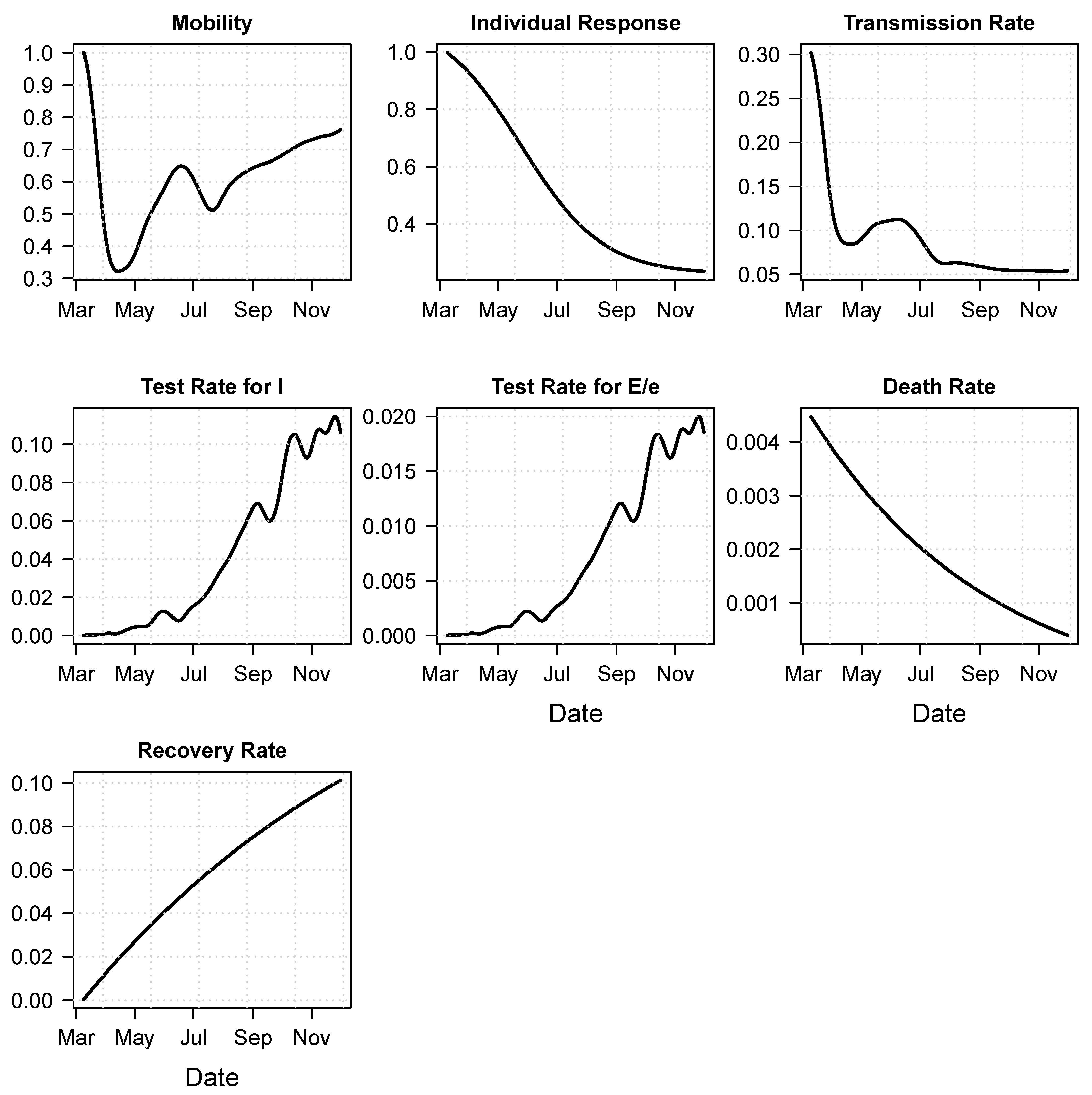
3.1. Calibration Results and Retrospective Analysis

The posterior means and $95\%$ credible intervals of the unknown parameters from the calibrated models are summarized in

Table 2. The posterior mean, the associated 95% credible intervals, and the corresponding prior support for the unknown parameters.

State/Parameters	q	${\mathit{\beta }}_0$	$\mathit{\kappa }$	${\mathit{x}}_1$	${\mathit{b}}_1$
Maharashtra	0.7314	0.3740	0.0215	95	0.1
	[0.6116, 0.8517]	[0.3125, 0.4355]	[0.0171, 0.0239]	[79.3739, 110.6261]	[0.1172, 0.163]
Karnataka	0.6865	0.3026	0.0235	77	0.2242
	[0.5756, 0.7995]	[0.2528, 0.3524]	[0.0196, 0.0274]	[64.3346, 89.6654]	[0.1873, 0.2611]
Andhra Pradesh	0.6988	0.2711	0.0112	70	0.2235
	[0.5853, 0.8138]	[0.2265, 0.3157]	[0.0094, 0.013]	[58.486, 81.514]	[0.1867, 0.2603]
Kerala	0.6924	0.1839	0.0104	69	0.2223
	[0.5802, 0.8064]	[0.1537, 0.2141]	[0.0087, 0.0121]	[57.6505, 80.3495]	[0.1857, 0.2589]
West Bengal	0.6883	0.4723	0.0647	41	0.1575
	[0.577, 0.8016]	[0.3946, 0.55]	[0.0541, 0.0753]	[34.2561, 47.7439]	[0.1316, 0.1834]
Prior support	[0.5, 1]	[0.1, 2]	[0.001, 1]	[1, 150]	[0.1, 0.5]
State/Parameters	$\mathbf{1}/{\mathbf{\mu }}_{\mathbf{E}}$	$\mathbf{1}/\mathbf{\alpha }$	${\mathit{k}}_{\mathit{I}}$	c
Maharashtra	21	7	39	0.4243
	[17.5458, 24.4542]	[5.8486, 8.1514]	[32.5851, 45.4149]	[0.3545, 0.4941]
Karnataka	23	6	70	0.17442
	[19.2166, 26.7778]	[5.0131, 6.9869]	[58.486, 81.514]	[0.1457, 0.2031]
Andhra Pradesh	21	6.5	69	0.4974
	[17.5458, 24.4542]	[5.4308, 7.5692]	[57.6505, 80.3495]	[0.4156, 0.5792]
Kerala	17	5	10	0.3903
	[14.207, 19.7964]	[4.5953, 6.4047]	[10.0627, 11.96]	[0.3261, 0.4545]
West Bengal	19	5.5	71	0.4505
	[15.875, 22.1252]	[4.1776, 5.8224]	[59.3215, 82.6785]	[0.3764, 0.5246]
Prior support	[11, 31]	[2, 14]	[10, 200]	[0.001, 1]

. The posterior means and 95% credible intervals of daily new tested positive cases, recoveries, and deaths of the calibrated SEIR models are shown in Figure 2 for the state of Karnataka. The corresponding posterior predictive mean for different infection stages and other time-dependent parameters are shown in Figure 3 and Figure 4 respectively. The posterior means and 95% credible intervals of daily new tested positive cases, recoveries, and deaths of the calibrated SEIR models for other states are shown in Figure 5. The 95% credible intervals contain the observed training and validation data for all the cases. This shows that the fitted model can explain the disease dynamics very well and it is also able to predict short-term disease progression.

The posterior means of the undetected infected proportion in Maharashtra, Karnataka, Andhra Pradesh, Kerala, and West Bengal are 46%, 49%, 48%, 43%, 52%, respectively. This indicates that the number of daily reported cases did not reflect the actual infected population, which might mislead decision-makers of the public health authorities and the public awareness and related preventive measures. The initial transmission rate ${\beta }_0$ is the biological transmission rate times the frequency of contact. ${\beta }_0$ for West Bengal is almost twice that of other states. Since the biological transmission rate should be the same, the average contact rate in West Bengal can be assumed to be twice that of other states. One possible reason for this could be the highest population density of West Bengal among these five states. The 95% credible interval for incubation periods $1/\alpha$ is 5–7 days for all states, which is similar to what has been reported in [29].

The posterior mean for the proportions of the asymptomatic and symptomatic cases for all five states are all around 30%. The posterior mean of the odd ratio $k_I$’s is around 70 for most of the states, which indicates that the symptomatic population has a much higher chance to be tested than the general public. However, we observed that the odd ratio $k_I$ for Kerala is around seven times lower than the average, which reflects the fact that the general public without any symptoms in Kerala has a much higher chance of being tested than in other states. This implies that the reported infected cases in Kerala reflect the actual infected cases more reliably. The 95% CI for the testing odd ratios of pre-symptomatic $E\left(e\right)$ against a random individual are ($24.5$, $38.5$), which are still quite high. The result is consistent with other reports stating that all the states have some contact tracing policies, and Kerala is one of the states which implemented a good testing policy at the very early stage of the pandemic.

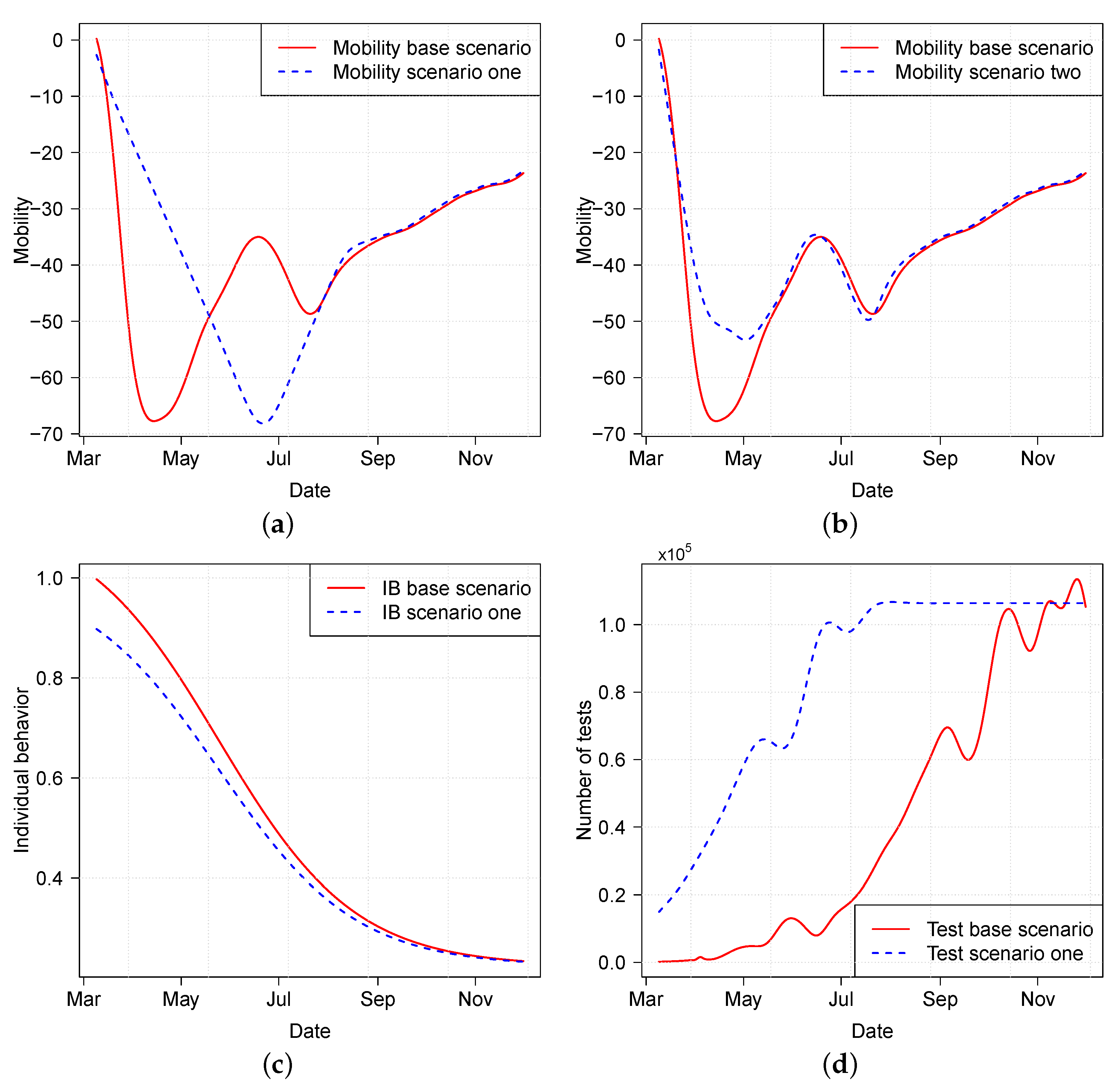
3.2. Effect of Various Intervention Policies

We use the calibrated model for Karnataka as an example to study the effect of various possible government intervention policies, especially in terms of lockdown, testing, and tracing. The calibrated state variables and time-dependent parameters of the SEIR model for Karnataka are displayed in Figure 3 and Figure 4. We consider the combinations of two possible initial lockdown strategies, one possible public awareness and personal behavior scenario, and one possible testing strategy, and their effects on the pandemic using the calibrated SEIR model.

The two proposed lockdown strategies are both less strict than the complete shutdown policy implemented by the government. The idea of the first one is to make the initial lockdown process a gradual one, very similar to the reverse of how the lockdown was lifted gradually during May and June 2020. We fit a linear regression for the mobility data from 20 April to 15 June 2020, and the negative of the fitted slope is used to construct the possible mobility function from 10 March to 20 April 2021. The second initial lockdown scenario is about implementing a sudden lockdown but with fewer restrictions, which would translate to a higher minimum mobility level than the value from the observed mobility data. The blue dash curves in Figure 6a,b show the mobility function for lock-down scenarios one and two respectively. For the individual behavior factor function $p\left(t\right)$, we considered a scenario where the initial response is 90% of the base scenario, which represents the public awareness based on the concurrent situations in other countries. The blue dash curve in Figure 6c shows the possible individual behavior function. An exponential acceleration of the reported positive cases started from the time around 1 July 2021, which might be due to the increase in testing during the same period. From Figure 7, our model indicates that the actual outbreak may have already started around 1 May 2021, and the actual infected cases are much higher than the reported data before 1 July 2021. Our hypothetical testing scenario shifts the testing trend that is observed from 1 July to the beginning of the pandemic and then maintains a constant test level from August. Figure 6d plot the hypothetical daily tests, which represent a better intervention strategy in terms of testing and tracking.

Results of different combinations of the proposed intervention strategies are shown in Figure 8, and

Table 3. Summaries of outcomes for different intervention strategies.

Scenarios	Cumulative Infected	Cumulative Death	Peak Infected	Peak Death
M0PB0T0	883,632	11,219	10,037	138
M1PB0T0	7,033,837	127,646	90,784	1505
M1PB0T1	1,307,246	42,159	19,911	644
M1PB1T0	1,077,677	15,627	11,445	162
M1PB1T1	110,325	3901	1702	59
M2PB0T0	5,163,521	73,859	67,834	989
M2PB0T1	338,997	7731	4035	101
M2PB1T0	558,504	7277	6163	87
M2PB1T1	27,777	728	335	9

. The posterior predictive mean of the outbreak size and outbreak peak both in terms of death and infected cases are shown in this table. We used the following notations to represent different combinations of these intervention factors. $Mi$, $i=0,1,2$ represents lockdown scenario i, $PBi$, $i=0,1$ represents the public behavior scenario i, and $Ti$, $i=0,1$ represents the testing scenario i. Here $i=0$ represents the base case, i.e., the true observed data for each of these factors. $MiPBjTk$ represents the scenario which is the combination of $Mi$, $PBj$, and $Tk$. As expected, both of the proposed lockdown strategies result in higher expected cumulative infected cases and peak infected cases when the individual behavior and the testing strategies remain the same at the base level. However, the improved testing strategy reduces the cumulative deaths, peak deaths, cumulative cases, and peak cases significantly even with both proposed lockdown strategies. The effect of the second initial lockdown strategy is significantly better for both cumulative and peak cases and deaths than the first one when the public behavior and the testing scenarios are held constant. It is also observed that implementing the new testing strategy with the baseline $p\left(t\right)$ has a higher impact on the mitigation than considering the new $p\left(t\right)$ with baseline testing. Our study suggests that if better public awareness, individual response, and testing strategies are implemented, then the number of deaths could be dramatically reduced from 11,219 to below one thousand, even with the proposed relaxed lockdown policies. Similarly, the cumulative infected cases can be reduced from 883,632 to 27,777 and the peak daily positive cases can be reduced from 10,037 to a few hundred. This would help in reducing the burden on the healthcare system significantly. A less restrictive lockdown with better public awareness and an improved testing strategy would not only help in mitigating the disease substantially but could also avoid the tremendous personal agony, job loss, deaths, etc., that migrant workers suffered due to the original sudden and strict lockdown.

In conclusion, to relieve stress for migration workers, a less strict initial lockdown could have been implemented. At the same time, in order to control the disease outbreak size, it is critical to educate the public on the importance of individual prevention measures such as social distancing, wearing masks and personal hygiene, and symptomatic self-quarantine. If the vast majority of people can cooperate with government policies, maintain a certain social distance, and wear face masks, the transmission rate $\beta \left(t\right)$ will be reduced. Our study also indicates that establishing convenient and adequate testing as early as possible is the most crucial intervention strategy in mitigating the disease.

4. Discussion and Conclusions

We propose a population-based modified SEIR compartmental model to conduct a retrospective analysis of the effects of government policies regarding lockdown, testing, individual protective actions, and screening strategies on the transmission of COVID-19 in India during the period of mid-March to early December 2020. It is to be noted that much simpler parametric models such as exponential and Gompertz growth models are also good alternatives to SEIR models for infectious disease modeling and are generally used for short-term prediction [30,31]. However, these methods do not explicitly consider the lockdown, personal behavior, testing, and quarantining effect in the model. So, it is difficult to conduct a retrospective analysis of these interventions using such models. Our modified SEIR model takes into account two different pathways, viz. $S\to E\to I\to R$ and $s\to e\to r$ for disease progression. We also consider a variable time-dependent disease-transmission rate based on the mobility data and a personal behavioral function. The testing data are used in determining the transition rate from asymptomatic and symptomatic states to the tested positive state. To ensure the efficiency of the healthcare system over time, the death and recovery rates are also considered to be time-varying functions. This novel approach of including all these factors together in the SEIR model facilitates the retrospective analysis of different types of intervention policies, viz., less extreme shutdown policies, new testing and contact tracing policies, and personal behavioral effects. We also use a Bayesian inferential method to calibrate the model to the reported data on daily infected cases, daily death cases, and daily recovered cases. A non-Bayesian approach provides only the best possible estimates of the parameters and an optimal prediction for disease progression. On the other hand, the Bayesian method also provides uncertainties in the estimates and predictions. The uncertainties in the model were expressed as a posterior probability distribution of model parameters, which provides additional valuable insights for healthcare decision-makers.

A retrospective analysis was carried out using the calibrated SEIR model for five representative Indian states. The calibrated model is used to estimate the undetected infected cases in each of these states, and shows that the actual outbreak started much earlier than implied by the publicly reported data on infection. Using the calibrated model, we study a few alternative lockdown strategies other than the original sudden strict lockdown which can reduce the humanitarian crisis for millions of migrant workers. The study suggests that the strict practice of individual protective actions such as social distancing, mask-wearing, self-quarantine, and adequate early testing is critical to incorporate a much moderate initial lockdown policy and simultaneously mitigate the disease progression. Therefore, it is recommended that during the onset of such infectious diseases, the government should focus on increasing testing rates, contact tracing, and public awareness along with less severe and gradual shutdown policies. These alternative intervention strategies could potentially avoid the tremendous economic, physical, and social stress for all the citizens and the humanitarian crisis faced by migrant workers and laborers.

It is to be noted that medical intervention strategies such as vaccinations and drug therapies are not considered in our model as they were not available at the time period considered. Our SEIR model can be extended to incorporate these medical intervention effects, especially for the later period (e.g., the second and the third wave) of the disease progression. This is one of our future research goals.

References

1. WHO. Director-General Opening Remarks at the Media Briefing on COVID-19—13 March 2020. Available online: https://www.who.int/director-general/speeches/detail/who-director-general-s-opening-remarks-at-the-mission-briefing-on-covid-19 (accessed on 18 March 2020).
2. Flaxman, S.; Mishra, S.; Gandy, A.; Unwin, H.J.T.; Mellan, T.A.; Coupland, H.; Whittaker, C.; Zhu, H.; Berah, T.; Eaton, J.W.; et al. Estimating the effects of non-pharmaceutical interventions on COVID-19 in Europe. Nature 2020, 584, 257–261. [Google Scholar] [CrossRef] [PubMed]
3. Pai, C.; Bhaskar, A.; Rawoot, V. Investigating the dynamics of COVID-19 pandemic in India under lockdown. Chaos Solitons Fractals 2020, 138, 109988. [Google Scholar] [CrossRef] [PubMed]
4. Hellewell, J.; Abbott, S.; Gimma, A.; Bosse, N.I.; Jarvis, C.I.; Russell, T.W.; Munday, J.D.; Kucharski, A.J.; Edmunds, W.J.; Sun, F.; et al. Feasibility of controlling COVID-19 outbreaks by isolation of cases and contacts. Lancet Glob. Health 2020, 8, e488–e496. [Google Scholar] [CrossRef] [Green Version]
5. Ali, S.T.; Wang, L.; Lau, E.H.; Xu, X.K.; Du, Z.; Wu, Y.; Leung, G.M.; Cowling, B.J. Serial interval of SARS-CoV-2 was shortened over time by nonpharmaceutical interventions. Science 2020, 369, 1106–1109. [Google Scholar] [CrossRef]
6. Chu, D.K.; Akl, E.A.; Duda, S.; Solo, K.; Yaacoub, S.; Schünemann, H.J.; El-harakeh, A.; Bognanni, A.; Lotfi, T.; Loeb, M.; et al. Physical distancing, face masks, and eye protection to prevent person-to-person transmission of SARS-CoV-2 and COVID-19: A systematic review and meta-analysis. Lancet 2020, 395, 1973–1987. [Google Scholar] [CrossRef]
7. Huang, Q.; Mondal, A.; Jiang, X.; Horn, M.A.; Fan, F.; Fu, P.; Wang, X.; Zhao, H.; Ndeffo-Mbah, M.; Gurarie, D. SARS-CoV-2 transmission and control in a hospital setting: An individual-based modelling study. R. Soc. Open Sci. 2021, 8, 201895. [Google Scholar] [CrossRef]
8. Chiu, W.A.; Fischer, R.; Ndeffo-Mbah, M.L. State-level needs for social distancing and contact tracing to contain COVID-19 in the United States. Nat. Hum. Behav. 2020, 4, 1080–1090. [Google Scholar] [CrossRef]
9. Godio, A.; Pace, F.; Vergnano, A. SEIR modeling of the Italian epidemic of SARS-CoV-2 using computational swarm intelligence. Int. J. Environ. Res. Public Health 2020, 17, 3535. [Google Scholar] [CrossRef]
10. Picchiotti, N.; Salvioli, M.; Zanardini, E.; Missale, F. COVID-19 pandemic: A mobility-dependent SEIR model with undetected cases in Italy, Europe and US. arXiv 2020, arXiv:2005.08882. [Google Scholar]
11. Chu, I.Y.H.; Alam, P.; Larson, H.J.; Lin, L. Social consequences of mass quarantine during epidemics: A systematic review with implications for the COVID-19 response. J. Travel Med. 2020, 27, taaa192. [Google Scholar] [CrossRef]
12. Joshi, A. COVID-19 pandemic in India: Through psycho-social lens. J. Soc. Econ. Dev. 2021, 23, 414–437. [Google Scholar] [CrossRef] [PubMed]
13. Soni, P. Effects of COVID-19 lockdown phases in India: An atmospheric perspective. Environ. Dev. Sustain. 2021, 23, 12044–12055. [Google Scholar] [CrossRef] [PubMed]
14. Saikia, D.; Bora, K.; Bora, M.P. COVID-19 outbreak in India: An SEIR model-based analysis. Nonlinear Dyn. 2021, 104, 4727–4751. [Google Scholar] [CrossRef] [PubMed]
15. Sarkar, K.; Khajanchi, S.; Nieto, J.J. Modeling and forecasting the COVID-19 pandemic in India. Chaos Solitons Fractals 2020, 139, 110049. [Google Scholar] [CrossRef]
16. Malavika, B.; Marimuthu, S.; Joy, M.; Nadaraj, A.; Asirvatham, E.S.; Jeyaseelan, L. Forecasting COVID-19 epidemic in India and high incidence states using SIR and logistic growth models. Clin. Epidemiol. Glob. Health 2021, 9, 26–33. [Google Scholar] [CrossRef]
17. Singh, B.C.; Alom, Z.; Hu, H.; Rahman, M.M.; Baowaly, M.K.; Aung, Z.; Azim, M.A.; Moni, M.A. COVID-19 Pandemic Outbreak in the Subcontinent: A Data Driven Analysis. J. Pers. Med. 2021, 11, 889. [Google Scholar] [CrossRef]
18. Al-Raeei, M.; El-Daher, M.S.; Solieva, O. Applying SEIR model without vaccination for COVID-19 in case of the United States, Russia, the United Kingdom, Brazil, France, and India. Epidemiol. Methods 2021, 10, 20200036. [Google Scholar] [CrossRef]
19. Poonia, R.C.; Saudagar, A.K.J.; Altameem, A.; Alkhathami, M.; Khan, M.B.; Hasanat, M.H.A. An Enhanced SEIR Model for Prediction of COVID-19 with Vaccination Effect. Life 2022, 12, 647. [Google Scholar] [CrossRef]
20. Calvetti, D.; Hoover, A.; Rose, J.; Somersalo, E. Bayesian dynamical estimation of the parameters of an SE(A)IR COVID-19 spread model. arXiv 2020, arXiv:2005.04365. [Google Scholar]
21. Gelman, A.; Carlin, J.B.; Stern, H.S.; Rubin, D.B. Bayesian Data Analysis, 2nd ed.; Chapman and Hall/CRC: Boca Raton, FL, USA, 2004. [Google Scholar]
22. Mahajan, A.; Solanki, R.; Sivadas, N. Estimation of undetected symptomatic and asymptomatic cases of COVID-19 infection and prediction of its spread in the USA. J. Med. Virol. 2021, 93, 3202–3210. [Google Scholar] [CrossRef]
23. COVID-19 Community Mobility Reports. Available online: https://www.google.com/covid19/mobility/ (accessed on 20 January 2021).
24. India COVID-19 Tracker. 2020. Available online: https://www.covid19india.org/ (accessed on 20 January 2021).
25. Haario, H.; Saksman, E.; Tamminen, J. An adaptive Metropolis algorithm. Bernoulli 2001, 7, 223–242. [Google Scholar] [CrossRef] [Green Version]
26. Gelman, A.; Rubin, D.B. Inference from iterative simulation using multiple sequences. Stat. Sci. 1992, 7, 457–472. [Google Scholar] [CrossRef]
27. R Core Team. R: A Language and Environment for Statistical Computing; R Foundation for Statistical Computing: Vienna, Austria, 2020. [Google Scholar]
28. Soetaert, K.; Petzoldt, T.; Setzer, R.W. Solving Differential Equations in R: Package deSolve. J. Stat. Softw. 2010, 33, 1–25. [Google Scholar] [CrossRef]
29. Lauer, S.A.; Grantz, K.H.; Bi, Q.; Jones, F.K.; Zheng, Q.; Meredith, H.R.; Azman, A.S.; Reich, N.G.; Lessler, J. The incubation period of coronavirus disease 2019 (COVID-19) from publicly reported confirmed cases: Estimation and application. Ann. Intern. Med. 2020, 172, 577–582. [Google Scholar] [CrossRef] [PubMed] [Green Version]
30. Bartolomeo, N.; Trerotoli, P.; Serio, G. Short-term forecast in the early stage of the COVID-19 outbreak in Italy. Application of a weighted and cumulative average daily growth rate to an exponential decay model. Infect. Dis. Model. 2021, 6, 212–221. [Google Scholar] [CrossRef]
31. Pelinovsky, E.; Kokoulina, M.; Epifanova, A.; Kurkin, A.; Kurkina, O.; Tang, M.; Macau, E.; Kirillin, M. Gompertz model in COVID-19 spreading simulation. Chaos Solitons Fractals 2022, 154, 111699. [Google Scholar] [CrossRef]
Figure 1. COVID-19 transmission flow diagram.
Mathematics 10 04037 g001
Figure 2. The posterior mean and 95% credible bands for reported tested positive cases, death, and recovery cases of state Karnataka. The blue circles represent the observed data, the red lines represent the posterior mean and the red bands represent the 95% credible interval. The vertical dashed black lines divide the training and validation dataset.
Mathematics 10 04037 g002
Figure 3. The posterior predictive mean of different infection stages from the SEIR model for Karnataka.
Mathematics 10 04037 g003
Figure 4. The posterior mean of the time-dependent parameters from the SEIR model for Karnataka.
Mathematics 10 04037 g004
Figure 5. The posterior mean and 95% credible bands for reported cases, death, and recovery cases of other states. The blue circles represent the observed data, the red lines represent the posterior mean and the red bands represent the 95% credible interval. The vertical dashed black lines divide the training and validation dataset.
Mathematics 10 04037 g005
Figure 6. (a) Less strict lockdown scenario one; (b) Less strict lockdown scenario two. (c) Individual behavior scenario one; (d) Testing scenario one.
Mathematics 10 04037 g006
Figure 7. Fitted posterior predictive mean for Karnataka.
Mathematics 10 04037 g007
Figure 8. The posterior predictive mean for the various intervention scenarios for Karnataka.
Mathematics 10 04037 g008