Inverse Problem for the Integral Dynamic Models with Discontinuous Kernels

Abstract

The objective of this paper was to present a new inverse problem statement and numerical method for the Volterra integral equations with piecewise continuous kernels. For such Volterra integral equations of the first kind, it is assumed that kernel discontinuity curves are the desired ones, but the rest of the information is known. The resulting integral equation is nonlinear with respect to discontinuity curves which correspond to integration bounds. A direct method of discretization with a posteriori verification of calculations is proposed. The family of quadrature rules is employed for approximation purposes. It is shown that the arithmetic complexity of the proposed numerical method is $\mathcal{O}\left(N^3\right)$. The method has first-order convergence. A generalization of the method is also proposed for the case of an arbitrary number of discontinuity curves. The illustrative examples are included to demonstrate the efficiency and accuracy of proposed solver.

1. Introduction

The paper deals with the numerical study of integral dynamic models based on Volterra integral equations of the first kind with kernels having discontinuities on a set of smooth curves. Namely, let us consider the following linear integral model

$${\int }_0^{t}K(t,s)x\left(s\right)ds=f\left(t\right),0\le s\le t\le T,f\left(0\right)=0,$$

(1)

where the kernel $K(t,s)$ is defined as follows

$$K(t,s)=\left\{\begin{array}{c}{K}_1(t,s),t,s\in m_1,\hfill \\ \cdots \cdots \cdots \cdots \hfill \\ K_n(t,s),t,s\in m_n.\hfill \end{array}\right.$$

(2)

where $m_i=\{t,s|{\alpha }_{i-1}\left(t\right)<s<{\alpha }_i\left(t\right)\}$, ${\alpha }_0\left(t\right)=0,{\alpha }_n\left(t\right)=t,i=\overline{1,n},$ ${\alpha }_i\left(t\right),$$f\left(t\right)\in {\mathcal{C}}_{[0,T]}^1,$ functions $K_i(t,s)$ have continuous derivatives with respect to t for $(t,s)\in cl\left(m_i\right),$$K_n(t,t)\ne 0,$${\alpha }_i\left(0\right)=0$, $0<{\alpha }_1\left(t\right)<{\alpha }_2\left(t\right)<$⋯$<{\alpha }_{n-1}\left(t\right)<t$, for $t\in (0,T]$, functions ${\alpha }_1\left(t\right),\cdots ,{\alpha }_{n-1}\left(t\right)$ increase in a small neighborhood $0\le t\le \tau ,$ $0<{\alpha }_1^{\prime }\left(0\right)\le$⋯$\le {\alpha }_{n-1}^{\prime }\left(0\right)<1,$ and $cl\left(m_i\right)$ denotes closure of set $m_i$.

Such weakly regular Volterra equations of the first kind with piecewise continuous kernels were first classified and employed by Sidorov [1] and Lorenzi [2] and extensively studied by many authors during the last decade. Here, readers may refer to the monograph by Sidorov [3] and references therein. Volterra operator equations of the first kind were studied by Sidorov and Sidorov [4], who obtained the sufficient conditions for the existence of a unique solution. Muftahov, Tynda and Sidorov [5] employed direct quadrature methods for the solution of such equations in both linear and nonlinear cases. Such Volterra models have many applications in modeling evolving dynamical processes including energy storage systems [6,7] and models for the electric power systems development [8]. The nonlinear integral equations with unknown lower limits of integration are in the core of different models in economics, operations research, population biology, and environmental sciences. The systems of such equations and the existence and uniqueness theorems studied by Hritonenko and Yatsenko [9,10]. For a comprehensive introduction to numerical methods for the solution to the Volterra equations of the first kind (including cases of variable integration limits), we refer the reader to books by Brunner [11] and Apartsyn [12].

Inverse Problem

The classical problem statement for model (1) and (2) is to determine function $x\left(t\right)$ under the assumption of a known kernel $K(t,s)$ and source function $f\left(t\right)$. However, a number of applications of model (1) and (2) in practice leads to the inverse problem of determining the curves ${\alpha }_i\left(t\right)$. With this formulation, the Equation (1) is interpreted as a nonlinear integral equation with unknown integration limits, its numerical study is a novel, mathematically challenging problem. The theory of such equations has not yet been developed and attacked for the first time in the present paper.

Indeed, if one considers just single term ($i=2$, $K_2(t,s)\equiv 0$) of Equation (1) as an integral operator

$$\mathcal{A}\left({\alpha }_1\left(t\right)\right):={\int }_0^{{\alpha }_1\left(t\right)}K(t,s)x\left(s\right)ds,$$

it can be outlined that such an operator is obviously nonlinear since it is not homogeneous nor additive.

The complexity of the discretization is primarily related to the approximation of integrals with unknown lengths of integration segments.

The models described by integral equations with unknown integration limits were first formulated in the seminal works of Glushkov. Here, readers may refer to his book [13]. The applications of such integral models in economics were investigated in the works of Hritonenko and Yatsenko, as can be seen, for example, in ref. [14] and book [15]. The number of direct and iterative numerical methods are proposed by Tynda, and here readers may refer to [16,17,18].

The objective of this paper is to provide the new problem statement (inverse problem) as well as to propose the efficient numerical method for the solution. In this paper, the direct method of discretization with a posteriori verification of calculations is proposed for the inverse problem (1) and (2) in the case of $n=2$.

The paper is organized as follows. Section 3 analyzes the arithmetic complexity of calculations. A generalization of the method is also proposed in Section 4 for an arbitrary number of discontinuity curves. In Section 5, the numerical results of solving model problems are given.

2. Numerical Method

Let us first consider in detail the problem (1)–(2) for $n=2$, which consists in determining the unknown function ${\alpha }_1\left(t\right)=\alpha \left(t\right)$:

$$\underset{0}{\overset{\alpha \left(t\right)}{\int }}{K}_1(t,s)x\left(s\right)ds+\underset{\alpha \left(t\right)}{\overset{t}{\int }}{K}_2(t,s)x\left(s\right)ds=f\left(t\right),t\in [0,T].$$

(3)

In order to construct an approximate solution, we introduce a grid of nodes (not necessarily uniform) on the segment $[0,T]$:

$$0=t_0<t_1<\cdots <t_N=T.$$

Let the approximate solution ${\alpha }_N\left(t\right)$ be a piecewise linear function constructed on the points

$$(t_k,{\alpha }_k),{\alpha }_k=\alpha \left(t_k\right),k=0,1,2,\dots ,N.$$

Let us start defining the unknown values ${\alpha }_k,k=0,1,2,\dots ,N$. In order to carry out the discretization of the Equation (3), we also introduce an auxiliary integer-valued function

$$v\left(k\right)=v_k\mathrm{if}{t}_{v_k-1}<{\alpha }_k⩽t_{v_k},k=1,2,\dots ,N.$$

In other words, $v\left(k\right)$ denotes the number of the grid segment that the unknown value ${\alpha }_k$ falls on. Since $\alpha \left(t\right)$ is a monotonically increasing function and $\alpha \left(t\right)<t$, we have

$$v_k⩽k\mathrm{and}{v}_p⩽v_m\mathrm{for}p<m.$$

We require that, at the nodes of the grid $t=t_k,k=1,2,\dots ,N$, the Equation (3) turn:

$$\underset{0}{\overset{{\alpha }_k}{\int }}{K}_1(t_k,s)x\left(s\right)ds+\underset{{\alpha }_k}{\overset{t}{\int }}{K}_2(t_k,s)x\left(s\right)ds=f\left(t_k\right),k=1,2,\dots ,N.$$

(4)

Using the definition of $v_k$ and denoting $f_k=f\left(t_k\right)$, we can represent the Equation (4) in the following form

$$\begin{array}{cc}\hfill \sum _{m=1}^{v_k-1}\underset{t_{m-1}}{\overset{t_m}{\int }}{K}_1(t_k,s)x\left(s\right)ds+\underset{t_{v_k-1}}{\overset{{\alpha }_k}{\int }}{K}_1(t_k,s)x\left(s\right)ds& \\ \hfill +\underset{{\alpha }_k}{\overset{t_{v_k}}{\int }}{K}_2(t_k,s)x\left(s\right)ds+\sum _{p=v_k}^{k-1}\underset{t_p}{\overset{t_{p+1}}{\int }}{K}_2(t_k,s)x\left(s\right)ds=f_k.\end{array}$$

(5)

Assuming that the values $v_k,k=1,2,\dots ,N,$ are somehow obtained, we approximate the integrals in (5) as follows

$$\begin{array}{cc}\hfill \sum _{m=1}^{v_k-1}{K}_1\left(t_k,\frac{t_{m-1}+t_m}{2}\right)x\left(\frac{t_{m-1}+t_m}{2}\right)(t_m-t_{m-1})+({\alpha }_k-t_{v_k-1})K_1(t_k,t_{v_k-1})x\left(t_{v_k-1}\right)& \\ \hfill +(t_{v_k}-{\alpha }_k)K_2(t_k,t_{v_k})x\left(t_{v_k}\right)+\sum _{p=v_k}^{k-1}{K}_2\left(t_k,\frac{t_p+t_{p+1}}{2}\right)x\left(\frac{t_p+t_{p+1}}{2}\right)(t_{p+1}-t_p)=f_k.\end{array}$$

(6)

Here, to approximate the integrals in the first and fourth terms of (5), the quadrature rule of the middle rectangles is applied. For the second and third terms, the formulas of the left and right rectangles are applied, respectively.

From (6), we have

$${\alpha }_k=\frac{f_k-S_1-S_2+t_{v_k-1}{K}_1(t_k,t_{v_k-1})x\left(t_{v_k-1}\right)-t_{v_k}{K}_2(t_k,t_{v_k})x\left(t_{v_k}\right)}{K_1(t_k,t_{v_k-1})x\left(t_{v_k-1}\right)-K_2(t_k,t_{v_k})x\left(t_{v_k}\right)},$$

(7)

where

$$S_1=\sum _{m=1}^{v_k-1}{K}_1\left(t_k,\frac{t_{m-1}+t_m}{2}\right)x\left(\frac{t_{m-1}+t_m}{2}\right)(t_m-t_{m-1}),$$

$$S_2=\sum _{p=v_k}^{k-1}{K}_2\left(t_k,\frac{t_p+t_{p+1}}{2}\right)x\left(\frac{t_p+t_{p+1}}{2}\right)(t_{p+1}-t_p).$$

Thus, with the knowledge of the numbers $v_k,k=\overline{1,N},$ approximate values ${\alpha }_k$ of the unknown function at grid points can be found by the explicit Formula (7).

The idea of determining the numbers $v_k$ consists of sequentially iterating over the possible values $v_k$ for each node number $k=1,2,\dots ,N$:

$$v_1=1;$$

$$v_2=v_1\mathrm{or}{v}_2=2;$$

$$v_3=v_2\mathrm{or}{v}_3=v_2+1\mathrm{or}{v}_3=3;$$

$$·······························$$

$$v_k=v_{k-1},v_k=v_{k-1}+1,v_k=v_{k-1}+2,\dots ,v_k=k.$$

For each possible $v_k$, the corresponding values ${\alpha }_k$ are calculated using the Formula (7). The iteration for each value k stops if the condition ${\alpha }_k\in (t_{v_k-1},t_{v_k}]$ is met, confirming the assumption that ${\alpha }_k$ belongs to the specified interval.

It is easy to see that the estimate of the accuracy of the approximate solution for the problem (3) according to the proposed computational scheme as follows

$$\underset{t\in [0,T]}{max}|{\alpha }_N\left(t\right)-\alpha \left(t\right)|=\mathcal{O}\left(\frac{1}{N}\right),$$

(8)

meaning that the proposed method has the first order of convergence. As a note, let us highlight here that for the introduction to the theory of uniform approximation of the functions by polynomials, readers may refer to the book by Dziadyk [19], and for the theory of functional equations and applications of functional analysis to applied analysis and computational mathematics, readers may refer to the classic book by Kantorovich and Akilov [20].

3. Arithmetic Complexity

Let us turn to the question of the computational cost of the proposed method from the point of view of the arithmetic complexity of calculations. We will count the number of required arithmetic operations, calculations of the values of the functions included in the equation, as well as operations for comparing the two numbers.

• Calculation of the values of functions $f\left(t\right),K_1(t,s),K_2(t,s)$ and $x\left(t\right)$ at grid nodes and at midpoints:

  $$4N+N^2;$$
• Calculation of the values ${\alpha }_k,k=1,2,\dots ,N$:

  $$12·\stackrel{\mathrm{summation}{S}_1,S_2}{\overbrace{3·\sum _{k=1}^{N}2·\frac{1+k-1}{2}(k-1)}}=36\sum _{k=1}^{N}k(k-1)$$

  $$=36\left(\frac{N(N+1)(2N+1)}{6}-\frac{1+N}{2}N\right)=12N(N^2-1);$$
• Estimation of the number of arithmetic operations $P_N^1$ to iterate over possible values ${\alpha }_k$:

  $$P_N^1⩽\sum _{k=1}^N\left(1+2+\cdots +k\right)=\frac{1}{2}\sum _{k=1}^{N}k(k+1)=\frac{N(N+1)(N+2)}{6};$$
• Estimation of the number of comparison operations $P_N^2$ when iterating over possible values ${\alpha }_k$:

  $$P_N^2⩽2P_N^1=\frac{N(N+1)(N+2)}{3}.$$

Thus, we obtain a general estimate $P\left(N\right)$ of the arithmetic complexity of the method:

$$\begin{array}{c}\hfill P\left(N\right)=4N+N^2+12N(N^2-1)+P_N^1+P_N^2⩽4N+N^2\\ \hfill +12N(N^2-1)+\frac{N(N+1)(N+2)}{6}\\ \hfill +\frac{N(N+1)(N+2)}{3}=\frac{N(25N^2+5N-14)}{2}=\mathcal{O}\left(N^3\right).\end{array}$$

(9)

4. General Case

The presented approach is naturally generalized to the case of a system of integral equations with an arbitrary number of discontinuity curves ${\alpha }_i\left(t\right)$.

Let us consider the problem of determining the entire family of discontinuity curves

$${\alpha }_1\left(t\right),{\alpha }_2\left(t\right),\dots ,{\alpha }_{n-1}\left(t\right),$$

of the following nonlinear integral model

$$\left\{\begin{array}{c}{\displaystyle \sum _{i=1}^n}\underset{{\alpha }_{i-1}\left(t\right)}{\overset{{\alpha }_i\left(t\right)}{\int }}{K}_{1,i}(t,s,x_i\left(s\right))ds=f_1\left(t\right);\hfill \\ \cdots \cdots \cdots \cdots \cdots \cdots \cdots \cdots \cdots \cdots \cdots \cdots \cdots \cdots \cdots \hfill \\ {\displaystyle \sum _{i=1}^n}\underset{{\alpha }_{i-1}\left(t\right)}{\overset{{\alpha }_i\left(t\right)}{\int }}{K}_{n-1,i}(t,s,x_i\left(s\right))ds=f_{n-1}\left(t\right),t\in [0,T].\hfill \end{array}\right.$$

(10)

Here, ${\alpha }_0\left(t\right)=0,{\alpha }_n\left(t\right)=t$ and the functions ${\alpha }_i\left(t\right),i=\overline{1,n-1},$ satisfy the following conditions: ${\alpha }_i\left(t\right)\in {\mathcal{C}}_{[0,T]}^1,$${\alpha }_i\left(0\right)=0$, $0<{\alpha }_1\left(t\right)<{\alpha }_2\left(t\right)<$⋯$<{\alpha }_{n-1}\left(t\right)<t$, for $t\in (0,T]$, functions ${\alpha }_1\left(t\right),\cdots ,{\alpha }_{n-1}\left(t\right)$ increase in a small neighborhood $0\le t\le \tau ,$ $0<{\alpha }_1^{\prime }\left(0\right)\le$⋯$\le {\alpha }_{n-1}^{\prime }\left(0\right)<1.$

In order to construct an approximate solution, let us introduce a grid of nodes on the segment $[0,T]$:

$$0=t_0<t_1<\cdots <t_N=T.$$

Let approximate solutions ${\alpha }_{i,N}\left(t\right)$ be piecewise linear functions constructed on the points

$$(t_k,{\alpha }_{i,k}),{\alpha }_{i,k}={\alpha }_i\left(t_k\right),i=1,2,\dots n-1,k=0,1,2,\dots ,N.$$

To discretize the system of Equation (10), we also introduce an auxiliary integer-valued vector function

$$\left\{v_i\left(k\right)\right\}=v_{i,k}\mathrm{if}{t}_{v_{i,k}-1}<{\alpha }_{i,k}⩽t_{v_{i,k}},i=1,2,\dots n-1,k=1,2,\dots ,N.$$

where $v_i\left(k\right)$ denotes the number of the grid segment on which the unknown value ${\alpha }_{i,k}$ falls. Since ${\alpha }_i\left(t\right)$ are monotonically increasing functions and ${\alpha }_i\left(t\right)<t$, we have

$$v_{i,k}⩽k\mathrm{and}{v}_{i,p}⩽v_{i,m}\mathrm{for}p<m,\forall i=\overline{1,n-1}.$$

Then, starting with sufficiently large values N, the system (10) in the nodes $t_k$ of the grid can be represented as follows

$$\begin{array}{c}\hfill \sum _{m=1}^{v_{1,k}-1}\underset{t_{m-1}}{\overset{t_m}{\int }}{K}_{i,1}(t_k,s,x_1\left(s\right))ds+\underset{t_{v_{1,k}-1}}{\overset{{\alpha }_{1,k}}{\int }}{K}_{i,1}(t_k,s,x_1\left(s\right))ds\\ \hfill +\underset{{\alpha }_{1,k}}{\overset{t_{v_{1,k}}}{\int }}{K}_{i,2}(t_k,s,x_2\left(s\right))ds+\cdots +\underset{t_{v_{n-1,k}-1}}{\overset{{\alpha }_{n-1,k}}{\int }}{K}_{i,n-1}(t_k,s,x_{n-1}\left(s\right))ds\\ \hfill +\underset{{\alpha }_{n-1,k}}{\overset{t_{v_{n-1,k}}}{\int }}{K}_{i,n}(t_k,s,x_n\left(s\right))ds+\sum _{p=v_{n-1,k}}^{k-1}\underset{t_p}{\overset{t_{p+1}}{\int }}{K}_{i,n}(t_k,s,x_n\left(s\right))ds=f_i\left(t_k\right),\end{array}$$

(11)

$$i=1,2,\dots ,n-1,k=1,2,\dots ,N.$$

Approximating the integrals in (11), as before in (6), we obtain a system of linear algebraic equations with respect to the coefficients ${\alpha }_{i,k}$.

Next, these systems of equations are successively solved for each of the permissible sets of values of $v_{i,k}$ and selection is performed according to a principle similar to the scalar case.

5. Numerical Experiments

Let us illustrate the effectiveness of the proposed algorithm by the example of solving two model problems.

5.1. Problem 1

Let us consider the following equation

$$\underset{0}{\overset{\alpha \left(t\right)}{\int }}{(t-s)}^2{e}^{s}ds+\underset{\alpha \left(t\right)}{\overset{t}{\int }}(t+s)e^{s}ds=e^{\frac{2}{3}{t}^2}\left(\frac{4}{9}{t}^4-\frac{4}{3}{t}^3-t^2+1\right)+e^t(2t-1)-t^2-2t-2,$$

(12)

The exact solution of this problem is the function $\alpha \left(t\right)=\frac{2}{3}{t}^2$, $t\in [0,1]$.

The results of solving Equation (12) are given in

Table 1. The dependence of the error on the number of grid nodes for Problem 1.

N	16	32	64	128	256	512	1024	2048	4096
${\epsilon }_N$	0.075	0.0094	0.00273	0.00079	$5.43\times {10}^{-5}$	$1.61\times {10}^{-5}$	$4.21\times {10}^{-6}$	$1.12\times {10}^{-6}$	$3.11\times {10}^{-7}$
r	—	2.99	1.78	1.79	3.86	1.75	1.93	1.91	1.85

, in which the following designations are adopted: N is the number of grid nodes, ${\epsilon }_N=\underset{t\in [0,T]}{max}|{\alpha }_N\left(t\right)-\alpha \left(t\right)|$ is the error norm, and $r={log}_2\left(\frac{{\epsilon }_N}{{\epsilon }_{2N}}\right)$ is the order of accuracy.

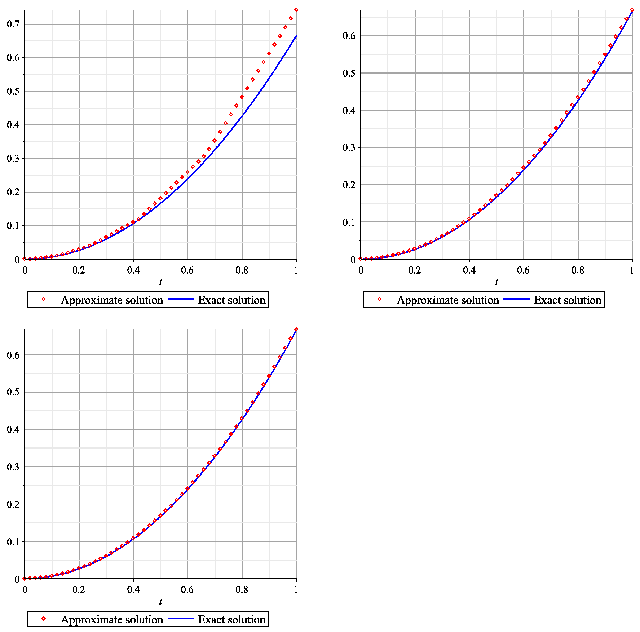
A graphical illustration of convergence is shown in Figure 1.

5.2. Problem 2

Let us consider the following equation

$$\underset{0}{\overset{\alpha \left(t\right)}{\int }}{(t-s)}^{2}x\left(s\right)ds+\underset{\alpha \left(t\right)}{\overset{t}{\int }}(t+s)x\left(s\right)ds=f\left(t\right),t\in [0,1.1],$$

(13)

where $x\left(t\right)=e^t$, and the right part $f\left(t\right)$ is selected in such a way that the exact solution is the function $\alpha \left(t\right)=\frac{2}{5}sin\left(t^2\right)$.

The results of solving the problem (13) are shown in

Table 2. The dependence of the error on the number of grid nodes for Problem 2.

N	16	32	64	128	256	512	1024	2048
${\epsilon }_N$	0.005	0.00133	0.00049	0.00012	$2.69\times {10}^{-5}$	$8.32\times {10}^{-6}$	$2.31\times {10}^{-6}$	$6.49\times {10}^{-7}$
r	—	1.91	1.43	2.07	2.13	1.69	1.85	1.83

, and the graphic illustration is in Figure 2.

The results shown in the Table 1 and Table 2 show the stable convergence of the proposed numerical method. We obtain an acceptable error even with sufficiently small values of N. The calculation time is proportional to the value of $N^3$ and corresponds to the estimate of arithmetic complexity (9). Since the problem is new, there are no alternative analytical or numerical methods for solving it in the literature to date.

It should also be noted that the practical order $\mathbf{r}$ of accuracy is higher than the stated theoretical order (8). This is explained by the fact that the first order of accuracy in the estimation arises due to the need to use quadrature formulas of left and right rectangles. However, they are only used for two integrals with small integration segments and in practice do not significantly affect the error.

6. Conclusions

The paper considers a fundamentally new problem for an integral model with discontinuous kernels, which has not previously been studied in the literature. A new numerical approach to its solution in a fairly general case is proposed. The proposed numerical results confirm the effectiveness of the method. The discussion of a number of theoretical aspects of the suggested inverse problem (such as the smoothness of solutions and the well-posedness conditions) is the subject of future research.

Further development of the special Volterra models will enable the dynamic optimization of the power systems modes on a given time horizon by the automatic selection of the composition of the equipment with different efficiency defined in terms of desired functions ${\alpha }_i\left(t\right)$.

References

- Sidorov, D.N. On parametric families of solutions of Volterra integral equations of the first kind with piecewise smooth kernel. Differ. Equ. 2013, 49, 210–216. [Google Scholar] [CrossRef]
- Lorenzi, A. Operator equations of the first kind and integro-differential equations of degenerate type in Banach spaces and applications of integro-differential PDE’s. Eurasian J. Math. Comput. Appl. 2013, 1, 50–75. [Google Scholar] [CrossRef]
- Sidorov, D. Integral Dynamical Models: Singularities, Signals and Control; Chua, L.O., Ed.; World Scientific Series on Nonlinear Sciences Series A; World Scientific Press: Singapore, 2015; Volume 87. [Google Scholar]
- Sidorov, N.A.; Sidorov, D.N. On the solvability of a class of Volterra operator equations of the first kind with piecewise continuous kernels. Math. Notes 2014, 96, 811–826. [Google Scholar] [CrossRef]
- Muftahov, I.; Tynda, A.; Sidorov, D. Numeric solution of Volterra integral equations of the first kind with discontinuous kernels. J. Comput. Appl. Math. 2017, 313, 119–128. [Google Scholar] [CrossRef]
- Sidorov, D.; Panasetsky, D.; Tomin, N.; Karamov, D.; Zhukov, A.; Muftahov, I.; Dreglea, A.; Liu, F.; Li, Y. Toward zero-emission hybrid AC/DC power systems with renewable energy sources and storages: A case study from lake Baikal region. Energies 2020, 13, 1226. [Google Scholar] [CrossRef] [Green Version]
- Sidorov, D.; Tynda, A.; Muftahov, I.; Dreglea, A.; Liu, F. Nonlinear systems of Volterra equations with piecewise smooth kernels: Numerical solution and application for power systems operation. Mathematics 2020, 8, 1257. [Google Scholar] [CrossRef]
- Apartsyn, A.S.; Markova, E.V.; Sidler, I.V. Integral model of developing system without prehistory. Tambov Univ. Rep. Ser. Nat. Tech. Sci. 2018, 23, 361–367. [Google Scholar] [CrossRef]
- Hritonenko, N.; Yatsenko, Y. Solvability of integral equations with endogenous delays. Acta Appl. Math. 2013, 128, 49–66. [Google Scholar] [CrossRef]
- Hritonenko, H.; Yatsenko, Y. Nonlinear integral models with delays: Recent developments and applications. J. King Saud Univ. Sci. 2020, 32, 726–731. [Google Scholar] [CrossRef]
- Brunner, H. Volterra Integral Equations: An Introduction to Theory and Applications; Cambridge University Press: Cambridge, UK, 2017. [Google Scholar]
- Apartsyn, A.S. Nonclassical Linear Volterra Equations of the First Kind; De Gruyter: Berlin, Germany, 2003. [Google Scholar]
- Glushkov, V.M.; Ivanov, V.V.; Yanenko, V.M. Modelirovanie Razvivayushchikhsya Sistem; Nauka: Moscow, Russia, 1983; 352p. (In Russian) [Google Scholar]
- Yatsenko, Y. Volterra integral equations with unknown delay time. Methods Appl. Anal. 1995, 2, 408–419. [Google Scholar] [CrossRef]
- Hritonenko, N.; Yatsenko, Y. Mathematical Modeling in Economics, Ecology, and the Environment; Kluwer Academic Publishers: Dordrecht, The Netherlands, 1999. [Google Scholar]
- Tynda, A.N. Iterative numerical method for integral models of a nonlinear dynamical system with unknown delay. PAMM 2009, 9, 591–592. [Google Scholar] [CrossRef]
- Tynda, A.N. On the direct numerical methods for systems of integral equations with nonlinear delays. PAMM 2008, 8, 10857–10858. [Google Scholar] [CrossRef]
- Tynda, A.N. Numerical algorithms of optimal complexity for weakly singular Volterra integral equations. Comput. Methods Appl. Math. 2006, 6, 436–442. [Google Scholar] [CrossRef]
- Dziadyk, V.K. Introduction in Theory of Uniform Approximation of the Functions by Polynomials; Nauka: Moscow, Russia, 1977; 512p. (In Russian) [Google Scholar]
- Kantorovich, L.V.; Akilov, G.P. Functional Analysis, 2nd ed.; Pergamon: Oxford, UK, 1982; 589p. [Google Scholar]