Article

Synchronization of Fractional-Order Neural Networks with Time Delays and Reaction-Diffusion Terms via Pinning Control

1
Department of Mathematics, Thiruvalluvar University, Vellore 632115, Tamil Nadu, India
2
Department of Mathematics, Faculty of Sciences and Arts (Mahayel), King Khalid University, Abha, Saudi Arabia
3
Department of Mathematics, Faculty of Sciences, Mansoura University, Mansoura 35516, Egypt
4
Department of Mathematics, University of Texas at San Antonio, San Antonio, TX 78249, USA
5
Department of Mathematics, Faculty of Sciences and Arts in Zahran Alganoob, King Khalid University, Abha, Saudi Arabia
6
Department of Mathematics, Faculty of Sciences and Arts in Sarat Abeda, King Khalid University, Abha, Saudi Arabia
*
Authors to whom correspondence should be addressed.
These authors contributed equally to this work.
Mathematics 2022, 10(20), 3916; https://doi.org/10.3390/math10203916
Submission received: 14 August 2022 / Revised: 10 October 2022 / Accepted: 18 October 2022 / Published: 21 October 2022

Abstract

:
This paper introduces a novel synchronization scheme for fractional-order neural networks with time delays and reaction-diffusion terms via pinning control. We consider Caputo fractional derivatives, constant delays and distributed delays in our model. Based on the stability behavior, fractional inequalities and Lyapunov-type functions, several criteria are derived, which ensure the achievement of a synchronization for the drive-response systems. The obtained criteria are easy to test and are in the format of inequalities between the system parameters. Finally, numerical examples are presented to illustrate the results. The obtained criteria in this paper consider the effect of time delays as well as the reaction-diffusion terms, which generalize and improve some existing results.

1. Introduction

It is well known that fractional calculus mainly deals with a generalization of differentiation and integration of arbitrary orders. Compared with the classical integer-order derivatives, the fractional-order differentiation tools own the description of memory and hereditary properties of processes [1]. Due to these advantages, different classes of fractional-order systems have been widely utilized in several fields. In fact, fractional calculus has been demonstrated to be a valuable tool in the modelling of numerous phenomena studied in different areas of engineering, physics and economics [2,3]. In recent years, it has played important roles in many fields of pure and applied sciences because it allows the modelling of real physical systems to be more accurate than the calculus of integer order does [4,5].
On the other hand, neural network models have potential applications in different areas such as prediction, optimization, pattern recognition, parallel computing, signal and image processing, and associative memory [6]. Currently, it has been widely observed that the fractional-order extensions of neural networks have provided many important results due to their main superiority in the field of fractional calculus, which ultimately leads to rapid growth and improvements in the fields of neuronal study and network approximation. Indeed, the combination of fractional calculus and neural network models is a remarkably great advancement. Thus, fractional-order neural networks are more effective in information processing than the integer-order models. This conclusion has also been confirmed in some recent studies; see, for example [7,8] and the references therein. Researchers have specified that fractional-order neural networks are very effective in applications such as parameter estimations [9]. The popularity of fractional-order neural networks is motivated mainly by the fact that such models allow for greater flexibility since a fractional-order differential operator is nonlocal. The formulation of neural network models of fractional order is also justified by research results concerning biological neurons. For example, the authors in [10] concluded that fractional differentiation provides neurons with a fundamental and general computation ability that can contribute to efficient information processing, stimulus anticipation and frequency-independent phase shifts of oscillatory neuronal firing. Additionally, fractional-order derivatives provide a magnificent instrument for the description of memory and hereditary properties of various processes and phenomena. To better model the long-term memory phenomena in biological models, many existing models have been extended to the fractional-order case [11,12]. Based on the importance of fractional-order neural networks from an applied point of view, enormous results comprising the existence of equilibrium points and their stability analysis have been reported [13,14].
In a synchronization problem, there are two identical systems, where one is considered as a master and the other one as the slave. The synchronization of neural networks has received notable attention in the past decade; see [15,16]. As we well know, synchronization takes place in various forms, such as improved synchronization [16], exponential synchronization [17], event-triggered synchronization [18], cluster synchronization [19], and so on. How to design synchronization controllers when the master system model is unknown is a challenging but interesting problem. It should be stressed that in the aforementioned literature, considering the synchronization analysis of fractional-order neural networks, prior knowledge of the system models is needed. In addition, compared with stability, the synchronization of neural networks is being paid increasing attention by researchers because of its practicality [20,21].
It is a remarkable fact that time delays emerge in the communication of neurons. Time delays also often occur in the response of neurons. On the other hand, time delays has been extensively found in many practical problems, namely biological systems, chemical processes, long transmission lines in pneumatic systems, and so on [22,23]. The presence of time delays likely results in the poor performance of a neural network system, including oscillations, bifurcation, instability, etc. Thus, synchronization issues of fractional-order neural systems having time delays are key research topics and have gained much attention from research communities recently [24,25]. Additionally, since real networks usually have a spatial extent due to the presence of a multitude of parallel pathways with a variety of axon sizes and lengths, it is most common to consider distribution delays. However, only a few authors have considered the effect of distributed delays on synchronization problems related to fractional-order neural network models [26,27].
It is also well known that in solving synchronization problems, different control methods are used [28,29]. Among the control strategies applied, fractional-order control is widely applied because of its higher control accuracy in comparison with the integer-order controllers. Fractional-order controllers can increase the degree of freedom of parameter adjustment and improve the flexibility of the controller design and the accuracy of the system, which has been widely implemented in various nonlinear systems. Hence, fractional-order control methods have made great progress in recent years [30,31].
In addition, from the view point of reality, one should also naturally take into account some reaction-diffusion terms in a neural network system. However, strictly speaking, diffusion effects cannot be avoided in the neural networks when electrons are moving in asymmetric electromagnetic fields. Therefore, we must consider that the activations vary in space as well as in time. As one of the main factors that bring bad performance to the system, the diffusion phenomenon is often encountered in neural networks and electric circuits once electrons move in a nonuniform electromagnetic field [32]. This implies that the whole structure and dynamics of neural networks rely on the evolution time of each variable as well as intensively rely on its position status, and thus, the reaction-diffusion system arises in response to the above-mentioned phenomenon, so diffusion phenomena cannot be ignored. For example, electrons move in a nonuniform electromagnetic field, and, in the process of chemical reactions, different chemicals react with each other and spatially diffuse in the inter-medium until a balanced-state spatial concentration pattern has been structured. In fact, diffusion phenomena exist in numerous systems modeled by neural networks, including biological neural network models [33,34]. For fractional-order systems, we refer to the very recent publications [35,36,37] and the references therein. However, the above-mentioned works on fractional-order neural network models do not consider pinning control, which is our goal in this paper.
The advantage of the pinning control method is that in this method, not all of the nodes in the network model are controlled. Hence, it is preferable by the researchers on the topic, and numerous pinning controllers have been proposed to synchronize different classes of fractional-order neural networks. For example, the authors in [38] proved some sufficient criteria ensuring synchronization under pinning control and pinning adaptive feedback control for a class of fractional-order complex dynamical networks with and without time-varying delay. The paper [39] studied the pinning control problem of fractional-order weighted complex dynamical networks. In [40], the pinning synchronization problem of fractional-order complex networks with Lipschitz-type nonlinear nodes and directed communication topology is investigated. However, pining controllers are proposed to synchronize fractional-order neural network models with delays and reaction-diffusion terms only in [41], in which Riemann—Liouville fractional derivative operators are used. Due to the importance of this control technique, the topic needs future development. Different from the existing results in [41], we will use Caputo-type partial fractional derivatives and distributed delays. In fact, Caputo-type fractional derivatives have the advantage of dealing with initial conditions on initial value problems that are in a format consistent with that in the integer-order cases, which is observed in most physical processes [42].
Motivated by the above analysis, the synchronization problem for fractional-order neural networks with constant delays, distributed delays and reaction and diffusion terms via pinning control is studied. The main contributions of our paper are:
(1)
Time delays, including distributed delay and reaction-diffusion terms, are considered in our system, which makes it more similar to the actual model;
(2)
We use the Caputo partial fractional derivatives that allow the initial and boundary conditions to be in a format uniform to that in the integer-order neural networks;
(3)
By employing the stability theory, the fractional-order Lyapunov method, inequality techniques and the fractional comparison principle, several new sufficient criteria for synchronization based on pinning control are provided;
(4)
Numerical examples are presented to demonstrate the effectiveness of the derived synchronization criteria.
The organization of the rest of this paper is as follows. The model description and some preliminary notes are given in Section 2. In Section 3, new synchronization results for the fractional-order neural network model via pinning control are proposed. The synchronization results proposed are presented by the system’s parameters. Three numerical examples are presented in Section 4 to show the efficiency and validity of the proposed results. Finally, some conclusion notes are given in Section 5.

2. Model Description and Preliminaries

In this section, first, some fractional calculus definitions will be given.
We denote R = ( , ) ; R n is the notation for the n-dimensional Euclidean space, while R n × n denotes the space of all n × n constant real matrices.
Definition 1
([1]). The time-partial Caputo-type fractional derivative of order 0 < < 1 for a continuously differentiable function : [ b , ) × R o , R ] , b > 0 is defined as
( t , δ ) t = 1 Γ ( 1 ) b t ( Ψ , δ ) Ψ d Ψ ( t Ψ ) , t b ,
where Γ indicates the gamma function given by Γ ( s ) = 0 e t t s 1 d t .
In the case when ( t , . ) = ( t ) , then
( t , . ) t = d ( t ) d t = D ( t ) = 1 Γ ( 1 ) b t ( t Ψ ) ( Ψ ) d Ψ , t b , b R .
In this paper, we will consider the following fractional-order neural network model with time delay, distributed delay and reaction-diffusion terms as a master system:
p φ ( t , δ ) t = l = 1 o δ l ( M φ l p φ ( t , δ ) δ l ) r φ p φ ( t , δ ) + ς = 1 n d φ ς f ς ( p ς ( t , δ ) ) + ς = 1 n s φ ς g ς ( p ς ( t τ , δ ) ) + ς = 1 n a φ ς t L φ ς ( t s ) f ς ( p ς ( s , δ ) ) d s + J φ , φ = 1 , 2 , , n ,
where δ = ( δ 1 , δ 2 , , δ o ) T Ω , Ω is a bounded compact set with a smooth boundary Ω in space R o , the positive constant M φ l corresponds to the transmission diffusion operator along the φ t h neuron, p φ ( t , δ ) denotes the neural state, r φ > 0 denotes the self-feedback connection weight of the φ t h neuron, d φ ς , s φ ς , and a φ ς are the connection weights in space q at the corresponding times, τ > 0 corresponds to a constant transmission delay, L φ ς is the delay kernel, J φ denotes the external bias, and g ς ( p ς ) and f ς ( p ς ) denote the activation functions, under the following Dirichlet-type initial and boundary conditions
p φ ( t , δ ) = Φ 0 φ ( t , δ ) , ( t , δ ) ( , 0 ] × Ω ; p φ ( t , δ ) = 0 , ( t , δ ) R × Ω ,
where Φ 0 φ ( t , δ ) is bounded and continuous on ( , 0 ] × Ω .
Since time delays and diffusion phenomena may affect the stability of designed neural networks and may cost instability, oscillation, bifurcation or chaos, the development of efficient synchronization strategies is a fundamental problem in the control theory as wells as in applications.
The slave system corresponding to System (1) is given by
q φ ( t , δ ) t = l = 1 o δ l ( M φ l q φ ( t , δ ) δ l ) r φ q φ ( t , δ ) + ς = 1 n d φ ς f ς ( q ς ( t , δ ) ) + ς = 1 n s φ ς g ς ( q ς ( t τ , δ ) ) + ς = 1 n a φ ς t L φ ς ( t s ) f ς ( q ς ( s , δ ) ) d s + J φ + w φ ( t , δ ) , φ = 1 , 2 , , n ,
where w φ ( t , δ ) is the controller that will be determined.
To ensure the main results, we present the following assumption and lemmas.
Assumption 1.
The neuron activation functions f ς and g ς are Lipschitz-continuous on R with constants l ς > 0 , h ς > 0 :
| f ς ( X ) f ς ( Y ) | l ς | X Y | , | g ς ( X ) g ς ( Y ) | h ς | X Y |
for all X , Y R and ς = 1 , 2 , , n .
Assumption 2.
The delay kernel L φ ς satisfies
t L φ ς ( t s ) d s γ <
for t 0 and φ , ς = 1 , 2 , , n .
Remark 1.
Assumptions 1 and 2 are essential in our synchronization analysis. Additionally, they are necessary for the existence and uniqueness of solutions of Models (1) and (3) and are used by numerous researchers; see [35,36].
Lemma 1
([35]). Let a function ( t , δ ) : R + × Ω R be continuous and differentiable on the function t. Then, for any t > 0 , one has
2 ( t , δ ) t 2 ( t , δ ) ( t , δ ) t
when 0 < < 1 .
Remark 2.
Note that [35], in the case when ( t , δ ) is independent of δ, namely, ( t , . ) = ( t ) , from Lemma 1, we have
D 2 ( t ) 2 ( t ) D ( t ) ,
which was proved in [43].
Lemma 2
([44]). Suppose that V ( t ) R is a continuous, differentiable, and non-negative function satisfying
D V ( t ) λ V ( t ) + ς = 1 n η ς V ( t τ ) , 1 ς n , V ( t ) 0 , t [ τ , 0 ] .
where 0 < < 1 . If λ > 2 ς = 1 n η ς and η ς > 0 , ς = 1 , 2 , , n , then lim t V ( t ) = 0 with τ > 0 .
Lemma 3.
If in Lemma 2, we replace V ( t τ ) by sup s ( , t ] V ( s ) and 2 ς = 1 n η ς by C = max 1 φ n ς = 1 n D φ η ¯ ς φ , where D φ , η ¯ ς φ > 0 , ς , φ = 1 , 2 , , n , then the assertion remains true.
The proof of Lemma 3 is identical to that of Lemma 2. Lemma 3 generalizes Lemma 2 for the case when the delay τ = .
Lemma 4
([45]). Let Ω be a cube | δ l | < A l ( l = 1 , 2 , , o ) , and let v ( δ ) be a real-valued function belonging to C 1 ( Ω ) that vanishes on the boundary Ω of Ω, i.e., v ( δ ) | Ω = 0 . Then
Ω v 2 ( δ ) d δ A l 2 Ω v ( δ ) δ l 2 d δ .

3. Synchronization Scheme and Synchronization Results

This section derives the synchronization conditions for the introduced fractional-order neural network model with time delays and reaction-diffusion terms by designing a suitable controller.
We assume that φ ( t , δ ) = q φ ( t , δ ) p φ ( t , δ ) , φ = 1 , 2 , , n , are the synchronization errors for t R + , δ Ω .
Let us define the pinning controllers:
w φ ( t , δ ) = k φ μ φ ( t , δ ) , φ = 1 , 2 , , q , w φ ( t , δ ) = 0 , φ = q + 1 , q + 2 , , n ,
where k φ and μ are positive constants, φ = 1 , 2 , , q .
Then, the error system that we will use for the synchronization purpose can be computed as
φ ( t , δ ) t = l = 1 o δ l ( M φ l φ ( t , δ ) δ l ) r φ φ ( t , δ ) + ς = 1 n d φ ς [ f ς ( q ς ( t , δ ) ) f ς ( p ς ( t , δ ) ) ] + ς = 1 n s φ ς [ g ς ( q ς ( t τ , δ ) ) g ς ( p ς ( t τ , δ ) ) ] + [ ς = 1 n a φ ς t L φ ς ( t s ) f ς ( q ς ( s , δ ) ) d s ς = 1 n a φ ς t L φ ς ( t s ) f ς ( p ς ( s , δ ) ) d s ] k φ μ φ ( t , δ ) .
Definition 2.
The neural network system (3) is said to be globally asymptotically synchronized onto System (1) under the pinning controllers (7) if
lim t | | ( t , δ ) | | = 0 ,
where | | . | | is a norm of ( t , δ ) = ( 1 ( t , δ ) , 2 ( t , δ ) , n ( t , δ ) ) T R n .
Remark 3.
The global asymptotic synchronization of Systems (1) and (3) is equivalent to the global asymptotic stability of the zero solution of the error system (8) under the appropriate controllers (7).
Theorem 1.
Assume that Assumptions 1 and 2 and the conditions of Lemma 4 are satisfied. If the model’s parameters are such that
min 1 φ n 2 ( B φ + r φ + μ k φ ) ς = 1 n l ς | d φ ς | ς = 1 n l φ | d ς φ | ς = 1 n l ς γ | a φ ς | ς = 1 n h ς | s φ ς |
> max 1 φ n h φ ς = 1 n | s ς φ | + l φ ς = 1 n γ | a ς φ | ,
where B φ = l = 1 o M φ l A l 2 , φ = 1 , 2 , , n , then the neural network system (3) is globally asymptotically synchronized onto System (1) under the pinning controllers (7).
Proof. 
Consider a Lyapunov function
V ( t ) = Ω 1 2 φ = 1 n φ 2 ( t , δ ) d δ .
Then, for the fractional derivative of V of order , 0 < < 1 , we have
d V ( t ) d t = 1 2 φ = 1 n d d t Ω φ 2 ( t , δ ) d δ
In addition, for φ = 1 , 2 , , n we have that
d d t Ω φ 2 ( t , δ ) d δ = 1 Γ ( 1 ) 0 t d d Ψ Ω φ 2 ( t , δ ) d δ d Ψ ( t Ψ ) = Ω 1 Γ ( 1 ) 0 t φ 2 ( Ψ , δ ) Ψ d s ( t Ψ ) d δ = Ω φ 2 ( t , δ ) t d δ .
From the above equality and Lemma 1, we obtain
d d t Ω φ 2 ( s , δ ) d δ 2 Ω φ ( t , δ ) φ ( t , δ ) t d δ , φ = 1 , 2 , , n .
We apply the above estimate in (10) and obtain
D V ( t ) Ω φ = 1 n φ ( t , δ ) D φ ( t , δ ) d δ Ω { φ = 1 n { φ ( t , δ ) l = 1 o δ l ( M φ l φ ( t , δ ) δ l ) r φ φ 2 ( t , δ ) + φ ( t , δ ) ς = 1 n d φ ς f ς ( q ς ( t , δ ) ) f ς ( p ς ( t , δ ) ) + φ ( t , δ ) ς = 1 n s φ ς g ς ( q ς ( t τ , δ ) ) g ς ( p ς ( t τ , δ ) ) + φ ( t , δ ) ς = 1 n a φ ς t L φ ς ( t s ) f ς ( q ς ( s , δ ) ) d s ς = 1 n a φ ς t L φ ς ( t s ) f ς ( p ς ( s , δ ) ) d s k φ μ φ 2 ( t , δ ) } } d δ Ω { φ = 1 n { φ ( t , δ ) l = 1 o δ l ( M φ l φ ( t , δ ) δ l ) r φ φ 2 ( t , δ ) + ς = 1 n | φ ( t , δ ) | | d φ ς | | f ς ( q ς ( t , δ ) ) f ς ( p ς ( t , δ ) ) | + ς = 1 n | φ ( t , δ ) | | s φ ς | | g ς ( q ς ( t τ , δ ) ) g ς ( p ς ( t τ , δ ) ) | + ς = 1 n | φ ( t , x ) | | a φ δ | t L φ ς ( t s ) | f ς ( q ς ( s , δ ) ) f ς ( p ς ( s , δ ) ) | d s k φ μ φ 2 ( t , δ ) } } d δ .
Now, from Assumptions 1 and 2, we obtain
D V ( t ) Ω { φ = 1 n { φ ( t , δ ) l = 1 o δ l ( M φ l φ ( t , δ ) δ l ) ( r φ + μ k φ ) φ 2 ( t , δ ) + ς = 1 n | φ ( t , δ ) | | d φ ς | l ς | ς ( t , δ ) | + ς = 1 n | φ ( t , δ ) | | s φ ς | h ς | ς ( t τ , δ ) | + ς = 1 n | φ ( t , δ ) | γ | a φ ς | | l ς | sup s ( , t ] ς ( s , δ ) | } } d δ .
Note that
| φ ( t , δ ) | | d φ ς | l ς | ς ( t , δ ) | 1 2 l ς | d φ ς | ( φ 2 ( t , δ ) + ς 2 ( t , δ ) ) , | φ ( t , δ ) | γ | a φ ς | l ς | sup s ( , t ] ς ( s , δ ) | 1 2 l ς γ | a φ ς | ( φ 2 ( t , δ ) + sup s ( , t ] ς 2 ( s , δ ) ) , | φ ( t , δ ) | | s φ ς | h ς | ς ( t τ , δ ) | 1 2 h ς | s φ ς | ( φ 2 ( t , δ ) + ς 2 ( t τ , δ ) ) .
Additionally,
Ω { φ ( t , δ ) l = 1 o δ l ( M φ l φ ( t , δ ) δ l ) d δ = Ω φ ( t , δ ) M φ l φ ( t , δ ) δ l ) l = 1 o d δ , = Ω φ ( t , δ ) M φ l φ ( t , δ ) δ l ) l = 1 o d δ Ω M φ l φ ( t , δ ) δ l ) l = 1 o φ ( t , δ ) d δ = Ω φ ( t , δ ) M φ l φ ( t , δ ) δ l ) l = 1 o d δ l = 1 o Ω M φ l φ ( t , δ ) δ l ) 2 d δ = l = 1 o Ω M φ l φ ( t , δ ) δ l ) 2 d δ ,
where “.” is the inner product, = δ 1 , , δ m denotes the gradient operator, and
M φ l φ ( t , δ ) δ l ) l = 1 o = M φ l φ ( t , δ ) δ l , , M φ l φ ( t , δ ) δ l T .
A straightforward manipulation from Lemma 4 gives a more precisely estimation, which can be found as
Ω φ ( t , δ ) l = 1 o δ l M φ l φ ( t , δ ) δ l ) d δ = l = 1 o Ω M φ l φ ( t , δ ) δ l 2 d δ B φ Ω φ 2 ( t , δ ) d δ .
Substituting these into (11), one has
D V ( t ) Ω { φ = 1 n { B φ φ 2 ( t , δ ) ( r φ + μ k φ ) φ 2 ( t , δ ) + 1 2 ς = 1 n l ς | d φ ς | ( φ 2 ( t , δ ) + ς 2 ( t , δ ) ) + 1 2 ς = 1 n h ς | s φ ς | ( φ 2 ( t , δ ) + ς 2 ( t τ , δ ) ) + 1 2 ς = 1 n l ς γ | a φ ς | ( φ 2 ( t , δ ) + sup s ( , t ] ς 2 ( s , δ ) ) } } d δ = Ω { φ = 1 n [ ( B φ + r φ + μ k φ ) 1 2 ς = 1 n l ς | d φ ς | 1 2 ς = 1 n l φ | d ς φ | 1 2 ς = 1 n l ς γ | a φ ς | 1 2 ς = 1 n h ς | s φ ς | ] φ 2 ( t , δ ) + 1 2 ς = 1 n φ = 1 n h ς | s φ ς | ς 2 ( t τ , δ ) + 1 2 ς = 1 n φ = 1 n l ς γ | a φ ς | sup s ( , t ] ς 2 ( s , δ ) } d δ { min 1 φ n { 2 ( B φ + r φ + μ k φ ) ς = 1 n l ς | d φ ς | ς = 1 n l φ | d ς φ | ς = 1 n l ς γ | a φ ς | ς = 1 n h ς | s φ ς | } V ( t ) + h φ ς = 1 n | s ς φ | V ( t τ ) + l φ ς = 1 n γ | a ς φ | sup s ( , t ] V ( s ) λ V ( t ) + C sup s ( , t ] V ( s ) ,
where
λ = min 1 φ n 2 ( B φ + r φ + μ k φ ) ς = 1 n l ς | d φ ς | ς = 1 n l φ | d ς φ | ς = 1 n l ς γ | a φ ς | ς = 1 n h ς | s φ ς | ,
C = max 1 φ n h φ ς = 1 n | s ς φ | + l φ ς = 1 n γ | a ς φ | .
Thus, by Lemma 3, lim t V ( t ) = 0 .
If we set | | ( t , δ ) | | = V ( t ) , then we can conclude that the drive system (1) and the response system (3) are globally asymptotically synchronized under the controllers (7). This completes the proof of the theorem. □
Now, we will consider the case when, in the pinning control law (7), k φ are functions for φ = 1 , 2 , , q . For t R + , δ Ω , the pinning controllers are defined as
w φ ( t , δ ) = k φ ( t , δ ) μ φ ( t , δ ) , φ = 1 , 2 , , q , w φ ( t , δ ) = 0 , φ = q + 1 , q + 2 , , n
with
D k φ ( t , δ ) = r φ μ φ 2 ( t , δ ) , φ = 1 , 2 , , q .
Then, the error system can be represented as
D φ ( t , δ ) = r φ φ ( t , δ ) + ς = 1 n d φ ς f ς ( q ς ( t , δ ) ) f ς ( p ς ( t , δ ) ) + ς = 1 n s φ ς g ς ( q ς ( t τ , δ ) ) g ς ( p ς ( t τ , δ ) ) + ς = 1 n a φ ς t L φ ς ( t s ) [ f ς ( q ς ( s , δ ) ) f ς ( p ς ( s , δ ) ) ] d s + w φ ( t , δ ) ,
φ = 1 , 2 , , n .
Since complex networks can be adaptively synchronized [41], we will establish synchronization criteria by the use of the following adaptive law:
D C ( t , δ ) = φ = 1 n ϕ φ 2 ( t , δ ) ,
where C is a function well defined for t R + , δ Ω , and ϕ is a small positive constant.
Theorem 2.
Assume that Assumptions 1 and 2 and the conditions of Lemma 4 are satisfied. If the model’s parameters are such that
min 1 φ n 2 ( B φ + r φ + k ¯ φ μ ( C ( t , δ ) C ¯ ) ϕ ) ς = 1 n l ς | d φ ς | ς = 1 n l φ | d ς φ | ς = 1 n l ς γ | a φ ς | ς = 1 n h ς | s φ ς |
> max 1 φ n h φ ς = 1 n | s ς φ | + l φ ς = 1 n γ | a ς φ | ,
where k ¯ φ > 0 , φ = 1 , 2 , , q , k ¯ φ = 0 , φ = q + 1 , q + 2 , , n , and C ¯ is an adaptive positive constant, then the neural network system (3) is globally asymptotically synchronized onto System (1) under the pinning controllers (13), (14) with the adaptive law (16).
Proof. 
Consider a Lyapunov function defined by
V ( t ) = Ω φ = 1 n 1 2 φ 2 ( t , δ ) + φ = 1 n ( k φ ( t , δ ) k ¯ φ ) 2 2 r φ + ( C ( t , δ ) C ¯ ) 2 2 d δ .
By using Lemma 1, we have
D V ( t ) = Ω D φ = 1 n 1 2 φ 2 ( t , δ ) + φ = 1 n ( k φ ( t , δ ) k ¯ φ ) 2 2 r φ + ( C ( t , δ ) C ¯ ) 2 2 d δ Ω { φ = 1 n φ ( t , δ ) D φ ( t , δ ) + φ = 1 n ( k φ ( t , δ ) k ¯ φ ) r φ D ( k φ ( t , δ ) ) + ( C ( t , δ ) C ¯ ) D ( C ( t , δ ) ) } d δ .
Now, from Assumptions 1 and 2, applying the pining control (13) and (14) together with the adaptive law (16), we obtain
D V ( t ) Ω { φ = 1 n φ ( t , δ ) [ l = 1 o δ l ( M φ l φ ( t , δ ) δ l ) r φ φ ( t , δ ) + ς = 1 n d φ ς f ς ( q ς ( t , δ ) ) f ς ( p ς ( t , δ ) ) + ς = 1 n s φ ς g ς ( q ς ( t τ , δ ) ) g ς ( p ς ( t τ , δ ) ) + ς = 1 n a φ ς t L φ ς ( t s ) f ς ( q ς ( s , δ ) ) d s ς = 1 n a φ ς t L φ ς ( t s ) f ς ( p ς ( s , δ ) ) d s + w φ ( t , δ ) ] + φ = 1 n ( k φ ( t , δ ) k ¯ φ ) r φ r φ μ φ 2 ( t , δ ) + ( C ( t , δ ) C ¯ ) φ = 1 n ϕ φ 2 ( t , x ) } d δ Ω { φ = 1 n φ ( t , δ ) l = 1 o δ l ( M φ l φ ( t , δ ) δ l ) φ = 1 n ( r φ + μ k ¯ φ ) φ 2 ( t , δ ) + ς = 1 n | φ ( t , δ ) | | d φ ς | l ς | ς ( t , δ ) | + ς = 1 n | φ ( t , δ ) | | s φ ς | h ς | ς ( t τ , δ ) | + ς = 1 n | φ ( t , δ ) | γ | a φ ς | | l ς | sup s ( , t ] ς ( s , δ ) | } + ( C ( t , δ ) C ¯ ) ϕ φ = 1 n φ 2 ( t , δ ) } d δ .
The rest of the proof is similar to the proof of Theorem 1 using (12) and Lemma 3. Hence, the neural network system (3) is globally asymptotically synchronized onto System (1) under the pinning controllers (13) and (14) with the adaptive law (16). □
Remark 4.
Theorems 1 and 2 offer synchronization criteria for the introduced fractional-order neural network model with delays and reaction-diffusion terms using pinning control laws. Similar criteria are elaborated in [36,41]. However, the paper [36] does not considered distributed delays and pinning control schemes. Different from the results in [41], we consider Caputo fractional derivatives and distributed delays, which is more appropriate for an applied point of view. Hence, our results extend and generalize the results in [36,41] and some existing results in [38,39,40].
Remark 5.
Theorem 2 generalizes Theorem 1, considering an adaptive law and a pinning control in which k φ are functions for φ = 1 , 2 , , q . It is well known that the simultaneous use of both reduces the enormous difference in control strength between theoretical values and practical needs [41].

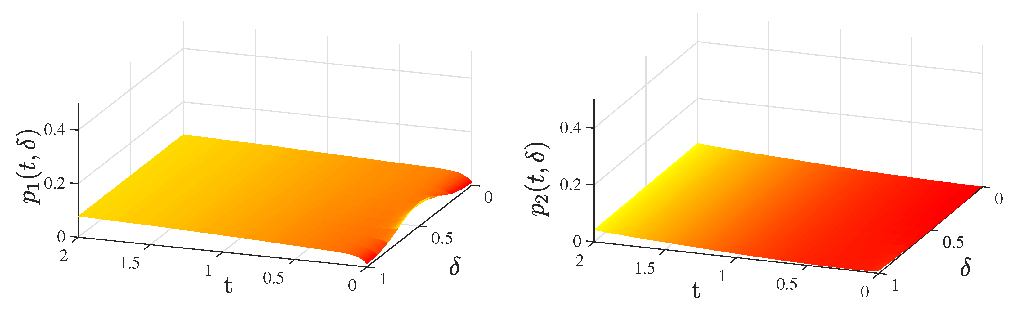
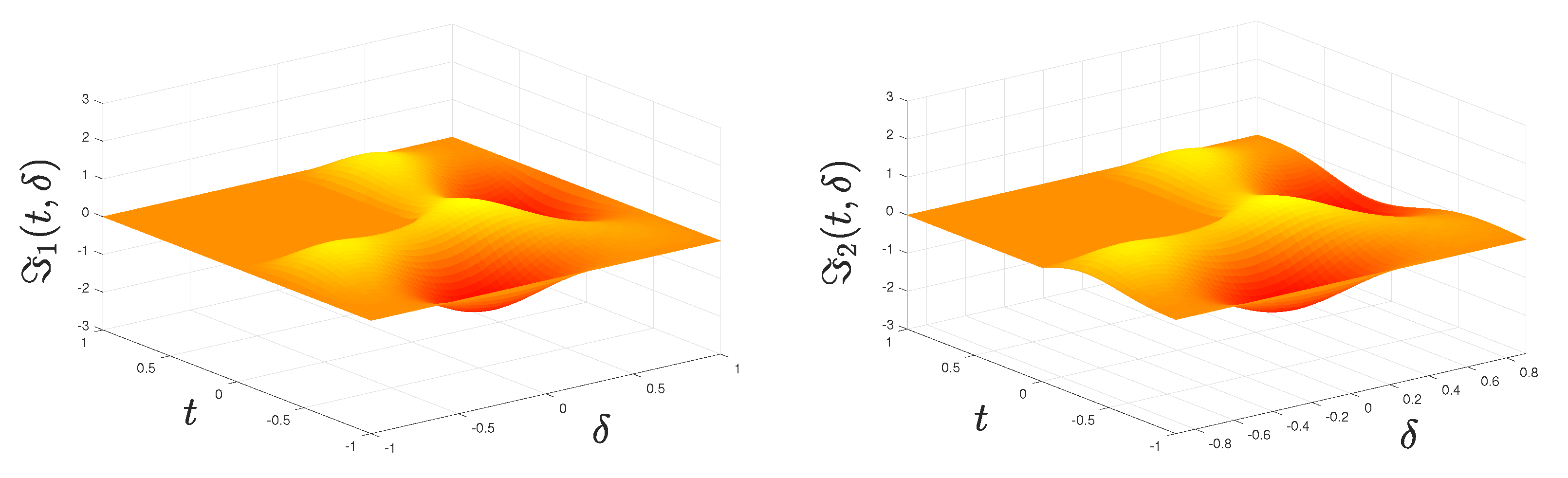
4. Numerical Examples

In order to illustrate the theoretical results, three numerical examples are introduced in this section.
Example 1.
In order to demonstrate the efficiency of Theorem 1, we consider the master fractional-order neural network model with constant and distributed delays and reaction-diffusion terms of type (1)
p φ ( t , δ ) t = l = 1 o δ l ( M φ l p φ ( t , δ ) δ l ) r φ p φ ( t , δ ) + ς = 1 n d φ ς f ς ( p ς ( t , δ ) ) + ς = 1 n s φ ς g ς ( p ς ( t τ , δ ) ) + ς = 1 n a φ ς t L φ ς ( t s ) f ς ( p ς ( s , δ ) ) d s + J φ , φ = 1 , 2 ,
where = 0.98 , n = 2 , o = 1 , Ω = ( 1 , 1 ) , r 1 = 1 , r 2 = 3 , M 11 = M 21 = 1 , τ = 1 , f ς ( p ς ) = g ς ( p ς ) = tanh ( p ς ) , L φ ς = e t , φ , ς = 1 , 2 ,
D = ( d φ ς ) 2 × 2 = d 11 d 12 d 21 d 22 = 0.2 0.1 0.5 0.5 ,
S = ( s φ ς ) 2 × 2 = s 11 s 12 s 21 s 22 = 0.5 0.1 0.2 0.4 ,
A = ( a φ ς ) 2 × 2 = a 11 a 12 a 21 a 22 = 0.4 0.1 0.2 0.3 ,
and the response system of type (3) with pinning controllers of type (7), defined by the feedback, gains k 1 = 1.1 , k 2 = 0 and μ = 1 .
It is easy to verify that Assumption 1 is satisfied for l 1 = l 2 = h 1 = h 2 = 1 , and Assumption 2 is true for γ = 1 . Additionally, the conditions of Lemma 4 are true for A 1 = 1 . Hence, B 1 = B 2 = 1 . In addition, we have that
λ = 4.1 = min 1 φ n 2 ( B φ + r φ + μ k φ ) ς = 1 n l ς | d φ ς | ς = 1 n l φ | d ς φ | ς = 1 n l ς γ | a φ ς | ς = 1 n h ς | s φ ς |
> max 1 φ n h φ ς = 1 n | s ς φ | + l φ ς = 1 n γ | a ς φ | = 1.3 = C .
According to Theorem 1, the master system (19) and response system (3) are globally asymptotically synchronized under the considered pinning controller. The state trajectories of the model (19) without controllers is shown in Figure 1. The trajectories of the corresponding error system are shown in Figure 2, which demonstrates that the master system (19) and response system (3) are globally asymptotically synchronized under the considered pinning controller.
Example 2.
In this example, we consider the master fractional-order neural network model with constant and distributed delays and reaction-diffusion terms of type (1)
p φ ( t , δ ) t = l = 1 o δ l ( M φ l p φ ( t , δ ) δ l ) r φ p φ ( t , δ ) + ς = 1 n d φ ς f ς ( p ς ( t , δ ) ) + ς = 1 n s φ ς g ς ( p ς ( t τ , δ ) ) + ς = 1 n a φ ς t L φ ς ( t s ) f ς ( p ς ( s , δ ) ) d s + J φ , φ = 1 , 2 , 3 ,
where = 0.98 , n = 3 , o = 1 , Ω = ( 1 , 1 ) , r 1 = 1 , r 2 = 3 , r 3 = 4 , M 11 = M 21 = M 31 = 1 , τ = 2 , f ς ( p ς ) = g ς ( p ς ) = tanh ( p ς ) , L φ ς = e t , φ , ς = 1 , 2 , 3 ,
D = ( d φ ς ) 3 × 3 = d 11 d 12 d 13 d 21 d 22 d 23 d 31 d 32 d 33 = 0.2 0.1 0.6 0.5 0.5 0.2 0.4 0.1 0.4 , A = ( a φ ς ) 3 × 3 = a 11 a 12 a 13 a 21 a 22 a 23 a 31 a 32 a 33 = 0.4 0.6 0.2 0.2 0.8 0.1 0.3 0.6 0.2 , S = ( s φ ς ) 3 × 3 = s 11 s 12 s 13 s 21 s 22 s 23 s 31 s 32 s 33 = 0.5 0.6 0.4 0.1 0.7 0.3 0.2 0.8 0.1 ,
and the response system of type (3) with pinning controllers of type (12), defined by the feedback gains k ¯ 1 = 1.5 , k ¯ 2 = 0 , k ¯ 3 = 0.5 , C ( t , δ ) = 0.1 , C ¯ = 1.1 , ϕ = 1 and μ = 1 .
It is easy to verify that Assumption 1 is satisfied for l 1 = l 2 = l 3 = h 1 = h 2 = h 3 = 1 and Assumption 2 is true for γ = 1 . Also, the conditions of Lemma 4 are true for A 1 = 1 . Hence, B 1 = B 2 = B 3 = 1 . In addition, we have
4.3 = min 1 φ n 2 ( B φ + r φ + k ¯ φ μ ( C ( t , δ ) C ¯ ) ϕ ) ς = 1 n l ς | d φ ς | ς = 1 n l φ | d ς φ | ς = 1 n l ς γ | a φ ς | ς = 1 n h ς | s φ ς |
> max 1 φ n h φ ς = 1 n | s ς φ | + l φ ς = 1 n γ | a ς φ | = 4.1 .
Since all conditions of Theorem 2 are satisfied, the master system (20) and response system (3) are globally asymptotically synchronized under the considered pinning controller. The state trajectories of the model (20) without controllers is shown on Figure 3. The trajectories of the corresponding error system are shown on Figure 4, which demonstrates that the master system (20) and response system (3) are globally asymptotically synchronized under the considered pinning controller for τ = 2 .
As it is well known time delay is one the main source of poor performance, oscillation and unstable of the system behaviors. In order to demonstrate the influence of time delay, we consider the cases when τ = 3 and τ = 4 . The oscillation behavior of the error state trajectories for τ = 3 is shown on Figure 5 under the same initial and boundary conditions. Also, for τ = 4 , Figure 6 illustrates the unstable state responses of the error system (8) under the same initial and boundary conditions.
Remark 6.
If in Example 2 the adaptive law (15) is ignored, or ( C ( t , δ ) C ¯ ) ϕ = 0 , then conditions of Theorem 1 cannot be applied since min 1 φ n 2 ( B φ + r φ + μ k φ ) ς = 1 n l ς | d φ ς | ς = 1 n l φ | d ς φ | ς = 1 n l ς γ | a φ ς | ς = 1 n h ς | s φ ς | = 2.3 and max 1 φ n h φ ς = 1 n | s ς φ | + l φ ς = 1 n γ | a ς φ | = 4.1 . Hence, Example 2 again shows that the use of a pinning control together with an adaptive law is essential to reach the control goals.
Example 3.
We consider a higher-dimensional master fractional-order neural network model with constant and distributed delays and reaction-diffusion terms of type (1)
p φ ( t , δ ) t = l = 1 o δ l ( M φ l p φ ( t , δ ) δ l ) r φ p φ ( t , δ ) + ς = 1 n d φ ς f ς ( p ς ( t , δ ) ) + ς = 1 n s φ ς g ς ( p ς ( t τ , δ ) ) + ς = 1 n a φ ς t L φ ς ( t s ) f ς ( p ς ( s , δ ) ) d s + J φ , φ = 1 , 2 , 3 ,
where = 0.99 , n=10, o=2, δ = ( δ 1 , δ 2 ) T Ω R 2 , Ω = { δ 1 , δ 2 ) T : δ l | < 2 , l = 1 , 2 } , r φ = 0.5 , M φ l = 1 , φ , l = 1 , 2 , , 10 , τ = 1 , f ς ( p ς ) = g ς ( p ς ) = 0.5 ( | p ς + 1 | | p ς 1 | ) , L φ ς = e t , φ , ς = 1 , 2 , , 10 ,
D = ( d φ ς ) 10 × 10 = 0.01 0.01 0.02 0.01 0.01 0.01 0.02 0.01 0.01 0.01 0.02 0.01 0.03 0.02 0.02 0.01 0.01 0.02 0.01 0.01 0.01 0.01 0.01 0.01 0.01 0.01 0.01 0.01 0.02 0.01 0.01 0.02 0.01 0.01 0.01 0.01 0.03 0.01 0.01 0.02 0.01 0.01 0.01 0.01 0.01 0.02 0.01 0.01 0.01 0.01 0.02 0.01 0.01 0.01 0.02 0.03 0.01 0.02 0.01 0.03 0.01 0.02 0.03 0.01 0.01 0.01 0.01 0.01 0.01 0.01 0.01 0.01 0.01 0.02 0.01 0.01 0.02 0.01 0.03 0.02 0.02 0.01 0.02 0.03 0.01 0.01 0.01 0.02 0.01 0.03 0.01 0.01 0.01 0.01 0.02 0.01 0.02 0.03 0.01 0.01 , A = ( a φ ς ) 10 × 10 = 0.1 0.1 0.02 0.01 0.2 0.02 0.01 0.01 0.01 0.02 0.1 0.05 0.05 0.2 0.2 0.02 0.2 0.01 0.02 0.03 0.01 0.05 0.04 0.01 0.01 0.01 0.03 0.05 0.03 0.01 0.02 0.05 0.03 0.03 0.01 0.03 0.01 0.03 0.01 0.04 0.05 0.03 0.01 0.04 0.02 0.01 0.05 0.01 0.02 0.05 0.03 0.1 0.03 0.01 0.03 0.08 0.03 0.02 0.03 0.01 0.04 0.02 0.05 0.02 0.01 0.07 0.05 0.01 0.05 0.06 0.01 0.01 0.1 0.03 0.02 0.05 0.02 0.05 0.6 0.01 0.03 0.03 0.07 0.04 0.04 0.06 0.04 0.1 0.01 0.02 0.02 0.02 0.02 0.07 0.01 0.03 0.01 0.04 0.07 0.03 ,
S = ( s φ ς ) 10 × 10 = 0.02 0.1 0.01 0.07 0.03 0.01 0.05 0.02 0.01 0.02 0.01 0.2 0.01 0.01 0.01 0.09 0.06 0.02 0.05 0.03 0.05 0.01 0.2 0.03 0.01 0.08 0.01 0.01 0.06 0.01 0.04 0.03 0.05 0.02 0.02 0.07 0.01 0.02 0.09 0.04 0.03 0.04 0.07 0.02 0.07 0.01 0.02 0.03 0.01 0.03 0.02 0.01 0.09 0.05 0.08 0.01 0.03 0.04 0.03 0.01 0.02 0.03 0.01 0.04 0.01 0.02 0.05 0.01 0.04 0.02 0.05 0.05 0.02 0.03 0.01 0.03 0.01 0.07 0.05 0.01 0.03 0.07 0.02 0.01 0.09 0.04 0.01 0.01 0.06 0.01 0.01 0.03 0.04 0.01 0.08 0.05 0.01 0.02 0.01 0.05 ,
and the response system of type (3) with pinning controllers of type (12), defined by the feedback gains k ¯ φ = 1.5 , φ = 1 , 2 , , 10 , C ( t , δ ) = 0.3 , C ¯ = 1.8 , ϕ = 1 and μ = 1 .
We verify that Assumption 1 is satisfied for l φ = h φ = 1 , φ = 1 , 2 , , 10 , and Assumption 2 is true for γ = 1 . Additionally, the conditions of Lemma 4 hold for A 1 = A 2 = 2 . Hence, B φ = 1 , φ = 1 , 2 , , 10 . In addition, we have
7.36 = min 1 φ n 2 ( B φ + r φ + k ¯ φ μ ( C ( t , δ ) C ¯ ) ϕ ) ς = 1 n l ς | d φ ς | ς = 1 n l φ | d ς φ | ς = 1 n l ς γ | a φ ς | ς = 1 n h ς | s φ ς |
> max 1 φ n h φ ς = 1 n | s ς φ | + l φ ς = 1 n γ | a ς φ | = 1.04 .
Since all conditions of Theorem 2 are satisfied, the master system (21) and response system (3) are globally asymptotically synchronized under the considered pinning controller.

5. Conclusions

In this article, synchronization problems of fractional-order neural systems with time delays, distributed delays and reaction diffusion terms by applying pinning controllers are investigated. Caputo partial fractional derivatives are used in the definition of the model. New and easy verified conditions are derived to reach the synchronization goal of the target model. The conditions are in the form of inequalities between the model’s parameters. In our analysis, special Lyapunov functions with fractional integration terms are constructed, and the Lyapunov method is applied. Numerical examples are also elaborated and demonstrated. It is worth noting that the model derived in this paper is associated with the state variables as well as the effect of the reaction-diffusion terms, which make the results obtained more general. The proposed control method can be further applied to extended impulsive models. Considering the effect of some uncertain terms is also a future direction of research. The established synchronization results can be applied in the study of the robustness behavior of uncertain fractional-order neural network models.

Author Contributions

Conceptualization, M.H., T.F.I., M.S.A., G.S., I.S., B.A.Y. and K.I.O.; methodology, M.H., T.F.I., M.S.A., G.S., I.S., B.A.Y. and K.I.O.; formal analysis, M.H., T.F.I., M.S.A., G.S., I.S., B.A.Y. and K.I.O.; investigation, M.H., T.F.I., M.S.A., G.S., I.S., B.A.Y. and K.I.O.; writing—original draft preparation, I.S. and M.S.A. All authors have read and agreed to the published version of the manuscript.

Funding

This research was partly funded by the Deanship of Scientific Research at King Khalid University under grant number RGP.2/47/43/1443.

Data Availability Statement

Not applicable.

Acknowledgments

The authors extend their appreciation to the Deanship of Scientific Research at King Khalid University for funding this work through large groups (project under grant number RGP.2/47/43/1443.

Conflicts of Interest

The authors declare no conflict of interest.

References

  1. Kilbas, A.; Srivastava, H.M.; Trujillo, J.J. Theory and Applications of Fractional Differential Equations, 1st ed.; Elsevier: New York, NY, USA, 2006; ISBN 9780444518323. [Google Scholar]
  2. Baleanu, D.; Diethelm, K.; Scalas, E.; Trujillo, J.J. Fractional Calculus: Models and Numerical Methods, 1st ed.; World Scientific: Singapore, 2012; ISBN 978-981-4355-20-9. [Google Scholar]
  3. Magin, R. Fractional Calculus in Bioengineering, 1st ed.; Begell House: Redding, CA, USA, 2006; ISBN 978-1567002157. [Google Scholar]
  4. Bukhari, A.H.; Raja, M.A.Z.; Sulaiman, M.; Islam, S.; Shoaib, M.; Kumam, P. Fractional neuro-sequential ARFIMA-LSTM for financial market forecasting. IEEE Access 2020, 8, 71326–71338. [Google Scholar] [CrossRef]
  5. Stamova, I.M.; Stamov, G.T. Functional and Impulsive Differential Equations of Fractional Order: Qualitative Analysis and Applications, 1st ed.; CRC Press/Taylor and Francis Group: Boca Raton, FL, USA, 2017; ISBN 9781498764834. [Google Scholar]
  6. Haykin, S. Neural Networks: A Comprehensive Foundation; Prentice-Hall: Englewood Cliffs, NJ, USA, 1999; ISBN 0132733501/9780132733502. [Google Scholar]
  7. Jahanbakhti, H. A novel fractional-order neural network for model reduction of large-scale systems with fractional-order nonlinear structure. Soft Comput. 2020, 24, 13489–13499. [Google Scholar] [CrossRef]
  8. Zun˜iga Aguilar, C.J.; Gómez-Aguilar, J.F.; Alvarado-Martínez, V.M.; Romero-Ugalde, H.M. Fractional order neural networks for system identification. Chaos Solitions Fractals 2020, 130, 109444. [Google Scholar] [CrossRef]
  9. Kaslik, E.; Sivasundaram, S. Nonlinear dynamics and chaos in fractional order neural networks. Neural Netw. 2012, 32, 245–256. [Google Scholar] [CrossRef] [PubMed]
  10. Lundstrom, B.; Higgs, M.; Spain, W.; Fairhall, A.L. Fractional differentiation by neocortical pyramidal neurons. Nat. Neurosci. 2008, 11, 1335–1342. [Google Scholar] [CrossRef]
  11. Anbalagan, P.; Hincal, E.; Ramachandran, R.; Baleanu, D.; Cao, J.; Niezabitowski, M. A Razumikhin approach to stability and synchronization criteria for fractional order time delayed gene regulatory networks. AIMS Math. 2021, 6, 4526–4555. [Google Scholar] [CrossRef]
  12. Stamov, T.; Stamova, I. Design of impulsive controllers and impulsive control strategy for the Mittag–Leffler stability behavior of fractional gene regulatory networks. Neurocomputing 2021, 424, 54–62. [Google Scholar] [CrossRef]
  13. Kandasamy, U.; Li, X.; Rakkiyappan, R. Quasi-synchronization and bifurcation results on fractional-order quaternion-valued neural networks. IEEE Trans. Neural Netw. Learn. Syst. 2020, 31, 4063–4072. [Google Scholar] [CrossRef]
  14. Song, C.; Cao, J. Dynamics in fractional-order neural networks. Neurocomputing 2014, 142, 494–498. [Google Scholar] [CrossRef]
  15. Cheng, H.; Zhong, S.; Zhong, Q.; Shi, K.; Wang, X. Lag exponential synchronization of delayed memristor-based neural networks via robust analysis. IEEE Access 2019, 7, 173–182. [Google Scholar] [CrossRef]
  16. Lee, S.H.; Park, M.J.; Kwon, O.M.; Selvaraj, P. Improved synchronization criteria for chaotic neural networks with sampled-data control subject to actuator saturation. Int. J. Control Autom. Syst. 2019, 17, 2430–2440. [Google Scholar] [CrossRef]
  17. Zhang, R.; Zeng, D.; Zhong, S.; Shi, K. Memory feedback PID control for exponential synchronization of chaotic Lur’e systems. Int. J. Syst. Sci. 2017, 48, 2473–2484. [Google Scholar] [CrossRef]
  18. Senan, S.; Syed Ali, M.; Vadivel, R.; Arik, S. Decentralized event-triggered synchronization of uncertain Markovian jumping neutral-type neural networks with mixed delays. Neural Netw. 2017, 86, 32–41. [Google Scholar] [CrossRef] [PubMed]
  19. Shi, L.; Zhu, H.; Zhong, S.; Shi, K.; Cheng, J. Cluster synchronization of linearly coupled complex networks via linear and adaptive feedback pinning controls. Nonlinear Dyn. 2017, 88, 859–870. [Google Scholar] [CrossRef]
  20. Syed Ali, M.; Yogambigai, J.; Cao, J. Synchronization of master-slave Markovian switching complex dynamical networks with time-varying delays in nonlinear function via sliding mode control. Acta Math. Sci. Ser. B Engl. Ed. 2017, 37, 368–384. [Google Scholar]
  21. Wang, J.; Shi, K.; Huang, Q.; Zhong, S.; Zhang, D. Stochastic switched sampled-data control for synchronization of delayed chaotic neural networks with packet dropout. Appl. Math. Comput. 2018, 335, 211–230. [Google Scholar] [CrossRef]
  22. Gu, K.; Kharitonov, V.L.; Chen, J. Stability of Time Delay Systems, 2nd ed.; Birkhuser: Boston, MA, USA, 2003; ISBN 978-1-4612-0039-0. [Google Scholar]
  23. Li, X.; Yang, X.; Song, S. Lyapunov conditions for finite-time stability of time-varying time-delay systems. Automatica 2019, 103, 135–140. [Google Scholar] [CrossRef]
  24. Chen, L.; Wu, R.; Chu, Z.; He, Y.; Yin, L. Pinning synchronization of fractional-order delayed complex networks with non-delayed and delayed couplings. Int. J. Control 2017, 90, 1245–1255. [Google Scholar] [CrossRef]
  25. Zhang, W.; Zhang, H.; Cao, J.; Zhang, H.; Chen, D. Synchronization of delayed fractional-order complex-valued neural networks with leakage delay. Phys. A 2020, 556, 124710. [Google Scholar] [CrossRef]
  26. Ali, M.S.; Hymavathi, M. Synchronization of fractional order neutral type fuzzy cellular neural networks with discrete and distributed delays via state feedback control. Neural Process. Lett. 2021, 53, 929–957. [Google Scholar] [CrossRef]
  27. Zhang, Y.J.; Liu, S.; Yang, R.; Tan, Y.Y.; Li, X. Global synchronization of fractional coupled networks with discrete and distributed delays. Phys. A 2019, 514, 830–837. [Google Scholar] [CrossRef]
  28. Lv, X.; Cao, J.; Li, X.; Abdel-Aty, M.; Al-Juboori, U.A. Synchronization analysis for complex dynamical networks with coupling delay via event-triggered delayed impulsive control. IEEE Trans. Cybern. 2021, 51, 5269–5278. [Google Scholar] [CrossRef] [PubMed]
  29. Yang, X.; Li, X.; Lu, J.; Cheng, Z. Synchronization of time-delayed complex networks with switching topology via hybrid actuator fault and impulsive effects control. IEEE Trans. Cybern. 2020, 50, 4043–4052. [Google Scholar] [CrossRef] [PubMed]
  30. Kumar, S.; Matouk, A.E.; Chaudhary, H.; Kant, S. Control and synchronization of fractional-order chaotic satellite systems using feedback and adaptive control techniques. Int. J. Adapt. Control Signal Process. 2021, 35, 484–497. [Google Scholar] [CrossRef]
  31. Padron, J.P.; Perez, J.P.; Pérez Díaz, J.J.; Martinez Huerta, A. Time-delay synchronization and anti-synchronization of variable-order fractional discrete-time Chen–Rossler chaotic systems using variable-order fractional discrete-time PID control. Mathematics 2021, 9, 2149. [Google Scholar] [CrossRef]
  32. Yang, X.; Cao, J.; Yang, Z. Synchronization of coupled reaction- diffusion neural networks with time-varying delays via pinning impulsive controller. SIAM J. Control Optim. 2013, 51, 3486–3510. [Google Scholar] [CrossRef]
  33. Lagergren, J.H.; Nardini, J.T.; Baker, R.E.; Simpson, M.J.; Flores, K.B. Biologically informed neural networks guide mechanistic modeling from sparse experimental data. PLoS Comput. Biol. 2020, 16, e1008462. [Google Scholar] [CrossRef]
  34. Stamov, G.; Stamova, I.; Spirova, C. Impulsive reaction-diffusion delayed models in biology: Integral manifolds approach. Entropy 2021, 23, 1631. [Google Scholar] [CrossRef] [PubMed]
  35. Lv, Y.; Hu, C.; Yu, J.; Jiang, H.; Huang, T. Edge-based fractional-order adaptive strategies for synchronization of fractional-order coupled networks with reaction-diffusion terms. IEEE Trans. Cybern. 2020, 50, 1582–1594. [Google Scholar] [CrossRef]
  36. Stamova, I.; Stamov, G. Mittag–Leffler synchronization of fractional neural networks with time-varying delays and reaction-diffusion terms using impulsive and linear controllers. Neural Netw. 2017, 96, 22–32. [Google Scholar] [CrossRef]
  37. Yin, W.; Liu, S.; Wu, X. Synchronization of fractional reaction-diffusion neural networks with time-varying delays and input saturation. IEEE Access 2021, 9, 50907–50916. [Google Scholar]
  38. Li, B.; Wang, N.; Ruan, X.; Pan, Q. Pinning and adaptive synchronization of fractional-order complex dynamical networks with and without time-varying delay. Adv. Differ. Equ. 2018, 2018, 6. [Google Scholar] [CrossRef] [Green Version]
  39. Tang, Y.; Wang, Z.; Fang, J. Pinning control of fractional-order weighted complex networks. Chaos 2009, 19, 013112. [Google Scholar] [CrossRef]
  40. Wang, J.; Ma, Q.; Chen, A.; Liang, Z. Pinning synchronization of fractional-order complex networks with Lipschitz-type nonlinear dynamics. ISA Trans. 2015, 57, 111–116. [Google Scholar] [CrossRef] [PubMed]
  41. Xai, H.; Ren, G.; Yu, Y.; Xu, C. Adaptive pinning synchronization of fractional complex networks with impulses and reaction-diffusion terms. Mathematics 2019, 4, 405. [Google Scholar]
  42. Delavari, H.; Baleanu, D.; Sadati, J. Stability analysis of Caputo fractional-order nonlinear systems revisited. Nonlinear Dyn. 2012, 67, 2433–2439. [Google Scholar] [CrossRef]
  43. Duatte-Mermound, M.A.; Aguila-Camacho, N.; Gallegos, J.A.; Castro-Limares, R. Using general quadratic Lyapunov functions to prove Lyapunov uniform stability of fractional order systems. Commun. Nonlinear Sci. Numer. Simul. 2015, 22, 650–659. [Google Scholar] [CrossRef]
  44. Liang, S.; Wu, R.; Chen, L. Comparision principles and stability of nonlinear fractional-order cellular neural networks with multiple time delays. Neurocomputing 2015, 168, 618–625. [Google Scholar] [CrossRef]
  45. Lu, J.G. Global exponential stability and periodicity of reaction-diffusion delayed recurrent neural networks with Dirichlet boundary conditions. Chaos Solitions Fractals 2008, 35, 116–125. [Google Scholar] [CrossRef]
Figure 1. The state trajectories of System (19) without controllers.
Mathematics 10 03916 g001
Figure 2. The state trajectories of the error system (8) in Example 1 with controller (7).
Mathematics 10 03916 g002
Figure 3. The state trajectories of the system (20) without controller.
Mathematics 10 03916 g003
Figure 4. The state trajectories of the corresponding error system of the type (8) in Example 2 with controller (7) for τ = 2 .
Mathematics 10 03916 g004
Figure 5. The state trajectories of the corresponding error system of the type (8) in Example 2 with controller (7) for τ = 3 .
Mathematics 10 03916 g005
Figure 6. The state trajectories of the corresponding error system of the type (8) in Example 2 with controller (7) for τ = 4 .
Mathematics 10 03916 g006
Publisher’s Note: MDPI stays neutral with regard to jurisdictional claims in published maps and institutional affiliations.

