OCPHN: Outfit Compatibility Prediction with Hypergraph Networks

Abstract

With the rapid development of the online shopping, the pursuit of outfit compatibility has become a basic requirement for an increasing number of customers. The existing work on outfit compatibility prediction largely focuses on modeling pairwise item compatibility without considering modeling the whole outfit directly. To address the problem, in this paper, we propose a novel hypergraph-based compatibility modeling scheme named OCPHN, which is able to better model complex relationships among outfits. In OCPHN, we represent the outfit as a hypergraph, where each hypernode represents a category and each hyperedge represents the interactions between multiple categories (i.e., they appear in the same outfit). To better predict outfit compatibility, the hypergraph is transformed into a simple graph, and the message propagation mechanism in the graph convolution network is used to aggregate the neighbours’ information on the node and update the node representations. Furthermore, with learned node representations, an attention mechanism is introduced to compute the outfit compatibility score. Using a benchmark dataset, the experimental results show that the proposed method is an improvement over the strangest baselines in terms of accuracy by about 3% and 1% in the fill-in-the-blank and compatibility prediction tasks, respectively.

1. Introduction

In recent years, online shopping has become more and more important for modern consumers and has greatly promoted the development of the fashion industry. According to Statista, the global online fashion market was worth 533 billion dollars in 2018, and it is predicted to grow to 825 billion dollars by 2022. In 2018, apparel accounted for 65 percent of the market, followed by footwear (25 percent) and bags and accessories (10 percent). Additionally, there are several interactive fashion community sites that allow customers to create their own styles using the image data on the site. The typical industrial sites are Polyvore (https://www.polyvore.com) (accessed on 20 August 2022), Farfetch (https://www.farfetch.cn) (accessed on 20 August 2022) and Dappei (https:/dappei.cn) (accessed on 20 August 2022). However, not everyone is a natural fashion designer. Therefore, it is of great significance to establish a reasonable and effective outfit compatibility prediction model by analyzing the masses of fashion items and outfits.

Outfit compatibility is a complex task, and it is fundamental to a variety of industry applications such as personalized fashion design [1,2,3], fashion analysis [4], item recommendation [5,6] and fashion trend forecasting [7,8]. The key to outfit compatibility is to measure the degree of matching of fashion items in an outfit. Figure 1 shows examples of compatible and incompatible fashion outfits.

In fact, a great amount of recent work on fashion matching has been devoted to addressing the task of predicting fashion compatibility. Previous works [9,10] all relied on mapping the items to a style space and calculating the distance of the items’ style vectors to represent the compatibility. The disadvantage of these approaches is that each pair of items considered is handled independently, which means the final prediction relies on isolated comparisons between the characteristics of each item. However, the outfit compatibility is determined by the characteristics of the pairs of items and affected by the characteristics of other items in the same outfit.

Therefore, the key to solving outfit compatibility modeling is how to represent the overall outfits properly, rather than just focusing on pairs of items. In recent years, some studies have used graph deep learning to tackle some complicated relations and interoperability problems in outfit compatibility. Although these approaches using GNNs have achieved successful results in compatibility modeling, they essentially establish the relationship or connection between two nodes. However, such pairwise connection is not always appropriate in practical application. In actual situations, the relationships between multiple nodes are often more complicated than the pairwise connection between two nodes. For example, outfit compatibility is determined by multiple items and not just pairs of items.

To solve the limitations, one possible method is to use a hypergraph to describe such complex relationships. Based on the above statements, in this paper, we focus on outfit compatibility prediction for fashion matching and propose a novel model (OCPHN) to better model the relationships between items and outfits. It can better predict the compatibility of the outfits from the hypergraph.

Our proposed scheme is shown in Figure 2. In OCPHN, we propose a new form of outfit representation: hypergraph representation. In particular, we construct a fashion hypergraph based on the Polyvore dataset, where each hypernode represents a category and each hyperedge represents the interactions between multiple categories (i.e., they appear in the same outfit). Then, a convolutional neural network is used to extract the visual features of each item and learn the category features corresponding to each node through the model. For each hyperedge in the fashion hypergraph, we maximize the total differences among multiple nodes by combining the visual features and category features of each hypernode, and then the two nodes with the greatest differences are selected to represent the hyperedge. The remaining nodes in the hyperedge act as a medium connection with the two selected nodes to form a simple graph. Benefitting from the message propagation rules in the GNN, the nodes’ representation can be iteratively updated by aggregating the neighbor nodes’ embeddings. With the learned node representations, an attention mechanism is utilized to calculate the output of the two selected nodes as the outfit compatibility score.

We validated our model in the following two tasks: (1) fill-in-the-blank, where an item is selected from multiple choices that is compatible with other components in outfits that have one missing item, and (2) compatibility prediction, where the compatibility scores of given fashion outfits are predicted. Extensive experiments are conducted on a real-world dataset to demonstrate the effectiveness of our proposed method compared with state-of-the-art methods. The code of our work has been released. (https://github.com/outfit-net/outfit-commpatibility) (accessed on 20 August 2022).

Our main contributions in this work can be summarized as follows:

• To the best of our knowledge, this is the first attempt to introduce the hypergraph for outfit compatibility prediction. Compared with the existing models using sequence representation or graph representation for compatibility prediction, our model can perform more intuitive and sophisticated modeling of complex relationships.
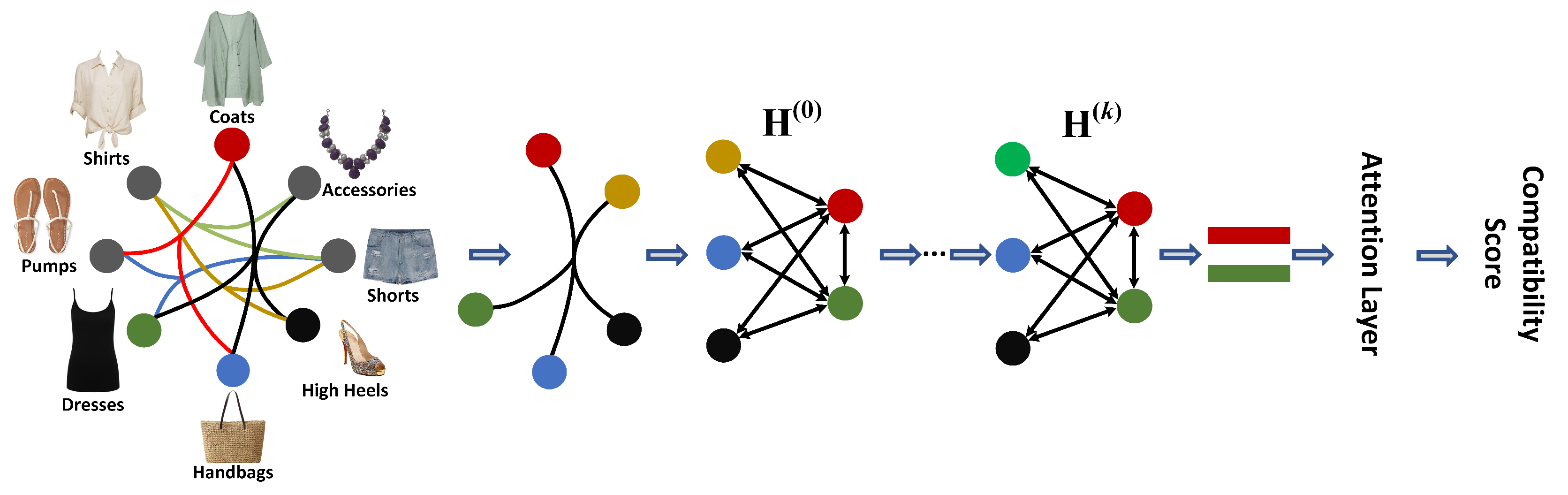
• We propose a novel method, OCPHN, which can model multiple nodes’ interactions in the hypergraph and learn node representations better. With OCPHN, we can not only model outfit compatibility from visual features and category features but also use the attention mechanism to enhance the representation ability of our model.
• By conducting extensive experiments on a real-world dataset (Polyvore dataset), we demonstrate that our proposed model outperforms the baselines.

2. Related Work

In this section, we introduce the related tasks in our work, namely fashion compatibility modeling, and explain the proposed approach in relation to existing works briefly.

Fashion Compatibility Modeling

Currently, fashion compatibility prediction [11,12,13,14] has attracted increasing attention because it is the key to fashion recommendation. To measure their compatibilities, McAuley et al. [15] learned a distance metric between clothes with CNN features. Veit et al. [16] further proposed to learn the distance metric with an end-to-end trained Siamese network. In addition, Han et al. [17] used multiple layer perception (MLP) to find a latent space and model the complex interactions between items accurately. Some other works [18,19] focused on the importance of exploiting multi-modality features in fashion-related tasks. For instance, Li et al. [20] trained an RNN to predict the popularity of a fashion set by fusing text and image features. Song et al. [21] proposed a Bayesian personalized ranking dual autoencoder (BPR-DAE) model to learn a latent compatibility space by utilizing multiple modalities (e.g., visual and contextual modalities). However, these works only focused on mapping the pairwise items to the style space and estimating the compatibility of pairwise items instead of the whole outfit.

In recent years, some work has been devoted to modeling the compatibility of the whole outfit. For example, Han et al. [22] considered a fashion outfit to be an ordered sequence of products and exploited bidirectional LSTMs to predict the next item sequentially with and conditionally on previous ones to learn their compatibility relationships. This method was improved by adding a new type of style embedding for the full outfit [23]. Vasileva et al. [9] also used textual information to improve the product embeddings, along with using conditional similarity networks [24] to produce type-conditioned embeddings and learn a metric for compatibility. Following that, Cui et al. [25] utilized category information to represent the outfit as a graph to model complex relations among items and introduced an attention mechanism. Cucurull et al. [26] proposed the graph autoencoder to regard the outfit compatibility problem as an edge prediction problem and improved the performance of using a graph neural network to predict outfit compatibility by incorporating context information. However, all the aforementioned studies only considered the relationship between the pair’s items and ignored the relationships between multiple items.

Therefore, in this work, the hypergraph is introduced to represent the outfit. A hypergraph is a generalized concept that can express complex relational networks. It is different from the traditional graph where edges can only connect two nodes, as the hyperedges in a hypergraph can connect any number of nodes. In this way, more complicated and higher-level relationships among nodes can be represented by a hypergraph. We prove that this method is more effective than sequence representation and graph representation.

3. Technical Background

In this section, we review the technical background on graph neural networks and hypergraph learning.

3.1. Graph Neural Network

A graph neural network (GNN) is a type of structure to model a set of elements (nodes) and their relationships (edges). Recently, research analyzing graphs with machine learning [27,28,29] has been receiving more and more attention because of the great representation power of graphs.

The notion of a graph neural network was initially outlined by Gori et al. [30] and further elaborated upon by Scarselli et al. [31] and Gallicchio et al. [32]. A GNN can be applied on most kinds of graphs, including directed, undirected and cyclic graphs. A GNN learns a target node’s representation by propagating the neighbouring information in an iterative manner until a stable fixed point is reached. There have been many variants of GNNs with various kinds of aggregators and updaters proposed these days. For instance, Li et al. [33] proposed a gated graph neural network (GGNN) by introducing gated recurrent units (GRUs) in the propagation process for updating. The graph convolution network (GCN) [34] was proposed by Kipf et al. and can perform a convolution on the graph and aggregate the information derived from all the neighbours to update the node embeddings. Distinct from GCNs, Hamilton et al. proposed GraphSAGE [35], which updates the node embedding by uniformly sampling and aggregating features from its local neighbours. Velickovic et al. proposed the graph attention network (GAT) [36] to incorporate the attention mechanism into the propagation step to better aggregate the neighbouring information. Recently, due to convincing performance and high interpretability, the GNN has been widely used in fashion analysis and fashion recommendation.

3.2. Hypergraph Learning

Because hyperedges can connect different numbers of nodes rather than connect only two nodes, hypergraphs have been used as generalized representations of conventional graphs. Due to this flexibility of hypergraphs, the hypergraph structure has been employed to model high-order correlation among data in many computer vision tasks.

Hypergraph learning was first introduced by Zhou et al. [37] as a label propagation method for semi-supervised learning. This method aims to minimize the label differences among vertices with a stronger connection on a hypergraph. It was shown that hypergraph-based learning outperformed graph-based learning in several clustering, embedding and classification tasks. In addition to learning label propagation on hypergraphs, Feng et al. proposed the hypergraph neural network (HGNN) [38], which introduced hypergraph-based representation learning into deep learning. The design of HyperGCN [39] was motivated by the graph convolutional network, which suggested a more efficient and faster model for the same tasks as in the HGNN. Following that, Jiang et al. proposed the dynamic hypergraph neural network [40], which uses the K-NN and k-means clustering methods to construct a hypergraph structure of data without defining the hypergraph structure explicitly. Deep hypernetwork embedding (DHNE) [41] and HyperSAGNN [42] encode networks with hypergraphs to represent data with complicated structures.

4. Proposed Method

In this section, we first formulate the problem and then present our method in detail, which is equipped with three components: (1) model preparation, which extracts the visual features of the image of items and constructs the fashion hypergraph, (2) hypergraph convolution, which initializes the node embeddings and refines the node embeddings via a neural network; that is, it converts the hypergraph into a simple graph and utilizes a GCN to update the outfit representation by aggregating neighbours’ information, and (3) model prediction, which outputs the prediction score for outfit compatibility prediction.

4.1. Problem Formulation

To find an appropriate outfit, people are more likely to opt for high-compatibility clothes, such as a denim bomber jacket, white short sleeves and skinny jeans. Therefore, outfit compatibility can be considered as a summary after comparing each item with others in different aspects (e.g., color, texture and style). The key to outfit compatibility prediction is to model the sophisticated interactions between items and outfits. In this paper, we focus on tacking the essential problem of compatibility modeling for clothing matching. We had a set of outfits $\mathcal{S}=\left\{s_1,s_2,\dots ,s_m\right\}$ in the training set. Given an outfit s consisting of |s| items in the training set, we aim to calculate the outfit compatibility score and predict whether the outfit is compatible.

4.2. Model Preparation

4.2.1. Feature Extraction

As shown in Figure 1, the fashion item image contains the most important information required for outfit composition, and the item image feature is extracted with an advanced deep convolution neural network (ConvNets). This method has been proven effective in image representation learning [43,44]. There are many ConvNets architectures to choose from, and we used the GoogleNet InceptionV3 model for simplicity. In this work, the images of items are fed into the model, and the visual features are output by a linear layer. The dimension count of the visual features of each item was 2048. We utilized the extracted visual features to model the holistic compatibility of the outfit.

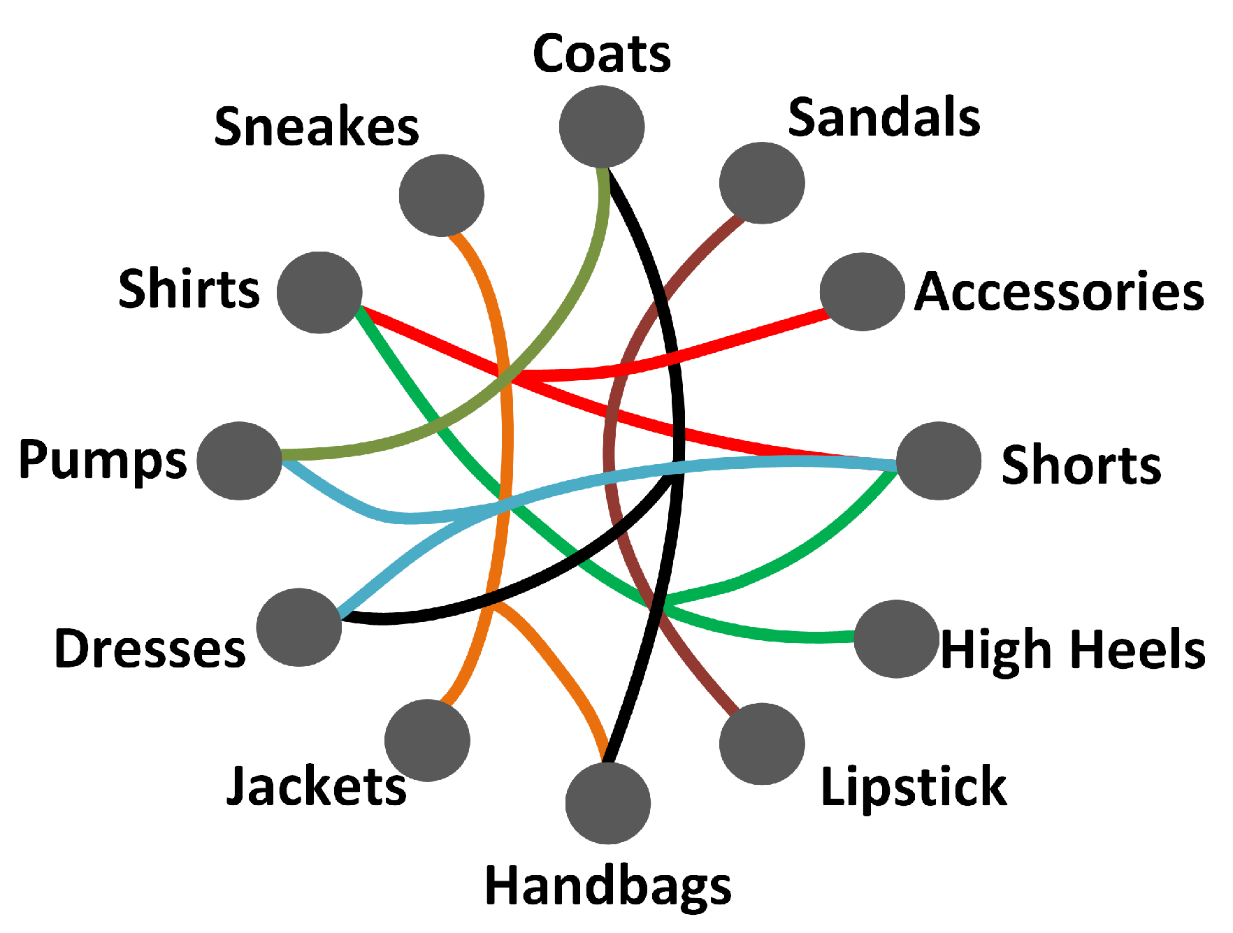
4.2.2. Hypergraph Construction

Based on the training dataset, we constructed a fashion hypergraph $\mathcal{H}=(\mathcal{V},\mathcal{E})$, where the category information of items serves as the prior knowledge of items, as shown in Figure 3. In particular, each circle is assigned only one specific category, and the hyperedge (i.e., the links of the same color) represents the matching interaction between multiple categories (i.e., they appear in the same outfit). Therefore, if each item is filled into its corresponding nodes, then each outfit can be described as a hyperedge of a hypergraph.

After constructing the fashion hypergraph, we first converted each hyperedge into a simple graph by maximizing the differences between multiple nodes. Then, we used OCPHN to better predict the outfit compatibility from the hypergraph as described in the next section.

4.3. Hypergraph Convolution

4.3.1. Node Initialization

The input of our model is the visual features ${\mathbf{r}}_i$ of items extracted through the neural network. Meanwhile, taking into account the differences between different categories, a learning variable ${\mathbf{c}}_i$ (i.e., the category features) is set for each category. The visual features and category features can be used to initialize the state of their corresponding nodes. In this paper, each item was filled into its corresponding node. Then, the multiple layer perceptron (MLP) is adopted to map the visual features and category features of each node to a common style space, and the size of the style space is d. To better represent each node, the two representations in the style space concatenate as the state representation of each node. Therefore, the initialization representation of each node in the style space is as follows:

$${\mathbf{f}}_i=MLP\left({\mathbf{r}}_i\right)\parallel MLP\left({\mathbf{c}}_i\right),$$

(1)

where MLP is a three-layer architecture consisting of a LeakyReLU [45] nonlinear layer and two tanh nonlinear layers. Aside from that, the size of the node state is two d.

4.3.2. Converting a Hyperedge to a Graph

Different items have different weighted interactions with others in the outfit. To capture the interactions between different items in an outfit, a given outfit containing |m| items and their features in the style space can be denoted as a set $\mathcal{F}=\left\{{\mathbf{f}}_1,{\mathbf{f}}_2,\dots ,{\mathbf{f}}_m\right\}$, where ${\mathbf{f}}_i$ is the feature vector for the ith item in the outfit. The similarities among items can be represented in matrix form:

$$\mathbf{R}=\left[\begin{array}{cccc}{r}_{11}& r_{12}& \cdots & r_{1m}\\ r_{21}& r_{22}& \cdots & r_{2m}\\ ⋮& ⋮& \ddots & ⋮\\ r_{m1}& r_{m2}& \cdots & r_{mm}\end{array}\right],$$

(2)

here, $r_{ij}$ is the similarity between the features of the ith item and the features of the jth item, which is an undirected relationship expressed formally as $r_{ij}=r_{ji}$. At the same time, the diagonal elements in the R matrix represent the items’ self-similarity in the outfit. To obtain only the similarity between different items, the R matrix is slightly transformed to remove the redundant content. The new matrix is represented by

$${\mathbf{R}}_d=\left[\begin{array}{cccc}{r}_{12}& r_{13}& \cdots & r_{1m}\\ 0& r_{23}& \cdots & r_{2m}\\ ⋮& ⋮& ⋮& ⋮\\ 0& 0& \cdots & r_{(m-1)m}\end{array}\right]$$

(3)

In our model, the outfit is denoted as a hyperedge ${\mathcal{E}}_i=\left\{e_1,e_2,\dots ,e_m\right\}$, where $e_t$ is the tth node in the hyperedge. Therefore, the non-zero elements in the ${\mathbf{R}}_d$ matrix can be regarded as the similarity between different nodes in the hyperedge. We selected the two nodes with the largest signal characteristics from the hyperedge containing multiple nodes and represented the whole hyperedge through the link between the two nodes. Therefore, the two most different nodes obtained by selecting the smallest element in the ${\mathbf{R}}_d$ matrix are called key nodes, which are expressed as follows:

$$\mathit{let}\left(e_i,e_j\right):=arg\underset{{\mathrm{e}}_i,{\mathrm{e}}_j\in \mathcal{V}}{min}\left|{\mathbf{R}}_d\right|,$$

(4)

where $\left(e_i,e_j\right)$ denotes the simple edge connected by the two most different nodes in the hyperedge.

In the process of transforming the hyperedge, only two nodes are selected for each hyperedge to represent the entire hyperedge, which causes a loss of information for other nodes in the hyperedge. To make full use of all the nodes’ information, the remaining nodes, which are called mediator nodes, are connected with the key nodes to form a new simple graph. As shown in Figure 4, each mediator node connects two key nodes.

4.3.3. State Propagation Updates the Node Status

Based on the GGNN, OCPHN is designed to model node interactions on a simple graph by transforming a hypergraph. It can model the interactions flexibly and explicitly. In OCPHN, each node has a hidden state vector. Then, the graph convolution network (GCN) is utilized to learn node representation by smoothing the features on the graph. The nodes aggregate the state information of neighbours into a new representation by performing graph convolution iteratively. The representation of nodes is expressed as follows:

$${\mathbf{f}}_u^{\left(k\right)}=\sum _{{\mathrm{e}}_i,{\mathrm{e}}_u\in \mathcal{V}}\mathbf{A}\left(\mathbf{W}{\mathbf{f}}_i^{(k-1)}+\mathbf{b}\right),$$

(5)

where ${\mathbf{f}}_u^{\left(k\right)}$ denotes the state of node ${\mathrm{e}}_u$ in the kth propagation step, $\mathbf{W}\in {\mathbb{R}}^{2d\times 2d}$ and $\mathbf{b}\in {\mathbb{R}}^{2d\times 1}$ are the trainable weight matrix and biases matrix, respectively, for distilling useful information for propagation, and A is the adjacency matrix, which can reflect the connected relation of nodes, where A is equal to one if node $e_i$ has interaction with node $e_u$; otherwise, it is zero. Apparently, the weight matrix W and the adjacency matrix A decide the node interactions. The traditional GGNN is unable to model flexible and complex interactions. Therefore, it is essential to provide a unique weight matrix for each interaction. However, if a unique weight matrix and a biases matrix are assigned to each interaction simply, then they will consume too much parameter space and running time. To remedy the problem, each node is assigned to an input weight matrix and an input biases matrix, as well as an output weight matrix and an output biases matrix. When node $e_i$ sends its state information to node $e_u$, the state information will first be transformed by its output matrix and then be transformed by node $e_u$ ’s input matrix before $e_u$ receives it. The new representation of the nodes is expressed as follows:

$${\mathbf{f}}_u^{\left(k\right)}=\sum _{{\mathrm{e}}_i,{\mathrm{e}}_u\in \mathcal{V}}\mathbf{A}\left({\mathbf{W}}_2\left({\mathbf{W}}_1{\mathbf{f}}_i^{(k-1)}+{\mathbf{b}}_1\right)+{\mathbf{b}}_2\right),$$

(6)

where ${\mathbf{W}}_1\in {\mathbb{R}}^{2d\times 2d}$ and ${\mathbf{b}}_1\in {\mathbb{R}}^{2d\times 1}$ denote the output weight matrix and the output biases matrix, respectively, and ${\mathbf{W}}_2\in {\mathbb{R}}^{2d\times 2d}$ and ${\mathbf{b}}_2\in {\mathbb{R}}^{2d\times 1}$ denote the input weight matrix and the input biases matrix, respectively.

After summarizing the state information of the neighbours, each node updates its final representation via GRUs as follows:

$${\mathbf{h}}_u^{\left(k\right)}=\mathit{GRU}\left({\mathbf{h}}_u^{(k-1)},{\mathbf{f}}_u^{\left(k\right)}\right),$$

(7)

where ${\mathbf{h}}_u^{\left(k\right)}$ is the final representation of node $e_u$ after k instances of propagation.

4.4. Model Prediction

To estimate whether multiple fashion items form good outfits, the outfits’ compatibility scores were calculated by utilizing the final representations of the items. Since each item representation was obtained by aggregating the state information of different neighbours, they had different importance to the outfit. For example, as shown in Figure 1, the white sweater determined the holistic style of the outfit, so its influence on the outfit was more important than the bag. As such, we aimed to model the influence of different items on the outfit compatibility via a self-attention mechanism as follows:

$${\mathrm{m}}_u=\sigma \left({\mathbf{W}}_3{\mathbf{h}}_u^{\left(k\right)}\right),$$

(8)

$${\mathrm{n}}_u=\mu \left({\mathbf{W}}_4{\mathbf{h}}_u^{\left(k\right)}\right),$$

(9)

where ${\mathbf{W}}_3\in {\mathbb{R}}^{1\times 2d}$ and ${\mathbf{W}}_4\in {\mathbb{R}}^{1\times 2d}$ are two trainable weight matrices, $\sigma (·)$ and $\mu (·)$ are set as LeakyReLU and sigmoid activation functions, respectively, ${\mathrm{n}}_u$ refers to the attention weight of item u in the outfit (i.e., the importance of the item to outfit compatibility) and ${\mathrm{m}}_u$ is the compatibility score of item u in the outfit. In OCPHN, we utilize the two most different items in the outfit to represent the whole outfit. Therefore, the outfit compatibility score is represented by calculating the sum of the scores of the two most different items. Finally, we used the inner product to estimate the outfit compatibility score as follows:

$${\widehat{C}}_s={\mathrm{m}}_u{\mathrm{n}}_u^{\top }+{\mathrm{m}}_o{\mathrm{n}}_o^{\top },$$

(10)

where ${\widehat{C}}_s$ is the outfit compatibility score by adding the compatibility scores of the two most different items u and item o. In our work, we mainly discuss the weight matrix learning, so only a simple interaction function of the inner product was employed. Other more complicated choices, such as the neural network-based interaction function, were left for our future work.

4.5. Optimization

In this part, we introduce the objective function for our model and model size.

4.5.1. Objective Function

To better learn the outfit compatibility, we adopted the Bayesian personalized ranking (BPR) algorithm [46] for both tasks, which has been used intensively in recommender systems. Specifically, BPR assumes that the observed outfits are assigned to higher prediction values than unobserved ones. The objective function is as follows:

$${\mathcal{L}}_{bpr}=\sum _{\left(s,s^{-}\right)\in \mathcal{Z}}-ln\eta \left({\widehat{C}}_s-{\widehat{C}}_{s^{-}}\right)+\lambda {\parallel \mathsf{\Theta }\parallel }_2^2,$$

(11)

where $\mathcal{Z}=\left\{\left(s,s^{-}\right)\right\}$ is the training data for compatibility learning, each pair $\left(s,s^{-}\right)$ indicates an observed outfit s (i.e., positive samples) and an unobserved outfit $s^{-}$ (i.e., randomly generated negative samples), $\Theta$ denotes all the trainable model parameters, $\lambda$ controls the $L_2$ regularization strength to prevent overfitting and $\eta (·)$ is the sigmoid function.

4.5.2. Parameter Space

The parameters that need to be learned mainly consist of the parameters correlated to nodes and the perception network in the attention mechanism. For each node, we first set a category vector to obtain the key node of the hyperedge by utilizing an MLP network. Then, we had an input matrix and an output matrix to propagate the state information for each node. In total, we had $\left(2m+3d{d}^{\prime }\right)$ matrices, which was proportional to the number of nodes m. Aside from that, we had two matrices of a perception network in the attention mechanism. Overall, there were $O\left(2m+5d{d}^{\prime }\right)$ matrices.

5. Experiment

To evaluate the effectiveness of OCPHN, in this section, we conduct extensive experiments. We first introduce the data that are collected and used for our experiment. Then, we show the experiment settings and the performance of the proposed model in two tasks: fill-in-the-blank and outfit compatibility prediction, which are then compared with the state-of-the-art models.

5.1. Dataset

The existing Polyvore dataset was collected from a popular fashion website Polyvore.com, which allows their members to create fashion outfits from different items or like and save outfits created by others. It contains 164,379 items that make up 21,899 different outfits. These outfits were split into 17,316 for training, 1497 for validation and 3076 for testing. Meanwhile, we used a graph segmentation algorithm to ensure there were no overlapping items between the three splits. Each item contained rich information, such as image information, text descriptions, and categories (e.g., sweaters or skirts). We only used the image information of the items in this paper.

The Polyvore-N [25] dataset was generated from the original Polyvore dataset. In this dataset, the categories that appear less frequently (such as lipstick and furniture) in the original dataset were removed, and only the categories which appeared more than 100 times remained, totaling 120. Meanwhile, to ensure the integrity of the outfits, the outfits consisting of less than three items were filtered out.

Based on the Polyvore-N dataset, we generated a new dataset: Polyvore-N1. We found that some categories were repeated in the Polyvore-N dataset, such as boots appearing twice, so we built a new dataset to ensure the unity of the dataset by removing the categories that were repeated. Meanwhile, we also found that if the number of items in an outfit exceeds eight, then this meant that the outfit contained many duplicate items. To ensure the non-repeatability of the items, we removed outfits with more than eight items. The statistics of the filtered dataset are shown in

Table 1. Statistics of the datasets.

Dateset	Training	Validation	Testing	Items	Outfits	Categories
Polyvore-N	16,983	1294	2697	130,901	20,871	120
Polyvore-N1	16,233	1239	2594	122,708	20,066	100

.

For each dataset, we randomly split them using the ratio $8:1:1$ and divided them into a training set, validation set and testing set. For the training set, we adopted a negative sampling strategy to create the triplets for parameter optimization. The validation set and testing set were applied to tune the hyperparameters and evaluate the performance in the experiments, respectively.

5.2. Experiment Settings

We implemented our OCPHN model in Tensorflow. We performed a grid search strategy to tune the hyperparameters for our model and baselines [47,48]. We searched for the batch size and style space dimension in $\{8,12,16,20,24\}$, searched for the propagation step in $\{0,1,2,3\}$ and tuned the $L_2$ regularization in $\{0.01,0.001,0.0001\}$ and learning rate in $\{0.001,0.0005,0.0001,0.00005\}$. Moreover, we adopted the Adam optimizer to optimize the prediction model and update the model parameters. Additionally, the optimization of the model parameters used the gradients of the loss function. All the experiments were trained on a server equipped with a Quadro M4000 graphics processor. The training stopped until the objective functions converged or until the maximum number of epochs was reached.

5.3. Tasks

The performance of our model was evaluated in two tasks: fill-in-the-blank accuracy and outfit compatibility prediction, expressed by the AUC.

5.3.1. Fill in the Blank (FITB)

The fill-in-the-blank task is a standard test conducted extensively in fashion compatibility research. The task aims to select an item from multiple choices that is compatible with other items to fill in the vacancies in an outfit, as Figure 5 shows. For each outfit in the test dataset, we selected one item randomly and masked it with a blank before selecting three items from other outfits randomly along with the masked item to form a multiple-choice set. We set the masked item as the ground truth, and the masked item was more compatible than the randomly selected one. The performance of this task is evaluated by the accuracy of selecting the right items from the four candidates (FITB accuracy), which is 25% by random selection.

5.3.2. Compatibility Prediction

The compatibility prediction task is used to predict whether an outfit is compatible or not. To evaluate the performance, we first built the compatible outfit set based on the dataset. Then, we produced the same number of incompatible outfits as the compatible outfits for a balanced test set by selecting fashion items randomly from the compatible outfit set. In this task, an outfit was scored for whether its constituting items were compatible with each other. Moreover, we adopted the area under the ROC curve (AUC) metric, which is widely used to evaluate performance.

5.4. Baseline

To demonstrate the effectiveness, we compared our proposed OCPHN with the following methods:

• Random: A model based on random guesses.
• Bi-LSTM [22]: Bi-LSTM regards an outfit as an ordered sequence, and it applies a bidirectional LSTM to predict the next item and learn the outfit compatibility. The method only focuses on visual information. The experimental results are influenced by the memory limitation of the graphics card.
• VCP [26]: VCP is a method that predicts compatibility between two items based on their visual features and context. They define context as the products that are known to be compatible with each of these items. The method only focuses on visual information.
• GGNN [33]: A GGNN uses a graph neural network to model the relationships between outfits and items and calculate the outfit compatibility.
• NGNN [25]: An NGNN utilizes the category information to represent the outfit as a graph and updates the node status information through the graph conventional network and the GRU unit. An NGNN uses the attention mechanism to calculate the graph-level output as an outfit compatibility score. We only focused on the visual features of this method in our experiment.

5.5. Model Comparison

5.5.1. Performance Comparison

We evaluated the performance of OCPHN by conducting comparison experiments with the fill-in-the-blank and compatibility prediction tasks. The results are shown in

Table 2. The performance of models evaluated by fill-in-the-blank accuracy and compatibility prediction expressed as the AUC.

Method	Accuracy (FITB)		AUC (Compatibility Prediction)
	Polyvore-N	Polyvore-N1	Polyvore-N	Polyvore-N1
Random	24.97%	25.01%	50.24%	50.12%
Bi-LSTM	46.26%	43.79%	77.11%	75.69%
VCP	60.59%	58.28%	93.82%	90.13%
GGNN	74.19%	73.93%	94.77%	95.15%
NGNN	75.30%	75.52%	96.03%	96.45%
OCPHN	79.24%	77.29%	97.89%	96.67%

. Then, we analyzed the results of FITB accuracy and compatibility, expressed by the AUC.

• FITB Accuracy: FITB is a difficult task because replacing only one part of the outfit may have little effect on the overall estimation. The comparison between our model and other alternative models in the FITB task is shown in the middle two columns of Table 2. From this table, we can make the following observations: (1) Compared with other existing methods, the performance of Bi-LSTM was poor, which demonstrates that only modeling the items as a sequence is insufficient to infer whether the outfit is compatible. (2) The performance of VCP was better than that of Bi-LSTM, although it also calculates outfit compatibility by averaging the pairwise compatibility. The improvement might be attributed to the introduced context knowledge, which verifies the importance of context information in modeling compatibility. (3) The GGNN and NGNN achieved better performance than the other methods, indicating that the graph structure can model complex interactions among items better. The results show that the graph representation can model the outfit compatibility better than sequence representation and pairwise representation. (4) It is obvious that OCPHN achieved the best performance. OCPHN is capable of modeling complex interactions among items within the same outfit thanks to the hypergraph structure and message propagation across items. Compared with other methods, we selected two key items to represent the outfit and then enhanced the key items embedding representation by aggregating the compatibility information of the neighbours. At the same time, an attention mechanism was utilized to estimate the compatibility of an outfit, which can better capture potential compatibility knowledge and further improve the performance of the model.
• Compatibility Prediction (AUC): Compatibility prediction is useful, since users may create their own outfits and wish to determine if they are compatible and trendy. The last two columns in Table 2 show the performance comparison between our model and other models in the compatibility prediction task. Similar to the FITB task, our model achieved the best performance, indicating that the introduction of a hypergraph can better reflect the relationships between outfits and items. The graph-based approaches (NGNN and GGNN) still showed good performance, indicating that graphs can indeed model relationships between nodes well. The performance of VCP with a context message was slightly worse than that of the graph representation, which shows the importance of the context message in outfit compatibility modeling. Although the Bi-LSTM model based on sequence representation can use a sequence directly to predict suite compatibility, it still performed poorly. The results observed in the compatibility prediction task can also be explained by analysis of the FITB accuracy. The performance of OCPHN demonstrated the rationality and effectiveness of hypergraph representation in the compatibility prediction task.

5.5.2. Ablation Study

To demonstrate the effectiveness of different component modules on the performance of OCPHN, we conducted an ablation study by disabling each component module and comparing the performance.

To test the hypergraph in our proposed model, we devised a variant, termed OCPHN(-H), by removing the hypergraph structure from our proposed model. That aside, we also discarded the attention mechanism module and designed a variant OCPHN(-W) to justify the explicit correlation modeling between the items within one outfit. Moreover, we removed the two designs (i.e., OCPHN(-W-H)) to construct a reference situation for the ablation study. If it is not stated specifically, then we used the Polyvore-N dataset for the experiment. It can be observed that OCPHN(-H-W) lacking two modules at the same time was the most inefficient method, which proves the necessity and importance of the two components in our model. When observing the results of OCPHN(-H) listed in

Table 3. The performance of our proposed method with different component modules.

Method	Accuracy (FITB)	AUC (Compatibility Prediction)
OCPHN(-W-H)	76.71%	96.42%
OCPHN(-H)	77.01%	96.51%
OCPHN(-W)	77.31%	96.76%
OCPHN	79.24%	97.89%

, we found that after removing the hypergraph, the performance significantly dropped compared with that of our proposed model. This demonstrates the effectiveness and rationality of the hypergraph in our model. We attribute this to the hypergraph structure treating the items within the same outfit as a whole and explicitly constructing their complex relation. It is capable of supercharging the representation learning of outfits and further optimizing the outfit compatibility measurement. The OCPHN(-W) without the attention mechanism module was second only to OCPHN in performance, which confirms that the attention mechanism module can better predict outfit compatibility by distinguishing the importance of different items in the outfit.

5.5.3. Case Study

In Figure 5, we selected several outfits randomly as test cases for the FITB task and compared our model with a strong baseline (i.e., the NGNN and Bi-LSTM). From the first example, it can be seen that all models inferred that the query outfit lacked a pair of shoes and chose the correct answer. In example 2, all the three models chose the right category, while Bi-LSTM chose the wrong answer. This might be because Bi-LSTM only considers simple category information and cannot distinguish fine-grained category information (i.e., the differences between sandals and pumps). From example 3, it can be seen that only OCPHN chose the item most compatible with the query outfit. This may be attributed to our model being able to model the overall outfit and better simulate the complex relationships between the items in the outfit. These examples prove the superiority of our model in FITB tasks.

In Figure 6, we visualized several test examples randomly in the compatibility prediction task to show our model’s performance. From the figure, it can be seen that OCPHN can estimate whether a set of fashionable items will form a compatible outfit. For instance, the items in the first example had complementary styles and similar colors, so they had a higher compatibility score. In the second example, although the categories of the items were complementary, the color of each item was different, so the compatibility score was not too high. The low compatibility scores in the third and fourth examples were mainly due to the repeated category of items. It is obvious that there were two pairs of shoes in the third example, and the last one contained three dresses.

5.6. Study of OCPHN

In this section, we will study how different hyperparameter settings (e.g., style space dimension, the propagation layers and the learning rate) affect the performance of OCPHN.

5.6.1. Effect of the Style Space Dimension

To investigate whether OCPHN can benefit from different style space dimensions, we varied the model size. In particular, we varied the model size from 8 to 24 with an interval of 4. The performance of our model in different dimensions is shown in Figure 7. It can be seen from Figure 7 that when the dimension d was 16, the FITB accuracy and compatibility (expressed as the AUC) performance reached their highest points. When d exceeded 16, the performance dropped rapidly, which shows that few parameters are needed to represent the node status.

5.6.2. Effect of the Propagation Layer

To investigate how the propagation (i.e., graph convolution) layer affected the performance, we used different layers. In particular, we searched the layers in the range of $\{0,1,2,3\}$. The results of our model in different propagation layers are shown in Figure 8. The performance was optimal when the number of propagation layers was one, indicating that the nodes in the model fully interacted with other nodes at this time. However, when the number of propagation layers was more than one, the performance would decline, indicating that when the number of layers is too high, the redundant information propagation will cause disorder in the nodes.

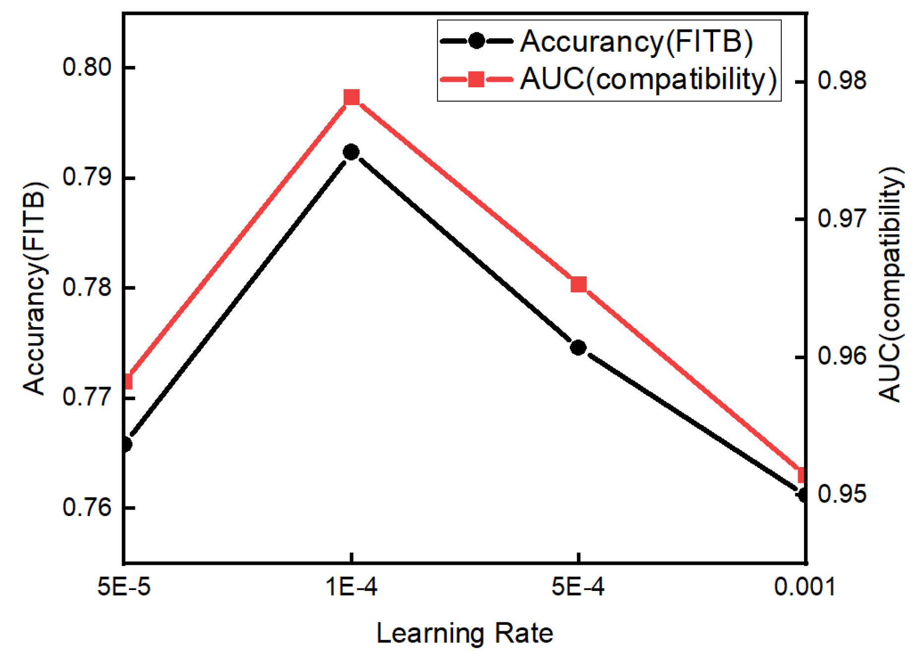
5.6.3. Effect of the Learning Rate

To investigate whether the learning rate had an effect on model performance by changing the size of learning rate, we search the layers in the range of $\{0.001,0.0005,0.0001,0.00005\}$ in particular. We show the results in Figure 9. The performance was optimal when the learning rate was 0.0001. The results show that the learning rate cannot be set too high or too low. Too high a rate will cause the model to fail to converge, while too low a rate will cause the model to converge very slowly and even reach a local extreme point.

6. Conclusions

In this work, we incorporated a hypergraph explicitly into the overall compatibility prediction of outfits. The hyperedge in the hypergraph can represent an outfit completely, and the complex relationships between different items in the outfit can be better captured by transforming the hyperedge into a simple graph. In order to better infer whether the outfit is compatible from the hypergraph, we propose a new framework OCPHN to solve the problem of outfit compatibility modeling. The model can better model complex interactions between nodes and learn better node representations. We conducted experiments on different types of fashion-matching tasks using a real-world dataset (Polyvore dataset), and the results demonstrate that our model can learn the compatibility of fashion outfits effectively and outperform the state-of-the-art methods. Since fashion compatibility is a complex task and might vary from one person to another, modeling user-specific compatibility and style preferences is one of our future research directions.

References

1. Kang, W.C.; Fang, C.; Wang, Z.; McAuley, J. Visually-Aware Fashion Recommendation and Design with Generative Image Models. In Proceedings of the 2017 IEEE International Conference on Data Mining (ICDM), New Orleans, LA, USA, 18–21 November 2017. [Google Scholar]
2. Feng, Z.; Yu, Z.; Yang, Y.; Jing, Y.; Jiang, J.; Song, M. Interpretable Partitioned Embedding for Customized Multi-item Fashion Outfit Composition. In Proceedings of the 2018 ACM on International Conference on Multimedia Retrieval, Yokohama, Japan, 11–14 June 2018. [Google Scholar]
3. Hsiao, W.L.; Grauman, K. Creating Capsule Wardrobes from Fashion Images. In Proceedings of the IEEE Conference on Computer Vision and Pattern Recognition (CVPR), Salt Lake City, UT, USA, 18–23 June 2018. [Google Scholar]
4. Gu, X.; Wong, Y.; Shou, L.; Peng, P.; Chen, G.; Kankanhalli, M.S. Multi-Modal and Multi-Domain Embedding Learning for Fashion Retrieval and Analysis. IEEE Trans. Multimed. 2019, 21, 1524–1537. [Google Scholar] [CrossRef]
5. Jiang, H.; Wang, W.; Wei, Y.; Gao, Z.; Wang, Y.; Nie, L. What Aspect Do You Like: Multi-scale Time-aware User Interest Modeling for Micro-video Recommendation. In Proceedings of the 28th ACM International Conference on Multimedia, Seattle, WA, USA, 12–16 October 2020. [Google Scholar]
6. Yu, X.; Gan, T.; Wei, Y.; Cheng, Z.; Nie, L. Personalized Item Recommendation for Second-hand Trading Platform. In Proceedings of the 28th ACM International Conference on Multimedia, Seattle, WA, USA, 12–16 October 2020. [Google Scholar]
7. Al-Halah, Z.; Stiefelhagen, R.; Grauman, K. Fashion Forward: Forecasting Visual Style in Fashion. In Proceedings of the IEEE International Conference on Computer Vision (ICCV), Venice, Italy, 22–29 October 2017. [Google Scholar]
8. Zhan, H.; Lin, J.; Ak, K.E.; Shi, B.; Duan, L.Y.; Kot, A.C. A3-FKG: Attentive Attribute-Aware Fashion Knowledge Graph for Outfit Preference Prediction. IEEE Trans. Multimed. 2021, 24, 819–831. [Google Scholar] [CrossRef]
9. Vasileva, M.I.; Plummer, B.A.; Dusad, K.; Rajpal, S.; Kumar, R.; Forsyth, D. Learning Type-Aware Embeddings for Fashion Compatibility. In Proceedings of the European Conference on Computer Vision (ECCV), Munich, Germany, 8–14 September 2018. [Google Scholar]
10. Bell, S.; Bala, K. Learning Visual Similarity for Product Design with Convolutional Neural Networks. ACM Trans. Graph. 2015, 34, 1–10. [Google Scholar] [CrossRef]
11. Song, X.; Feng, F.; Han, X.; Yang, X.; Liu, W.; Nie, L. Neural Compatibility Modeling with Attentive Knowledge Distillation. In Proceedings of the 41st International ACM SIGIR Conference on Research and Development in Information Retrieval, Ann Arbor, MI, USA, 8–12 July 2018. [Google Scholar]
12. Jing, P.; Zhang, J.; Nie, L.; Ye, S.; Liu, J.; Su, Y. Tripartite Graph Regularized Latent Low-Rank Representation for Fashion Compatibility Prediction. IEEE Trans. Multimed. 2021, 24, 1277–1287. [Google Scholar] [CrossRef]
13. Song, X.; Fang, S.T.; Chen, X.; Wei, Y.; Zhao, Z.; Nie, L. Modality-Oriented Graph Learning Toward Outfit Compatibility Modeling. IEEE Trans. Multimed. 2021. [Google Scholar] [CrossRef]
14. Jing, P.; Ye, S.; Nie, L.; Liu, J.; Su, Y. Low-Rank Regularized Multi-Representation Learning for Fashion Compatibility Prediction. IEEE Trans. Multimed. 2020, 22, 1555–1566. [Google Scholar] [CrossRef]
15. McAuley, J.; Targett, C.; Shi, Q.; Van Den Hengel, A. Image-Based Recommendations on Styles and Substitutes. In Proceedings of the 38th International ACM SIGIR Conference on Research and Development in Information Retrieval, Santiago, Chile, 9–13 August 2015. [Google Scholar]
16. Veit, A.; Kovacs, B.; Bell, S.; McAuley, J.; Bala, K.; Belongie, S. Learning Visual Clothing Style with Heterogeneous Dyadic Co-Occurrences. In Proceedings of the IEEE International Conference on Computer Vision (ICCV), Santiago, Chile, 7–13 December 2015. [Google Scholar]
17. Han, X.; Song, X.; Yin, J.; Wang, Y.; Nie, L. Prototype-guided Attribute-wise Interpretable Scheme for Clothing Matching. In Proceedings of the 42nd International ACM SIGIR Conference on Research and Development in Information Retrieval, Paris, France, 21–25 July 2019. [Google Scholar]
18. Shih, Y.S.; Chang, K.Y.; Lin, H.T.; Sun, M. Compatibility Family Learning for Item Recommendation and Generation. In Proceedings of the AAAI Conference on Artificial Intelligence, New Orleans, LA, USA, 2–7 February 2018. [Google Scholar]
19. He, R.; Packer, C.; McAuley, J. Learning Compatibility Across Categories for Heterogeneous Item Recommendation. In Proceedings of the IEEE 16th International Conference on Data Mining (ICDM), Barcelona, Spain, 12–15 December 2016. [Google Scholar]
20. Li, Y.; Cao, L.; Zhu, J.; Luo, J. Mining Fashion Outfit Composition Using an End-to-End Deep Learning Approach on Set Data. IEEE Trans. Multimed. 2017, 19, 1946–1955. [Google Scholar] [CrossRef] [Green Version]
21. Song, X.; Feng, F.; Liu, J.; Li, Z.; Nie, L.; Ma, J. NeuroStylist: Neural Compatibility Modeling for Clothing Matching. In Proceedings of the 25th ACM International Conference on Multimedia, Mountain View, CA, USA, 23–27 October 2017. [Google Scholar]
22. Han, X.; Wu, Z.; Jiang, Y.G.; Davis, L.S. Learning Fashion Compatibility with Bidirectional LSTMs. In Proceedings of the 25th ACM International Conference on Multimedia, Mountain View, CA, USA, 23–27 October 2017. [Google Scholar]
23. Nakamura, T.; Goto, R. Outfit Generation and Style Extraction via Bidirectional LSTM and Autoencoder. In Proceedings of the KDD Workshop AI for fashion, London, UK, 20–25 August 2018. [Google Scholar]
24. Veit, A.; Belongie, S.J.; Karaletsos, T. Conditional Similarity Networks. In Proceedings of the IEEE Conference on Computer Vision and Pattern Recognition (CVPR), Honolulu, HI, USA, 21–26 July 2017. [Google Scholar]
25. Cui, Z.; Li, Z.; Wu, S.; Zhang, X.Y.; Wang, L. Dressing as a Whole: Outfit Compatibility Learning Based on Node-Wise Graph Neural Networks. In Proceedings of the World Wide Web Conference, San Francisco, CA, USA, 13–17 May 2019. [Google Scholar]
26. Cucurull, G.; Taslakian, P.; Vazquez, D. Context-Aware Visual Compatibility Prediction. In Proceedings of the IEEE/CVF Conference on Computer Vision and Pattern Recognition (CVPR), Long Beach, CA, USA, 15–20 June 2019. [Google Scholar]
27. Wei, Y.; Wang, X.; Nie, L.; He, X.; Hong, R.; Chua, T.S. MMGCN: Multi-Modal Graph Convolution Network for Personalized Recommendation of Micro-Video. In Proceedings of the 27th ACM International Conference on Multimedia, Nice, France, 21–25 October 2019. [Google Scholar]
28. Tao, Z.; Wei, Y.; Wang, X.; He, X.; Huang, X.; Chua, T.S. MGAT: Multimodal Graph Attention Network for Recommendation. Inf. Process. Manag. 2020, 57, 102277. [Google Scholar] [CrossRef]
29. Wei, Y.; Wang, X.; Nie, L.; He, X.; Chua, T.S. Graph-refined Convolutional Network for Multimedia Recommendation with Implicit Feedback. In Proceedings of the 28th ACM International Conference on Multimedia, Seattle, WA, USA, 12–16 October 2020. [Google Scholar]
30. Gori, M.; Monfardini, G.; Scarselli, F. A New Model for Learning in Graph Domains. In Proceedings of the International Joint Conference on Neural Networks, Montreal, QC, Canada, 31 July–4 August 2005. [Google Scholar]
31. Scarselli, F.; Gori, M.; Tsoi, A.C.; Hagenbuchner, M.; Monfardini, G. The Graph Neural Network Model. IEEE Trans. Neural Networks 2009, 20, 61–80. [Google Scholar] [CrossRef] [PubMed] [Green Version]
32. Gallicchio, C.; Micheli, A. Graph Echo State Networks. In Proceedings of the 2010 International Joint Conference on Neural Networks (IJCNN), Barcelona, Spain, 18–23 July 2010. [Google Scholar]
33. Li, Y.; Tarlow, D.; Brockschmidt, M.; Zemel, R. Gated Graph Sequence Neural Networks. In Proceedings of the International Conference on Learning Representations, Caribe Hilton. San Juan, Puerto Rico, 2–4 May 2016. [Google Scholar]
34. Kipf, T.N.; Welling, M. Semi-Supervised Classification with Graph Convolutional Networks. In Proceedings of the International Conference on Learning Representations, Toulon, France, 24–26 April 2017. [Google Scholar]
35. Hamilton, W.; Ying, Z.; Leskovec, J. Inductive Representation Learning on Large Graphs. In Proceedings of the Advances in Neural Information Processing Systems, Long Beach, CA, USA, 4–9 December 2017. [Google Scholar]
36. Veličković, P.; Cucurull, G.; Casanova, A.; Romero, A.; Liò, P.; Bengio, Y. Graph Attention Networks. In Proceedings of the International Conference on Learning Representations, Vancouver, BC, Canada, 30 April–3 May 2018. [Google Scholar]
37. Zhou, D.; Huang, J.; Schölkopf, B. Learning with Hypergraphs: Clustering, Classification, and Embedding. In Proceedings of the Advances in Neural Information Processing Systems, Vancouver, BC, Canada, 4–9 December 2006. [Google Scholar]
38. Feng, Y.; You, H.; Zhang, Z.; Ji, R.; Gao, Y. Hypergraph Neural Networks. In Proceedings of the AAAI Conference on Artificial Intelligence, Honolulu, HI, USA, 27 January–1 February 2019. [Google Scholar]
39. Yadati, N.; Nimishakavi, M.; Yadav, P.; Nitin, V.; Louis, A.; Talukdar, P. HyperGCN: A New Method for Training Graph Convolutional Networks on Hypergraphs. In Proceedings of the Advances in Neural Information Processing Systems, Vancouver, BC, Canada, 8–14 December 2019. [Google Scholar]
40. Jiang, J.; Wei, Y.; Feng, Y.; Cao, J.; Gao, Y. Dynamic Hypergraph Neural Networks. In Proceedings of the 28th International Joint Conference on Artificial Intelligence, Macao, China, 10–16 August 2019. [Google Scholar]
41. Tu, K.; Cui, P.; Wang, X.; Wang, F.; Zhu, W. Structural Deep Embedding for Hyper-Networks. In Proceedings of the AAAI Conference on Artificial Intelligence, New Orleans, LA, USA, 2–7 February 2018. [Google Scholar]
42. Zhang, R.; Zou, Y.; Ma, J. Hyper-SAGNN: A Self-attention Based Graph Neural Network for Hypergraphs. In Proceedings of the International Conference on Learning Representations, Addis Ababa, Ethiopia, 26 April–1 May 2020. [Google Scholar]
43. Donahue, J.; Jia, Y.; Vinyals, O.; Hoffman, J.; Zhang, N.; Tzeng, E.; Darrell, T. DeCAF: A Deep Convolutional Activation Feature for Generic Visual Recognition. In Proceedings of the 31st International Conference on Machine Learning, Bejing, China, 22–24 June 2014. [Google Scholar]
44. Sharif Razavian, A.; Azizpour, H.; Sullivan, J.; Carlsson, S. CNN Features Off-the-Shelf: An Astounding Baseline for Recognition. In Proceedings of the IEEE Conference on Computer Vision and Pattern Recognition (CVPR) Workshops, Columbus, OH, USA, 23–28 June 2014. [Google Scholar]
45. Maas, A.L.; Hannun, A.Y.; Ng, A.Y. Rectifier Nonlinearities Improve Neural Network Acoustic Models. In Proceedings of the 30th International Conference on Machine Learning, Atlanta, GA, USA, 16–21 June 2013. [Google Scholar]
46. Rendle, S.; Freudenthaler, C.; Gantner, Z.; Schmidt-Thieme, L. BPR: Bayesian Personalized Ranking from Implicit Feedback. In Proceedings of the 25th Conference on Uncertainty in Artificial Intelligence, Montreal, QC, Canada, 19–21 June 2009. [Google Scholar]
47. Wei, Y.; Wang, X.; Li, Q.; Nie, L.; Li, Y.; Li, X.; Chua, T.S. Contrastive Learning for Cold-Start Recommendation. In Proceedings of the 29th ACM International Conference on Multimedia, Virtual Event, China, 20–24 October 2021. [Google Scholar]
48. Wei, Y.; Wang, X.; He, X.; Nie, L.; Rui, Y.; Chua, T.S. Hierarchical User Intent Graph Network for Multimedia Recommendation. IEEE Trans. Multimed. 2022, 24, 2701–2712. [Google Scholar] [CrossRef]
Figure 1. Example compatible and incompatible outfits.
Mathematics 10 03913 g001
Figure 2. Overview of the proposed method. Based on the dataset, we first construct a fashion hypergraph, where an outfit (e.g., coats, short sleeves, handbags, high heels and skirts) can be represented as a hyperedge. We then design OCPHN to better model the node interactions in a hyperedge and refine the node representations. Finally, the compatibility score is calculated by the attention mechanism to predict the outfit compatibility.
Mathematics 10 03913 g002
Figure 3. An illustration of the fashion hypergraph based on the dataset, where each circle indicates a category and each hyperedge represents the matching interactions between multiple categories (i.e., they appear in an identical outfit).
Mathematics 10 03913 g003
Figure 4. An illustration of transforming the hyperedge into a simple graph, where the key nodes e i and e j (i.e., the two nodes with the greatest difference) are selected from the hyperedge, and the remaining nodes e k in the hyperedge are connected with the key nodes to form a new simple graph.
Mathematics 10 03913 g004
Figure 5. Comparison of our model and two baselines (i.e., NGNN and Bi-LSTM) for fill-in-the-blank task. Green font represents the right answer, and red font represents the wrong answer.
Mathematics 10 03913 g005
Figure 6. Results of our method in the fashion outfit compatibility prediction task. To be more intuitive, scores are normalized to be between 0 and 1.
Mathematics 10 03913 g006
Figure 7. Test performance in different dimensions.
Mathematics 10 03913 g007
Figure 8. Test performance in different propagation layers.
Mathematics 10 03913 g008
Figure 9. Test performance at different learning rates.
Mathematics 10 03913 g009