Trajectory Tracking Design for a Swarm of Autonomous Mobile Robots: A Nonlinear Adaptive Optimal Approach

Abstract

This research presents a nonlinear adaptive optimal control approach to the trajectory tracking problem of a swarm of autonomous mobile robots. Mathematically, finding an analytical adaptive control solution that meets the H₂ performance index for the trajectory tracking problem when controlling a swarm of autonomous mobile robots is an almost impossible task, due to the great complexity and high dimensions of the dynamics. For deriving an analytical adaptive control law for this tracking problem, a particular formulation for the trajectory tracking error dynamics between a swarm of autonomous mobile robots and the desired trajectory is made via a filter link. Based on this prior analysis of the trajectory tracking error dynamics, a closed-form adaptive control law is analytically derived from a high-dimensional nonlinear partial differential equation, which is equivalent to solving the trajectory tracking problem of a swarm of autonomous mobile robots with respect to an H₂ performance index. This delivered adaptive nonlinear control solution offers the advantages of a simple control structure and good energy-saving performance. From the trajectory tracking verification, this proposed control approach possesses satisfactory trajectory tracking performance for a swarm of autonomous mobile robots, even under the effects of huge modeling uncertainties.

1. Introduction

In recent decades, the diverse applications of autonomous mobile robots (AMRs) have attracted much attention. Individually developed AMRs offer solutions for transportation, security, inspection, and so on. Until now, most published studies, including backstepping control [1,2,3,4], sliding mode control [5,6,7,8], feedback linearization control [9,10,11], neural network control [12,13,14,15], and fuzzy control [16,17,18,19,20,21,22] have focused on the trajectory tracking design of a single AMR. In practice, these proposed control designs are complicated in practice and usually demand higher computational consumption. For achieving the abovementioned real applications, AMRs with long energy endurance, high maneuverability, and tracking ability are required. Thus, effective optimal control, along with energy-saving capacity, is important for AMRs, and several related publications [23,24,25,26,27,28,29,30] will be discussed. Two main methods could allow AMRs to present good energy-saving performance. The first one is a lower usage of driven actuators, such as motors, and the second is that a simple optimal control structure should be developed. The first issue can be solved by utilizing a mobile robot with a configuration that has two active wheels and one passive wheel. The only way to address the second issue is a closed-form solution or analytical solution that can be derived for the optimal trajectory tracking problem of AMRs. The analytical design for the optimal control of a single AMR was developed by the authors of [31], based on the coordinate transformation. However, the complexity of the overall dynamic is highly increased when a swarm of AMRs needs to be controlled simultaneously. The solvability of the optimal trajectory tracking problem of a swarm of AMRs degrades to almost zero; mathematically deriving the analytical solution for tracking the trajectory of a swarm of AMRs is a difficult task. To the best of the authors’ knowledge, an optimal control design for the trajectory tracking of a swarm of AMRs is rare. By careful arrangement, an analytical solution was delivered to achieve the optimal trajectory tracking of a swarm of AMRs in [32]. This developed result provides a low energy consumption solution for the trajectory tracking problem of a swarm of AMRs with stationary system parameters. In practice, AMRs with fixed system parameters are particular cases, and system parameters such as mass, inertia, etc., inevitably change due to the variations in payload and energy loss. Hence, for compensating the issue of system parameter variations that are never considered in the optimal control design process of [32], an innovative nonlinear adaptive optimal control approach that offers a closed-form design with an easy-to-implement control structure and precise trajectory tracking performance is proposed. This offers an optimal trajectory tracking solution for the problem of a swarm of AMRs with modeling uncertainties in this investigation. For tackling the varying system parameters of a swarm of AMRs, a parameterized formulation is used on-line to precisely estimate the time-varying system parameters, including mass, inertia, and so on. Furthermore, an adaptive control law that contains this parameter estimation term is developed analytically to satisfy an H₂ performance index corresponding to the optimal trajectory tracking problem of a swarm of AMRs with modeling uncertainties. This proposed adaptive control law offers good energy-saving performance because it is a closed-form solution and can mitigate the effect of varying modeling uncertainties. This research is presented as follows: the introduction and a literature review are given in Section 1; a description of the tracking error dynamics between a swarm of AMRs and the desired trajectory is given in Section 2; statements regarding the proposed adaptive H₂ closed-form control law are expressed in Section 3; the simulation results for a swarm of AMRs based on this proposed approach are illustrated in Section 4; Section 5 summarizes our conclusions from this investigation.

2. Trajectory Tracking Dynamics for a Swarm of Autonomous Mobile Robots

The trajectory tracking dynamics of a swarm of AMRs that integrates n AMRs is briefly described in this section. Furthermore, the nonlinear trajectory tracking error dynamics between a swarm of AMRs and the desired trajectory, in terms of global coordinates, is formulated.

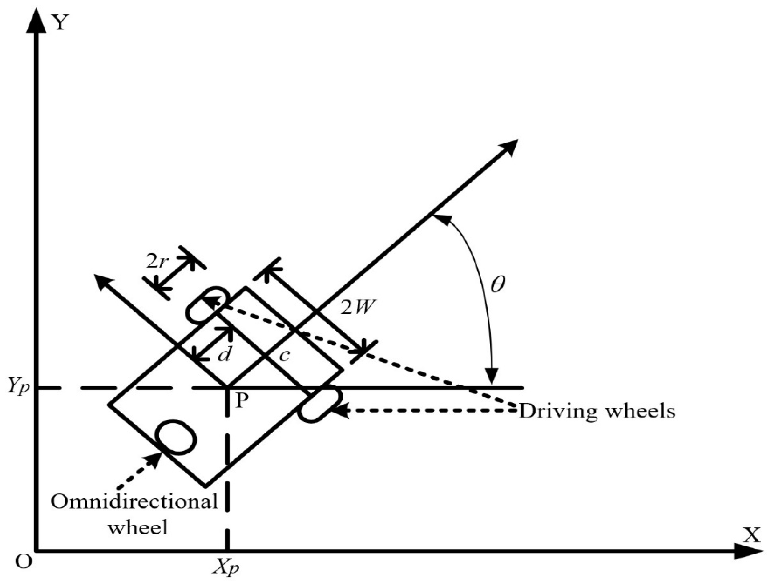
2.1. Dynamics of a Single AMR

From the schematics of the single AMR in Figure 1, it is easy to find out that this AMR is separated by 2W; two driving wheels have the same radius of r in the heading direction and an omnidirectional wheel is installed in the back. The instantaneous position of this controllable AMR in the Earth frame {O, X, Y} is denoted as c. P = ($x_p$,$y_p$) represents the position of the controllable AMR in the Earth frame, and the angle θ denotes the direction of the Body frame {P, X_p, Y_p}. According to the aforementioned descriptions, the universal coordinate frame of the AMR can be presented using Equation (1), as follows:

$$c={[\begin{array}{ccc}{x}_p& y_p& \theta \end{array}]}^T$$

(1)

The AMR illustrated in Figure 1 usually moves along the orientation of the axis of the driving wheels, and the kinematics of the AMR with constraints can be described as follows [33]:

$$\dot{c}=\left[\begin{array}{c}{\dot{x}}_p\\ {\dot{y}}_p\\ \dot{\theta }\end{array}\right]=\left[\begin{array}{cc}\cos \theta & -d\sin \theta \\ \sin \theta & d\cos \theta \\ 0& 1\end{array}\right]\left[\begin{array}{c}{v}_l\\ \omega \end{array}\right]$$

(2)

where $v_l$ and $\omega$ denote the linear and angular velocities, respectively.

Based on the AMR kinematics in Equation (2), and since n AMRs are supposed to be considered in this investigation, the dynamics of each single AMR can be inferred, as in Equation (3):

$$F_i(c_i){\ddot{c}}_i+O_i(c_i,{\dot{c}}_i){\dot{c}}_i+G_i(c_i)=M_i(c_i){\tau }_i,\text{ for }i=1,\dots ,n$$

(3)

where $F_i(c_i)\in {\Re }^{3\times 3}$ is a symmetric positive definite inertia matrix, $O_i(c_i,{\dot{c}}_i)\in {\Re }^{3\times 3}$ denotes the Coriolis and centripetal force matrix, $G_i(c_i)\in {\Re }^{3\times 3}$ denotes the gravitational vector, $M_i(c_i)\in {\Re }^{3\times 2}$ denotes the transformation matrix, and ${\tau }_i\in {\Re }^{2\times 1}$ is the torque vector and can be regarded as the control input vector. As to ${\dot{c}}_i$ and ${\ddot{c}}_i$, they are the velocity and acceleration vectors of the controlled AMR, with the index, i. Practically speaking, the gravitational vector $G_i(c_i)$ is countervailed naturally, due to the reaction force from the ground to the controlled AMR. This term can be ignored from the dynamics in Equation (3).

The modified dynamics of the controlled AMR can be further described as the following:

$$F_i(c_i){\ddot{c}}_i+O_i(c_i,{\dot{c}}_i){\dot{c}}_i=M_i(c_i){\tau }_i,\text{ for }i=1,\dots ,n.$$

(4)

Details of $F_i(c_i)\in {\Re }^{3\times 3}$, $O_i(c_i,{\dot{c}}_i)$ and $M_i(c_i)\in {\Re }^{3\times 2}$ are given below:

$$F_i(c_i)=\left[\begin{array}{ccc}{m}_i& 0& m_i{d}_i\sin {\theta }_i\\ 0& m_i& -m_i{d}_i\cos {\theta }_i\\ m_i{d}_i\sin {\theta }_i& -m_i{d}_i\cos {\theta }_i& I_{Pi}\end{array}\right]$$

(5)

$$O_i(c_i,{\ddot{c}}_i)=\left[\begin{array}{ccc}0& 0& m_i{d}_i{\dot{\theta }}_i\cos {\theta }_i\\ 0& 0& m_i{d}_i{\dot{\theta }}_i\sin {\theta }_i\\ 0& 0& 0\end{array}\right]$$

(6)

$$M_i(c_i)=\frac{1}{r_i}\left[\begin{array}{cc}\cos {\theta }_i& \sin {\theta }_i\\ \sin {\theta }_i& \sin {\theta }_i\\ W_i& -W_i\end{array}\right]$$

(7)

$${\tau }_i=\left[\begin{array}{c}{\tau }_{ri}\\ {\tau }_{li}\end{array}\right]$$

(8)

where ${\tau }_{ri}$ and ${\tau }_{li}$ are the right and left wheel torques, respectively, $m_i$ stands for the mass, $d_i$ is the distance between P and c, $I_{Pi}$ is the inertia, and ${\theta }_i$ is the heading angle. In this investigation, the system parameters ($m_i$, $d_i$, $I_{Pi}$) are uncertain due to modeling perturbations representing variations in payloads $\Delta m_i$.

2.2. Trajectory Tracking Error Dynamics

We assume that the related desired trajectory $c_{ri}$ used in this investigation is a twice continuously differentiable function $c_{ri}\in C^2$ and denote ${\dot{c}}_{ri}$ and ${\ddot{c}}_{ri}$ as the velocity and acceleration vector of the $c_{ri}$, respectively. According to the above statement, the trajectory tracking error between the controlled AMR $c_i$ and the related desired trajectory $c_{ri}$ can be expressed as follows:

$$e=\left[\begin{array}{c}{\dot{\widehat{c}}}_i\\ {\widehat{c}}_i\end{array}\right]=\left[\begin{array}{c}{\dot{c}}_i-{\dot{c}}_{ri}\\ c_i-c_{ri}\end{array}\right]$$

(9)

where:

$$c_{ri}={[{\begin{array}{ccc}{x}_{di}& y_{di}& \theta \end{array}}_{di}]}^T$$

(10)

The dynamics of the trajectory tracking error can be easily derived using Equations (4) and (9), as below:

$${\dot{e}}_i=\left[\begin{array}{cc}-F_i{}^{-1}(c_i)O_i(c_i,{\dot{c}}_i)& 0_{3\times 3}\\ I_{3\times 3}& 0_{3\times 3}\end{array}\right]e_i+\left[\begin{array}{c}-{\ddot{c}}_{ri}-F_i{}^{-1}(c_i)O_i(c_i,{\dot{c}}_i){\dot{c}}_{ri}\\ 0_{3\times 3}\end{array}\right]+\left[\begin{array}{c}{F}_i{}^{-1}(c_i)M_i(c_i){\tau }_i\\ 0_{3\times 3}\end{array}\right]$$

(11)

By observing the governing equations of the controlled AMR in Equation (11), we found that it is difficult to treat this trajectory tracking problem involving a swarm of AMRs with Equation (11), if the design target is to find out the analytical solution to this problem. For solving this issue, the following mapping of $l_i(t)$ is constructed:

$$l_i(t)={\delta }_i{\dot{\widehat{c}}}_i+{\epsilon }_i{\widehat{c}}_i$$

(12)

where ${\delta }_i$ and ${\epsilon }_i$ are designable positive constants.

The differentiation of the mapping $l_i(t)$ is:

$${\dot{l}}_i(t)=-F_i{}^{-1}(c_i)O_i(c_i,{\dot{c}}_i)l_i(t)+{\epsilon }_i{F}_i{}^{-1}(c_i)\left[-{\mathsf{\Phi }}_i(t){\xi }_i(t)+M_i(c_i){\tau }_i\right]$$

(13)

where:

$${\mathsf{\Phi }}_i(t){\xi }_i(t)={\mathsf{\Phi }}_i(c_i,{\dot{c}}_i,{\dot{c}}_{ir}-\frac{{\delta }_i}{{\epsilon }_i}{\widehat{c}}_i,{\ddot{c}}_{ir}-\frac{{\delta }_i}{{\epsilon }_i}{\dot{\widehat{c}}}_i){\xi }_i(t)=F_i(c_i)({\ddot{c}}_{ir}-\frac{{\delta }_i}{{\epsilon }_i}{\dot{\widehat{c}}}_i)+O_i(c_i,{\dot{c}}_i)({\dot{c}}_{ir}-\frac{{\delta }_i}{{\epsilon }_i}{\widehat{c}}_i)$$

(14)

$${\mathsf{\Phi }}_i(t)=\left[\begin{array}{ccc}{\ddot{x}}_i& {\dot{y}}_i\sin {\theta }_i+{\dot{\theta }}_i{}^2\cos {\theta }_i& 0\\ {\ddot{y}}_i& -{\dot{\theta }}_i\cos {\theta }_i+{\dot{\theta }}_i{}^2\sin {\theta }_i& 0\\ 0& {\ddot{x}}_i\sin {\theta }_i-{\ddot{y}}_i\cos {\theta }_i& {\ddot{\theta }}_i\end{array}\right]$$

(15)

$${\xi }_i(t)=\left[\begin{array}{c}{m}_i\\ m_i{d}_i\\ I_{pi}\end{array}\right]$$

(16)

By using Equation (13), the trajectory tracking error dynamics in Equation (11) can be revised as a formulation with a parameterized term ${\mathsf{\Phi }}_i(t){\xi }_i(t)$ for the purpose of precisely estimating the disturbed systems’ parameters, $m_i$, $d_i$ and $I_{pi}$:

$${\dot{e}}_i=T^{-1}\left[\begin{array}{c}{\dot{l}}_i(t)\\ {\dot{\widehat{c}}}_i(t)\end{array}\right]=H_i(e_i,t)e_i(t)+{\epsilon }_i{P}_i(e_i,t)\left[-{\mathsf{\Phi }}_i(t){\xi }_i(t)+{\tau }_i{}^{\prime }\right]$$

(17)

in which:

$$H_i(e_i,t)=T_i{}^{-1}\left[\begin{array}{cc}-F_i{}^{-1}(c_i)O_i(c_i,{\dot{c}}_i)& 0_{3\times 3}\\ \frac{1}{{\epsilon }_i}{I}_{3\times 3}& -\frac{{\delta }_i}{{\epsilon }_i}{I}_{3\times 3}\end{array}\right]T_i$$

(18)

$$P_i(e_i,t)=T_i{}^{-1}{B}_i{F}_i{}^{-1}(c_i)$$

(19)

$$B_i=\left[\begin{array}{c}{I}_{3\times 3}\\ 0_{3\times 3}\end{array}\right]$$

(20)

$${\tau }_i{}^{\prime }=M_i(c_i){\tau }_i$$

(21)

and $T_i$ is the state-space transformation matrix:

$$T_i=\left[\begin{array}{cc}{\delta }_i{I}_{3\times 3}& {\epsilon }_i{I}_{3\times 3}\\ I_{3\times 3}& 0_{3\times 3}\end{array}\right]$$

(22)

whence ${\delta }_i$ and ${\epsilon }_i$ will be derived in the following section.

If we choose ${\tau }_i{}^{\prime }$ as:

$${\tau }_i{}^{\prime }={\mathsf{\Phi }}_i(t){\widehat{\xi }}_i(t)+\frac{1}{{\epsilon }_i}{u}_i$$

(23)

Then modified trajectory tracking error dynamics for each AMR of a swarm of AMRs can be further presented as:

$${\dot{e}}_i=H_i(e_i,t)e_i(t)+P_i(e_i,t)\left[{\epsilon }_i{\mathsf{\Phi }}_i(t){\tilde{\xi }}_i(t)+u_i\right]$$

(24)

where ${\tilde{\xi }}_i(t)={\widehat{\xi }}_i(t)-{\xi }_i(t)$ denotes the parameter estimation errors.

The overall trajectory tracking error dynamics of a swarm of AMRs can be further described using the following vector-matrix form:

$$\dot{E}(t)=H(E(t),t)E(t)+P(E(t),t)\epsilon \mathsf{\Phi }(t)\tilde{\xi }(t)+P(E(t),t)U(t)$$

(25)

where:

$$E(t)={\left[\begin{array}{ccccc}{e}_1(t)& e_2(t)& \dots & e_{n-1}(t)& e_n(t)\end{array}\right]}^T$$

(26)

$$H(E(t),t)=diag\left(H_1(e_1,t),H_2(e_2,t),\dots ,H_n(e_n,t)\right)$$

(27)

$$P(E(t),t)=diag\left(P_1(e_1,t),P_2(e_2,t),\dots ,P_n(e_n,t)\right)$$

(28)

$$\epsilon ={\left[\begin{array}{ccccc}{\epsilon }_1& {\epsilon }_2& \dots & {\epsilon }_{n-1}& {\epsilon }_n\end{array}\right]}^T$$

(29)

$$\mathsf{\Phi }(t)=diag\left({\mathsf{\Phi }}_1(t),{\mathsf{\Phi }}_2(t),\dots ,{\mathsf{\Phi }}_n(t)\right)$$

(30)

$$\tilde{\xi }(t)=diag\left({\tilde{\xi }}_1(t),{\tilde{\xi }}_2(t),\dots ,{\tilde{\xi }}_n(t)\right)$$

(31)

$$U(t)={\left[\begin{array}{ccccc}{u}_1& u_2& \dots & u_{n-1}& u_n\end{array}\right]}^T$$

(32)

3. Nonlinear Adaptive Optimal Control Approach

3.1. The Trajectory Tracking Problem of a Swarm of AMRs

When we consider the overall trajectory tracking error dynamics of a swarm of AMRs in Equation (25), the design objective is to develop an adaptive H₂ closed-form control law to satisfy the H₂ performance index. The trajectory tracking problem of a swarm of AMRs is solved if this problem exists when a closed-form solution $U^{*}(t)$ and an adaptive law $\widehat{\xi }(t)$ can fulfill the H₂ optimal performance index, below, for all $t_f\in [0,\infty )$:

$$\begin{array}{l}\Gamma (U^{*})=\underset{U\left(t\right)\in \left[0,t_f\right)}{\min }\left[E^T(t_f)K_{f}E(t_f)+{\tilde{\xi }}^T(t_f)R\tilde{\xi }(t_f)+{\displaystyle {\int }_0^{t_f}\left[E^T(t)KE(t)+U^T(t)SU(t)\right]}dt\right]\\ =E^T(0)\Gamma (E(0),0)E(0)+{\tilde{\xi }}^T(0)R\tilde{\xi }(0)\end{array}$$

(33)

where $K_f=diag\left(K_{f1},K_{f2},\dots ,K_{fn}\right)$, $K=diag\left(K_1,K_2,\dots ,K_n\right)$, $R=diag\left(R_1,R_2,\dots ,R_n\right)$ and $S=diag\left(S_1,S_2,\dots ,S_n\right)$ are the designated positive definite weighted matrices, $K_f=K_f^T$, and $S=S^T>0$.

Based on the mathematical proof shown in Appendix A, if one unique solution $\Gamma (E(t),t)$ can be found for the following nonlinear and time-varying differential equation, the trajectory tracking problem of a swarm of AMRs is guaranteed to be solved analytically. In this instance:

$$\begin{array}{l}\dot{\Gamma }(E(t),t)+\Gamma (E(t),t)H(E(t),t)+H^T(E(t),t)\Gamma (E(t),t)+K\\ -\Gamma (E(t),t)P(E(t),t)S^{-1}{P}^T(E(t),t)\Gamma (E(t),t)=0\end{array}$$

(34)

and the corresponding control law can be described as:

$${\tau }^{\prime }(E(t),t)=\mathsf{\Phi }(t)\widehat{\xi }(t)+\frac{1}{\epsilon }{U}^{*}(E(t),t)$$

(35)

where:

$$U^{*}(E(t),t)=-S^{-1}{P}^T(E(t),t)\Gamma (E(t),t)E(t)$$

(36)

$$\dot{\widehat{\xi }}(t)=-\epsilon R^{-1}{\mathsf{\Phi }}^T(t)P^T(E(t),t)\Gamma (E(t),t)E(t)$$

(37)

$$\Gamma (E(t),t)={\Gamma }^T(E(t),t)\ge 0$$

(38)

The details of Equation (34) are revealed below:

$$\left[\begin{array}{c}{\dot{\Gamma }}_1(e_1,t)+{\Gamma }_1(e_1,t)H_1(e_1,t)+H_1^T(e_1,t){\Gamma }_1(e_1,t)+K_1-{\Gamma }_1(e_1,t)P_1(e_1,t)S_1^{-1}{P}_1^T(e_1,t){\Gamma }_1(e_1,t)\\ {\dot{\Gamma }}_2(e_2,t)+{\Gamma }_2(e_2,t)H_2(e_2,t)+H_2^T(e_2,t){\Gamma }_2(e_2,t)+K_2-{\Gamma }_2(e_2,t)P_2(e_2,t)S_2^{-1}{P}_2^T(e_2,t){\Gamma }_2(e_2,t)\\ ⋮\\ ⋮\\ ⋮\\ {\dot{\Gamma }}_n(e_n,t)+{\Gamma }_n(e_n,t)H_n(e_n,t)+H_n^T(e_n,t){\Gamma }_n(e_n,t)+K_n-{\Gamma }_n(e_n,t)P_n(e_n,t)S_n^{-1}{P}_n^T(e_n,t){\Gamma }_n(e_n,t)\end{array}\right]=\left[\begin{array}{c}0\\ 0\\ ⋮\\ ⋮\\ ⋮\\ 0\end{array}\right]$$

(39)

Then, the trajectory tracking problem of a swarm of AMRs is likewise solved.

3.2. Analytical Solution $\Gamma (E(t),t)$ of the Trajectory Tracking Problem of a Swarm of AMRs

By observing Equation (34), it is obvious that the trajectory tracking problem is analytically solved if the closed-form solution $\Gamma (E(t),t)$, i.e., ${\Gamma }_i(e_i(t),t)$, is found mathematically. Finding the analytical solution $\Gamma (E(t),t)$ or ${\Gamma }_i(e_i(t),t)$ of Equation (34) is a difficult task due to the complicated and time-varying properties of this differential equation. Fortunately, an analytical solution $\Gamma (E(t),t)$ can be constructed via applicably selecting ${\Gamma }_i(e_i(t),t)$ as the following form:

$${\Gamma }_i(e_i(t),t)=Z_i^T\left[\begin{array}{cc}{H}_i(e_i(t),t)& 0_{3\times 3}\\ 0_{3\times 3}& Q_i\end{array}\right]Z_i$$

(40)

where $Z_i$ and $Q_i$ represent a designable positive matrix that will be derived under certain conditions.

When substituting Equation (40) into the related sub-equation of the nonlinear time-varying differential Equation (39), we obtain:

$${\dot{\Gamma }}_i(e_i,t)+{\Gamma }_i(e_i,t)H_i(e_i,t)+H_i^T(e_i,t){\Gamma }_i(e_i,t)+K_i-{\Gamma }_i(e_i,t)P_i(e_i,t)S_i^{-1}{P}_i^T(e_i,t){\Gamma }_i(e_i,t)=0$$

(41)

Using the dynamic equation of trajectory tracking error in (17) and ${\Gamma }_i(e_i(t),t)$ in Equation (40) yields:

$${\dot{\Gamma }}_i(e_i,t)+{\Gamma }_i(e_i,t)H_i(e_i,t)+H_i^T(e_i,t){\Gamma }_i(e_i,t)={\Omega }_i$$

(42)

where:

$${\Omega }_i=\left[\begin{array}{cc}{0}_{3\times 3}& Q_i\\ Q_i& 0_{3\times 3}\end{array}\right]$$

(43)

Using Equations (19) and (40), the following result can be obtained:

$${\Gamma }_i(e_i,t)P_i(e_i,t)=B_i^T{T}_i$$

(44)

Based on Equations (42) and (44), the time-varying differential Equation (41) can be presented, as below:

$${\Omega }_i+K_i-T_i^{T}B{S}_i^{-1}{B}^T{T}_i=0$$

(45)

Therefore:

$$S_i={\rho }_i^2{I}_{6\times 6}$$

(46)

where ${\rho }_i>0$, and the positive definite symmetric matrix $K_i$ in Equation (45) is a diagonal form and can be further factorized in the following form:

$$K_i=\left[\begin{array}{cc}{k}_{i11}{}^T{k}_{i11}& k_{i12}\\ k_{i21}^T& k_{i22}{}^T{k}_{i22}\end{array}\right],\mathrm{for}i=1,\dots ,n.$$

(47)

Ultilizing $B_i$ and $T_i$ together, as defined in (20) and (22), Equation (45) can be expressed in detail as:

$$\left[\begin{array}{cc}{k}_{i11}{}^T{k}_{i11}-\frac{1}{{\rho }_i{}^2}{T}_{i11}{}^T{T}_{i11}& Q_i+k_{i12}-\frac{1}{{\rho }_i{}^2}{T}_{i11}{}^T{T}_{i12}\\ Q_i+k_{i12}{}^T-\frac{1}{{\rho }_i{}^2}{T}_{i12}{}^T{T}_{i11}& k_{i22}{}^T{k}_{i22}-\frac{1}{{\rho }_i{}^2}{T}_{i12}{}^T{T}_{i12}\end{array}\right]=0$$

(48)

From Equation (22), the sub-matrices $T_{i11}$ and $T_{i12}$ can be obtained as:

$$T_{i11}={\rho }_i{k}_{i11}$$

(49)

$$T_{i12}={\rho }_i{k}_{i22}$$

(50)

Hence, we have:

$$T_i=\left[\begin{array}{cc}{\rho }_i{k}_{i11}& {\rho }_i{k}_{i22}\\ 0_{n\times n}& I_{n\times n}\end{array}\right]$$

(51)

In order to satisfy $T_{i11}={\delta }_i{I}_{3\times 3}$ and $T_{i22}={\epsilon }_i{I}_{3\times 3}$ in (22), the weighting matrix $k_{i11}$ and $k_{i22}$ in (48) must be a diagonal form, that is:

$$k_{i11}=k_{i22}=I_{3\times 3}$$

(52)

and:

$${\delta }_i={\epsilon }_i={\rho }_i$$

(53)

When applying the derived results of Equation (45), the nonlinear adaptive optimal control law $u_i{}^{*}(e_i(t),t)$ for a single AMR can be expressed as in Equations (54) and (55), respectively:

$$u_i{}^{*}(e_i(t),t)=-\frac{1}{{\rho }_i}{\Xi }_i{}^T{e}_i(t)$$

(54)

where ${\Xi }_i={\left[\begin{array}{cc}{k}_{i11}& k_{i22}\end{array}\right]}^T$.

Furthermore, the adaptive law ${\tilde{\xi }}_i(t)$ for a single AMR is derived as follows:

$${\tilde{\xi }}_i(t)=R_i^{-1}{\mathsf{\Phi }}_i(t){\Xi }_i{e}_i(t)$$

(55)

By integrating $u_i{}^{*}(e_i(t),t)$ and ${\tilde{\xi }}_i(t)$, as derived for a single AMR in Equations (54) and (55), the overall nonlinear adaptive optimal control law $U{}^{*}(E(t),t)$ and the adaptive law $\dot{\widehat{\xi }}(t)$ for a swarm of AMRs are derived as follows:

$$U^{*}(E(t),t)=-{\rho }_T^T{\Xi }_T^{T}E(t)$$

(56)

$$\dot{\widehat{\xi }}(t)=-R^{-1}{\mathsf{\Phi }}^T(t){\Xi }_T^{T}E(t)$$

(57)

where ${\rho }_T={\left[\begin{array}{cccc}\frac{1}{{\rho }_1}& \frac{1}{{\rho }_2}& \dots & \frac{1}{{\rho }_n}\end{array}\right]}^T$ and ${\Xi }_T=diag\left({\Xi }_1,{\Xi }_2,\dots ,{\Xi }_n\right)$.

Then, the trajectory tracking problem of adaptive H₂ closed-form control can be solved by the following adaptive H₂ control law:

$${\tau }^{\prime }(E(t),t)=\mathsf{\Phi }(t)\widehat{\xi }(t)+\frac{1}{\epsilon }{U}^{*}(E(t),t)$$

(58)

4. Performance Verification

One testing scenario using a square-type trajectory is adopted for verifying the tracking ability of the proposed method in this section. The desired square-type trajectory has four straight lines and four corners. Details of this trajectory will be presented mathematically later. In addition, the trajectory tracking performance of this proposed method is verified using MATLAB software, version 2021b.

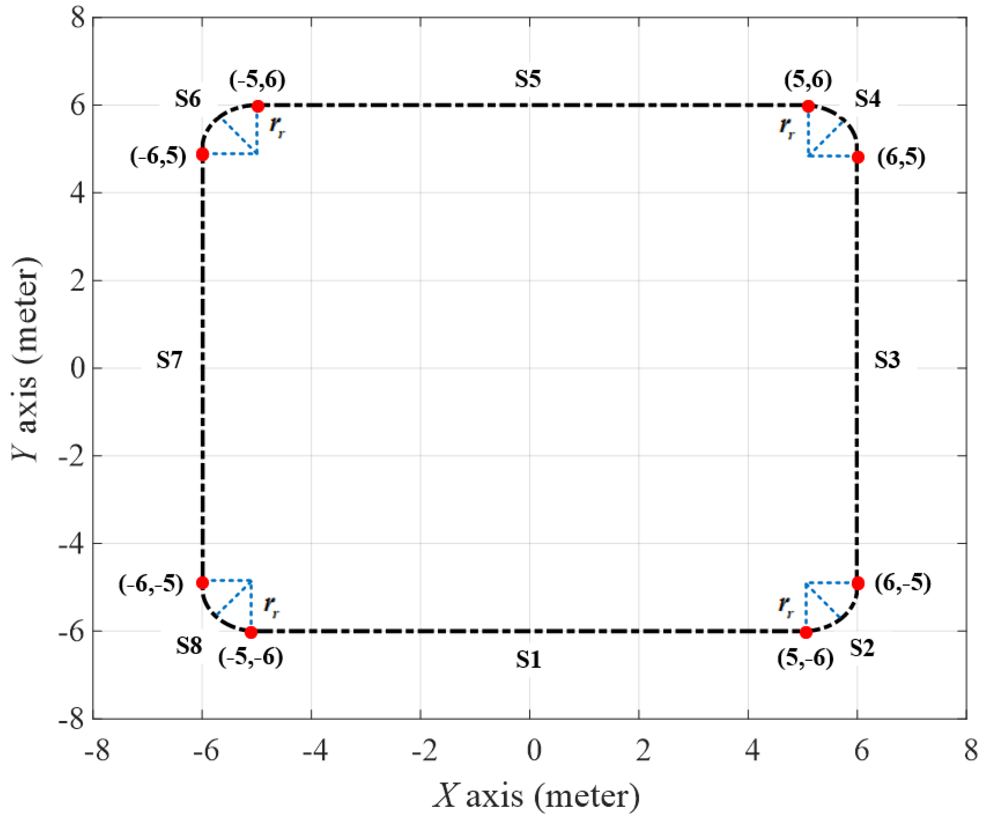
4.1. Setting of Simulation Environment

In this trajectory tracking verification, four AMRs corresponding to a practical AMR are used. The related system parameters of this practical AMR are given in

Table 1. System parameters of the controlled AMRs.

Description	Parameter	Value
AMR wheel radius	$r$	6.5 (cm)
AMR width	$2W$	35.6 (cm)
Distance from P to c	$d$	14 (cm)
AMR mass	$\overline{m}$	10 (kg)
AMR inertia	$I_P$	10 (kg-m2)

. The time-varying mass $m=\overline{m}+\Delta m$ is set up as the integration of a nominal value $\overline{m}$ = 10(Kg) and a disturbed value for Δm, which is a 20% variation of $\overline{m}$ for simulating the practical situation of AMRs carrying different goods. In addition, the desired square-type trajectory is constructed with eight segments: s1, s2, …, s8 of sub-trajectories; the brief descriptions for these sub-trajectories are introduced, as follows.

Equation (59) shows that s1 starts from the initial value $\left(x_0,y_0\right)$ and moves forward to the right-hand side, with a moving velocity of $v_r$.

$$s1:\{\begin{array}{l}{x}_{r1}=x_0+v_r{t}_1\\ y_{r1}=y_0\\ {\theta }_{r1}=0\end{array}$$

(59)

Using Equation (59), s1 starts from the initial value $\left(x_0,y_0\right)$ and moves forward to the right-hand side with a moving velocity of $v_r$.

The first curve s2 of this desired trajectory, which is one-quarter of a circular trajectory with a radius $r_r$, can be generated using the following equation:

$$s2:\{\begin{array}{l}{x}_{r2}=x_{r1}+r_r\cos ({\theta }_{r2}+{270}^{°})\\ y_{r2}=y_{r1}+r_r\sin ({\theta }_{r2}+{270}^{°})\\ {\theta }_{r2}={\displaystyle {\int }_{t_1}^{t_2}{\omega }_r}dt\end{array}$$

(60)

where $\left(x_{r1},y_{r1}\right)$ is the final value of the first segment s1, and ${\theta }_{r2}$ is the rotation angle of s2.

The erect segment s3 of this trajectory is expressed as follows:

$$s3:\{\begin{array}{l}{x}_{r3}=x_{r2}\\ y_{r3}=y_{r2}+v_r{t}_3\\ {\theta }_{r3}={90}^{°}\end{array}$$

(61)

where $\left(x_{r2},y_{r2}\right)$ is the final value of the first segment s2; ${\theta }_{r3}={90}^{°}$ shows that this segment, when is use, is perpendicular to s1.

Similarly, the second curve s4 of this trajectory can be presented as:

$$s4:\{\begin{array}{l}{x}_{r4}=x_{r3}+r_r\cos ({\theta }_{r4})\\ y_{r4}=y_{r3}+r_r\sin ({\theta }_{r4})\\ {\theta }_{r4}={\displaystyle {\int }_{t_3}^{t_4}{\omega }_r}dt+{90}^{°}\end{array}$$

(62)

where $\left(x_{r3},y_{r3}\right)$ is the final value of the first segment s1, and ${\theta }_{r4}$ is the rotation angle of s4.

The segment of the desired trajectory, which moves in the reverse direction of s1, with a velocity of $v_r$ and a constant ${\theta }_{r5}={90}^{°}$ is presented as:

$$s5:\{\begin{array}{l}{x}_{r5}=x_4-v_r{t}_5\\ y_{r5}=y_{r4}\\ {\theta }_{r5}={180}^{°}\end{array}$$

(63)

where $\left(x_{r4},y_{r4}\right)$ is the final value of the first segment, s5.

The third curve s6 of this trajectory can be presented as:

$$s6:\{\begin{array}{l}{x}_{r6}=x_{r5}+r_r\cos ({\theta }_{r6}+{90}^{°})\\ y_{r6}=y_{r5}+r_r\sin ({\theta }_{r6}+{90}^{°})\\ {\theta }_{r6}={\displaystyle {\int }_{t_5}^{t_6}{\omega }_r}dt+{180}^{°}\end{array}$$

(64)

where $\left(x_{r5},y_{r5}\right)$ is the final value of the first segment s5, and ${\theta }_{r6}$ is the rotation angle of s6.

The seven segments of this desired trajectory comprise an erect segment that is parallel to s3, as well as having a velocity $v_r$ and a constant ${\theta }_{r5}={270}^{°}$, and is expressed as:

$$s7:\{\begin{array}{l}{x}_{r7}=x_{r6}\\ y_{r7}=y_{r6}-v_r{t}_7\\ {\theta }_{r7}={270}^{°}\end{array}$$

(65)

where $\left(x_{r6},y_{r6}\right)$ is the final value of the first segment s5.

Finally, the fourth curve s8 of this desired trajectory can be expressed as:

$$s8:\{\begin{array}{l}{x}_{r8}=x_{r7}+r_r\cos ({\theta }_{r8}+{180}^{°})\\ y_{r8}=y_{r7}+r_r\sin ({\theta }_{r8}+{180}^{°})\\ {\theta }_{r8}={\displaystyle {\int }_{t_7}^{t_8}{\omega }_r}dt+{270}^{°}\end{array}$$

(66)

where $\left(x_{r7},y_{r7}\right)$ is the final value of the first segment s7, and ${\theta }_{r8}$ is the rotation angle of s6.

In this investigation, the desired square-type trajectory is generated using Equations (59)–(66) and is shown as in Figure 2; the initial conditions of this desired trajectory are set up as x₀ = −5(m), $y_0=-6(\mathrm{m})$, and ${\omega }_r=3^{°}/s$.

Remark 1.

The reason why we chose this desired trajectory as a testing scenario for our proposed method is as almost any trajectory, such as an s-shaped trajectory, trapezoidal-type trajectory, circle trajectory, or even wild trajectories, can be constructed using a combination of the above-mentioned segments and adjustments of the trajectory parameters, such as the velocity $v_r$, the rotation angle ${\theta }_{ri}$, and the radius $r_r$ for practical applications.

In this control trajectory tracking verification, four AMRs are chosen; the velocity $v_r$ and the radius $r_r$ are set up as 0.8 m/s for 1 m, respectively. As to the rotation angle ${\theta }_{ri}$, for i = 1, …, 4 can be calculated via integrating ${\omega }_r=3^{°}/s$, as depicted in the above equations. The control parameters of this proposed method are gained from Equations (67)–(69).

$${\rho }_T=diag\left(0.5,0.5,\dots ,0.5\right)$$

(67)

$$R=diag\left(0.3,0.3,\dots ,0.3\right)$$

(68)

$$\Xi =diag\left(I_{3\times 3},I_{3\times 3},\dots ,I_{3\times 3}\right)$$

(69)

The initial conditions of the controlled AMRs are given in

Table 2. Initial positions and attitudes of a swarm of AMRs.

Number of the Controlled AMR	$\mathbf{Initial}\mathbf{Position}({\mathit{x}}_{\mathit{p}},{\mathit{y}}_{\mathit{p}})$	Attitude $\mathit{\theta }$
#1 (Blue color)	(7,7)	$5\pi /4$
#2 (Green color)	(−7,7)	$7\pi /4$
#3 (Purple color)	(−7,−7)	$\pi /4$
#4 (Red color)	(7,−7)	$3\pi /4$

.

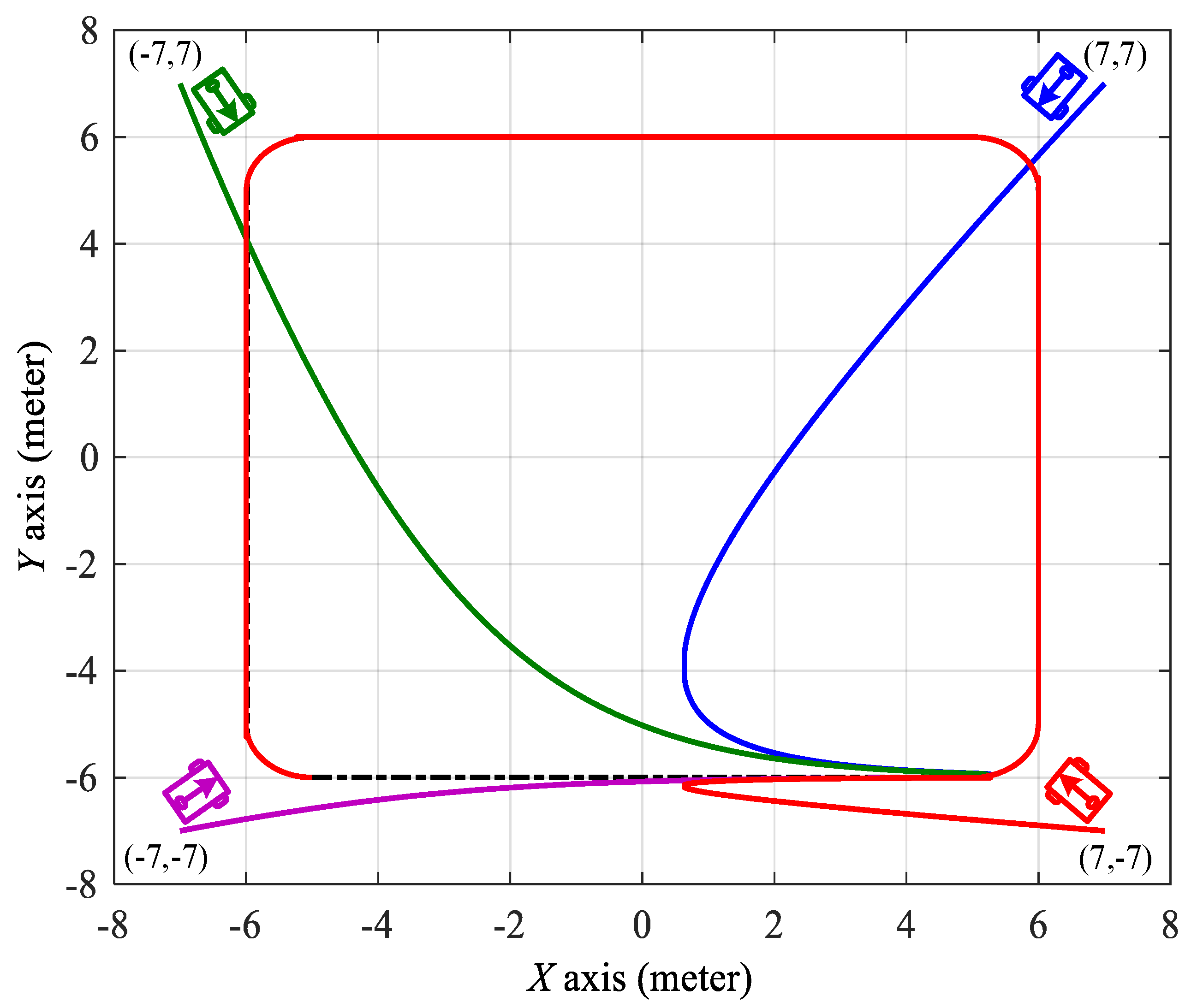
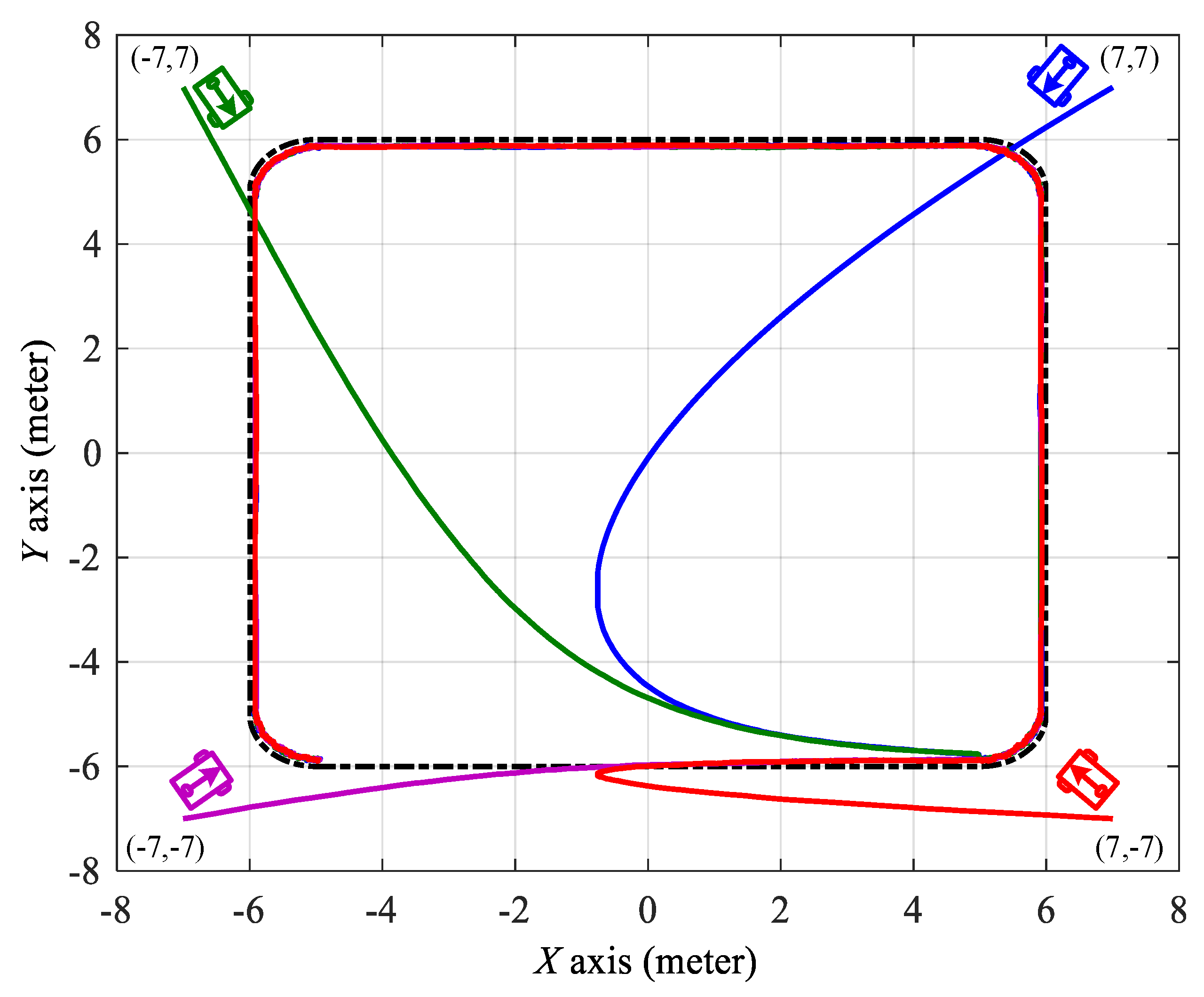
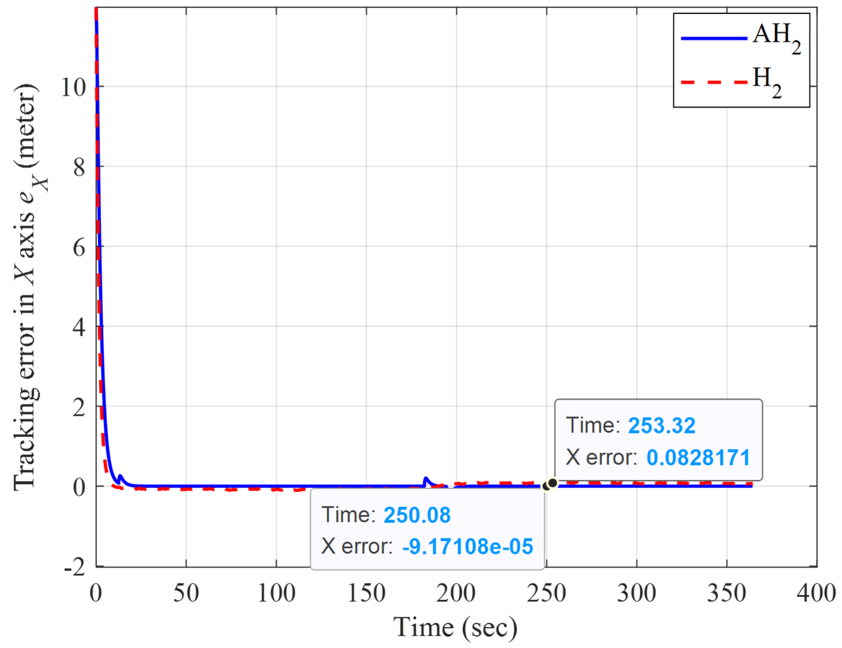
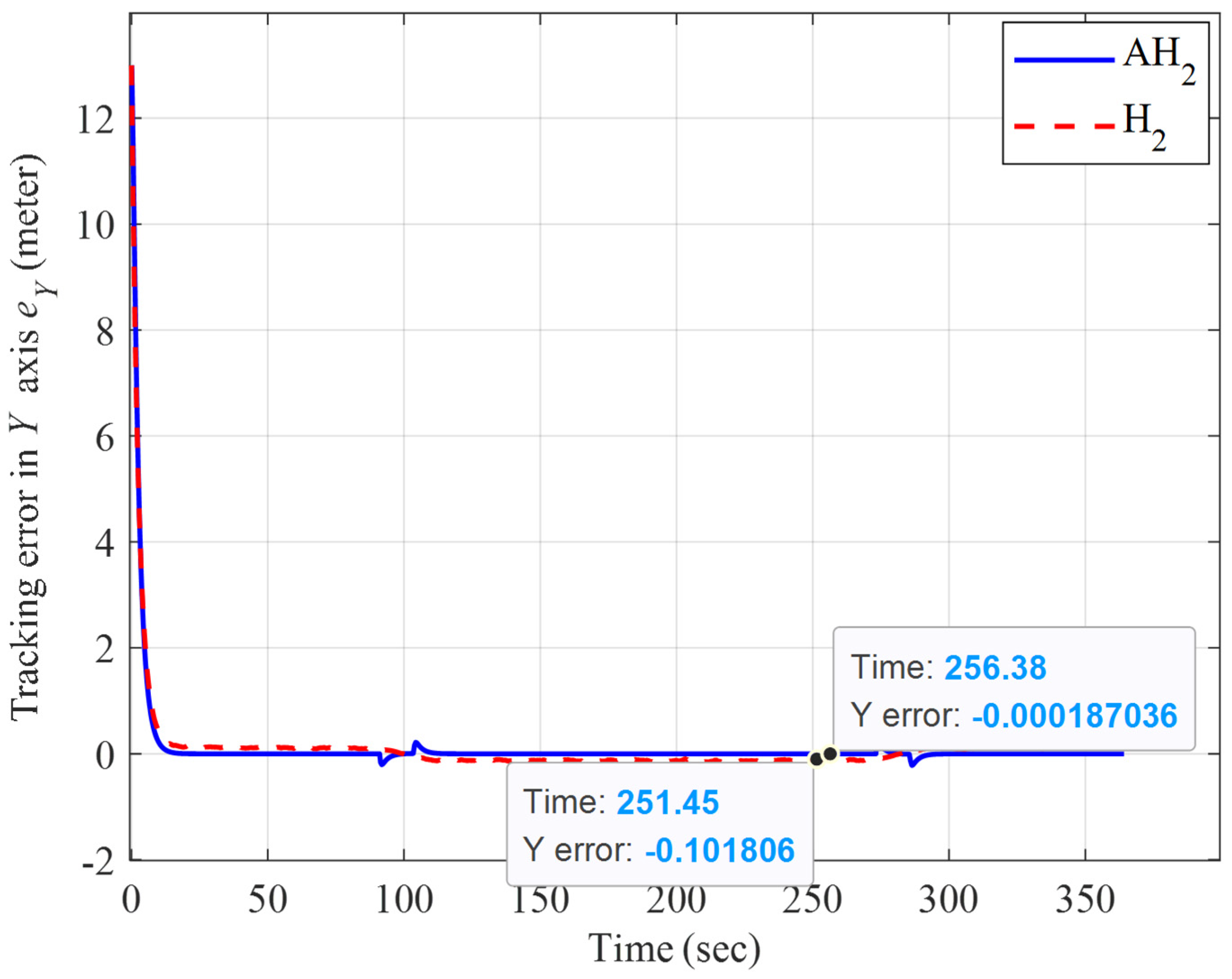
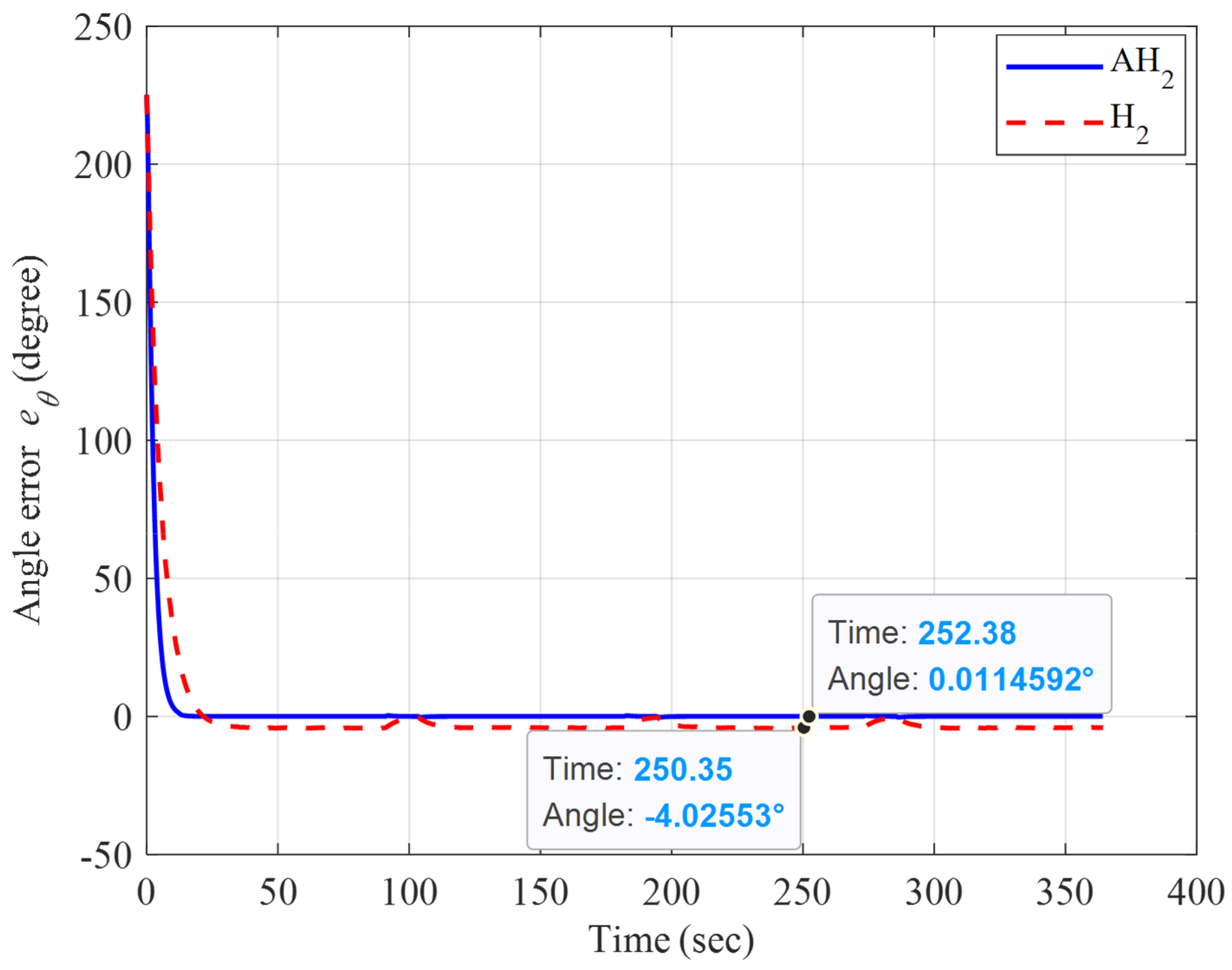
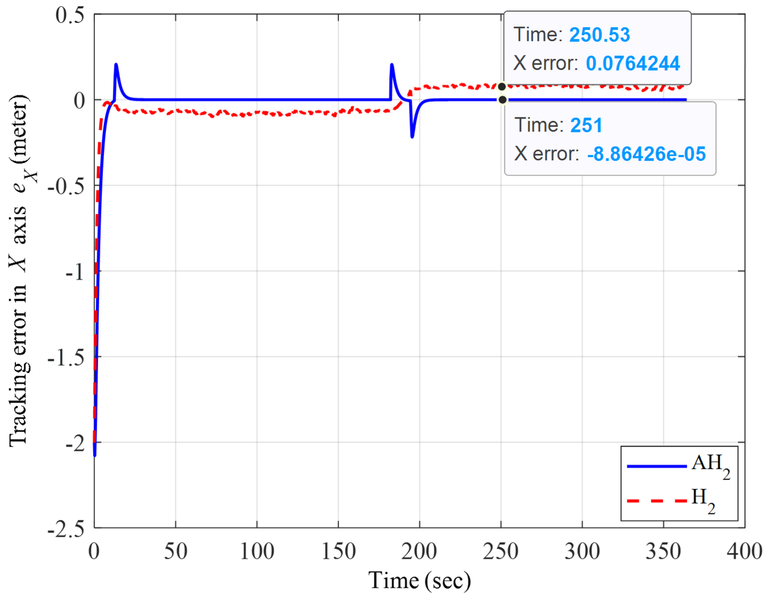
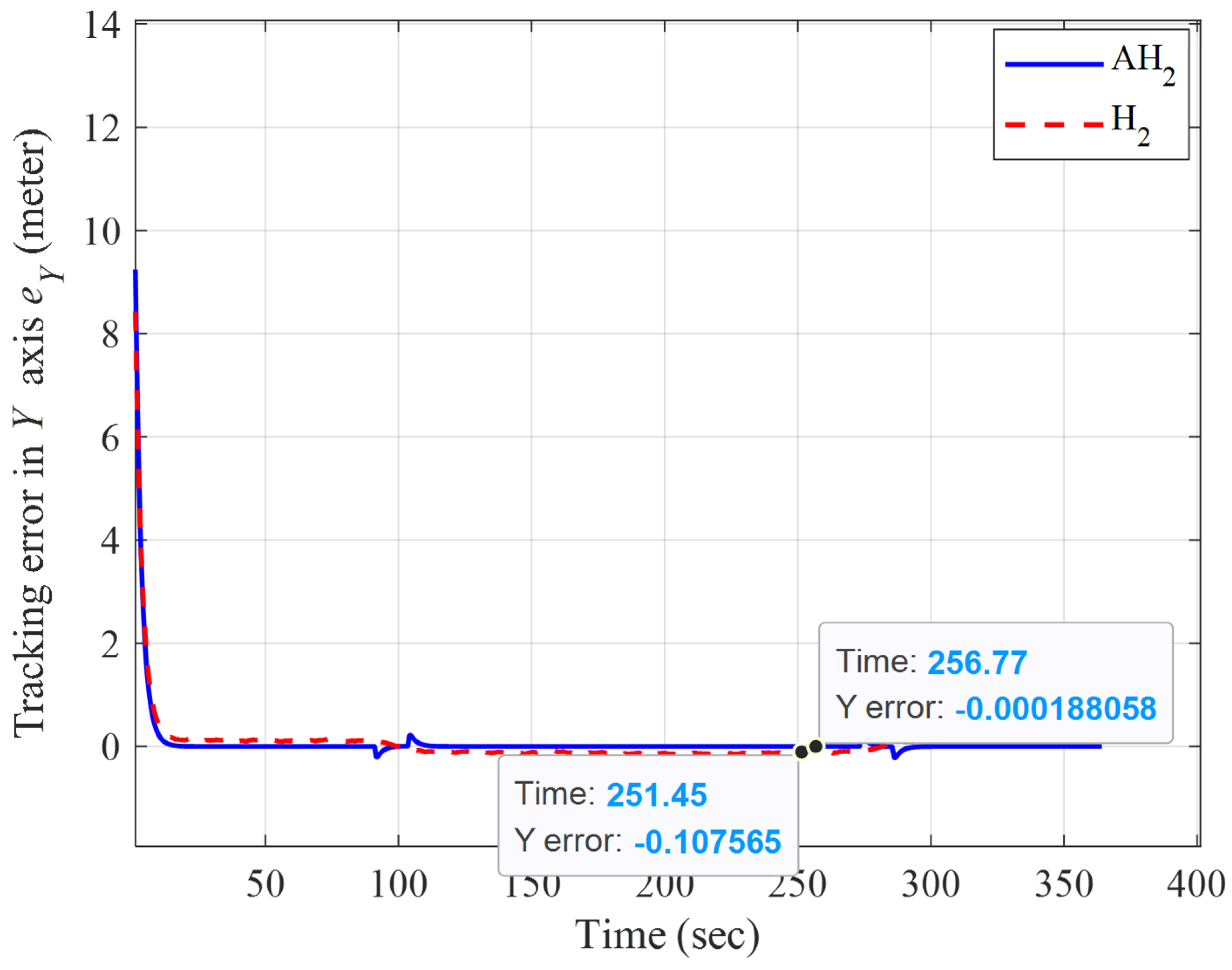
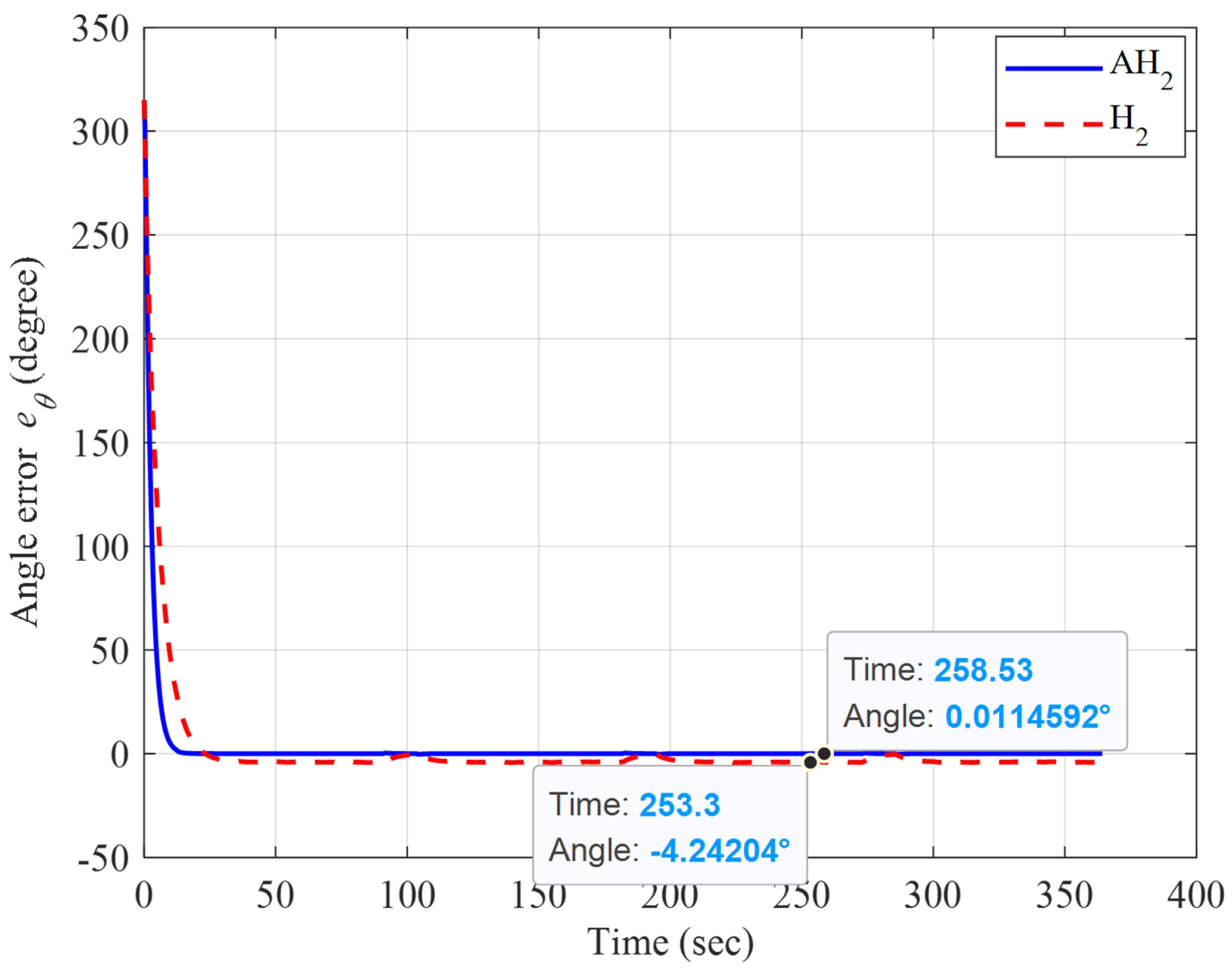
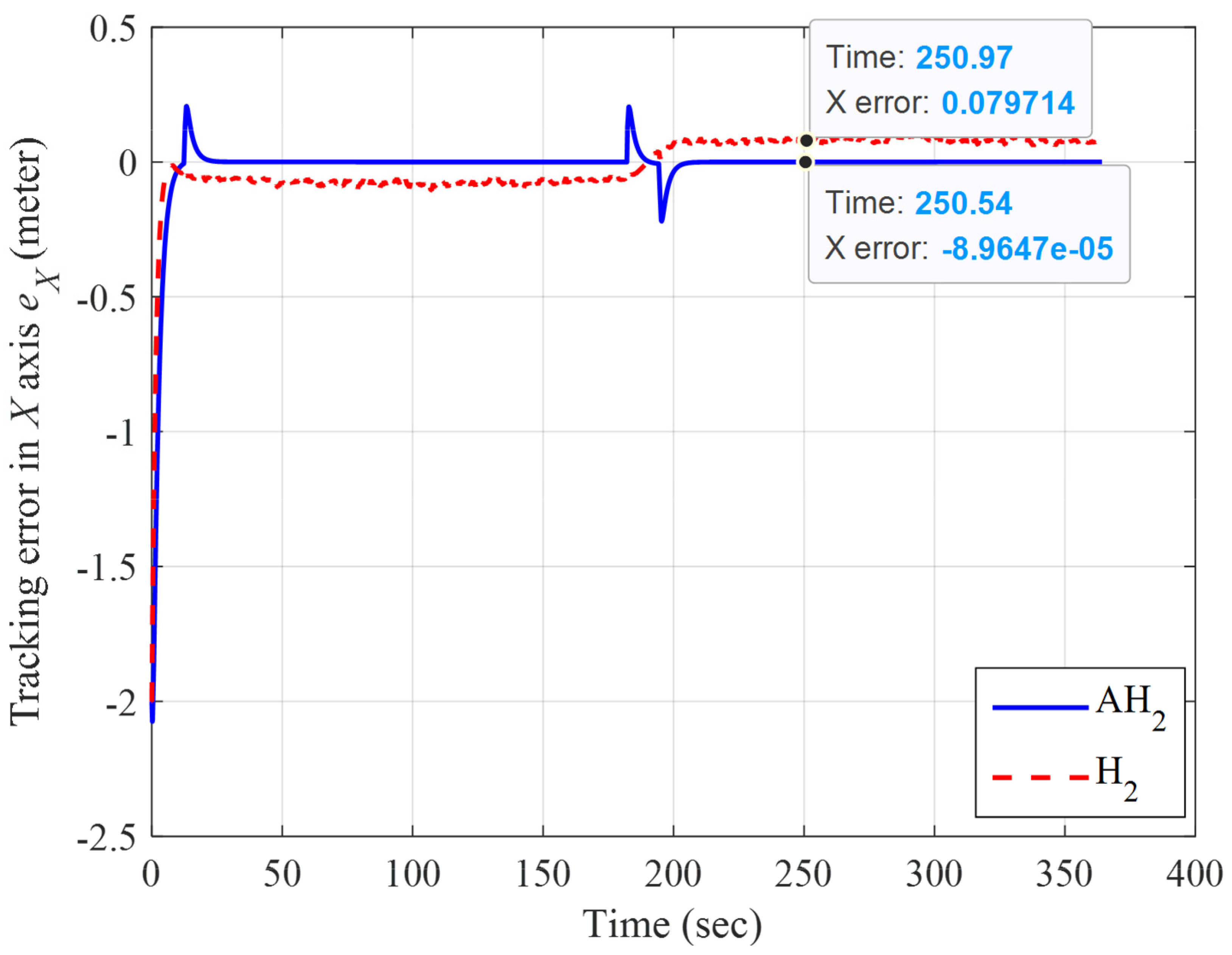
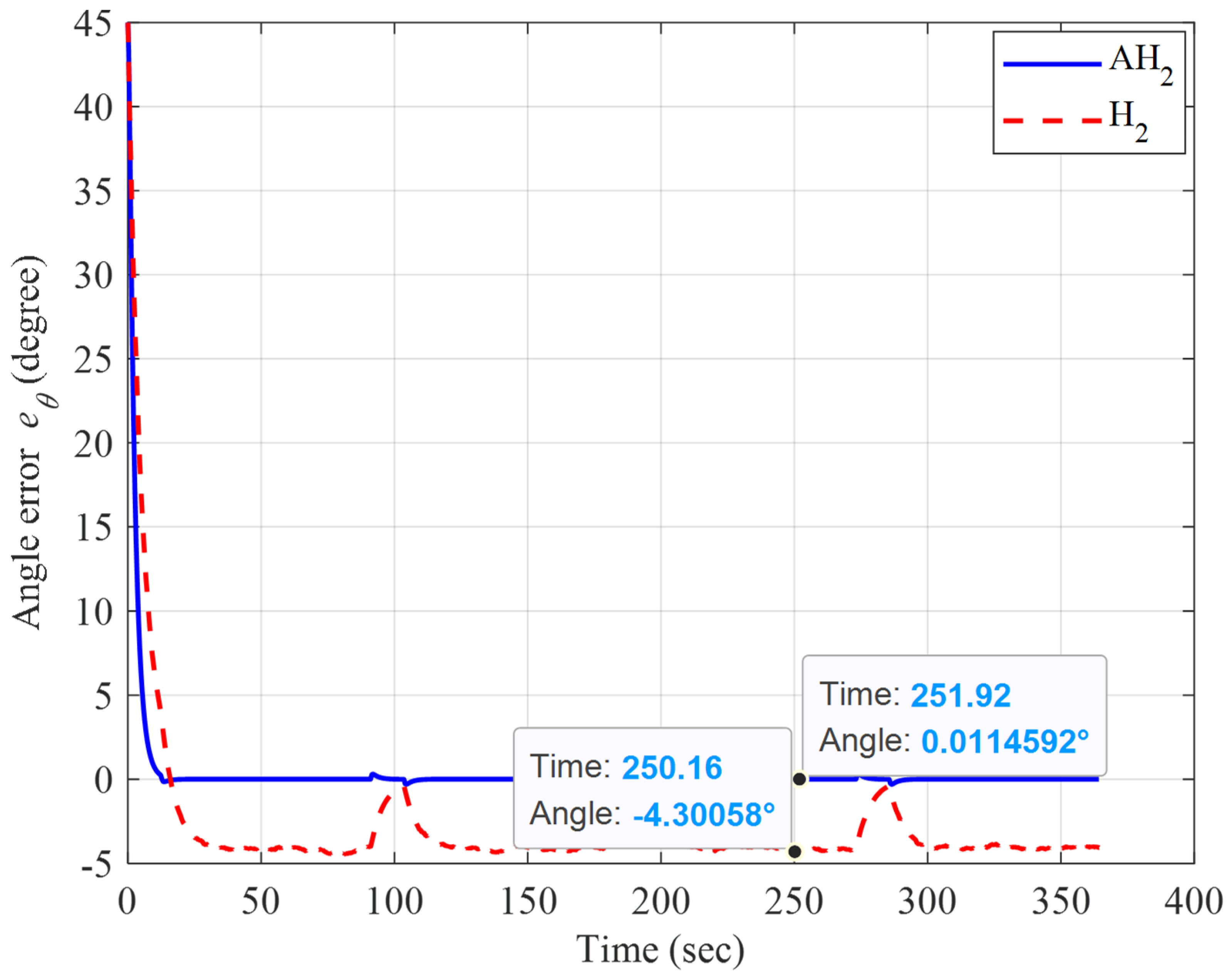
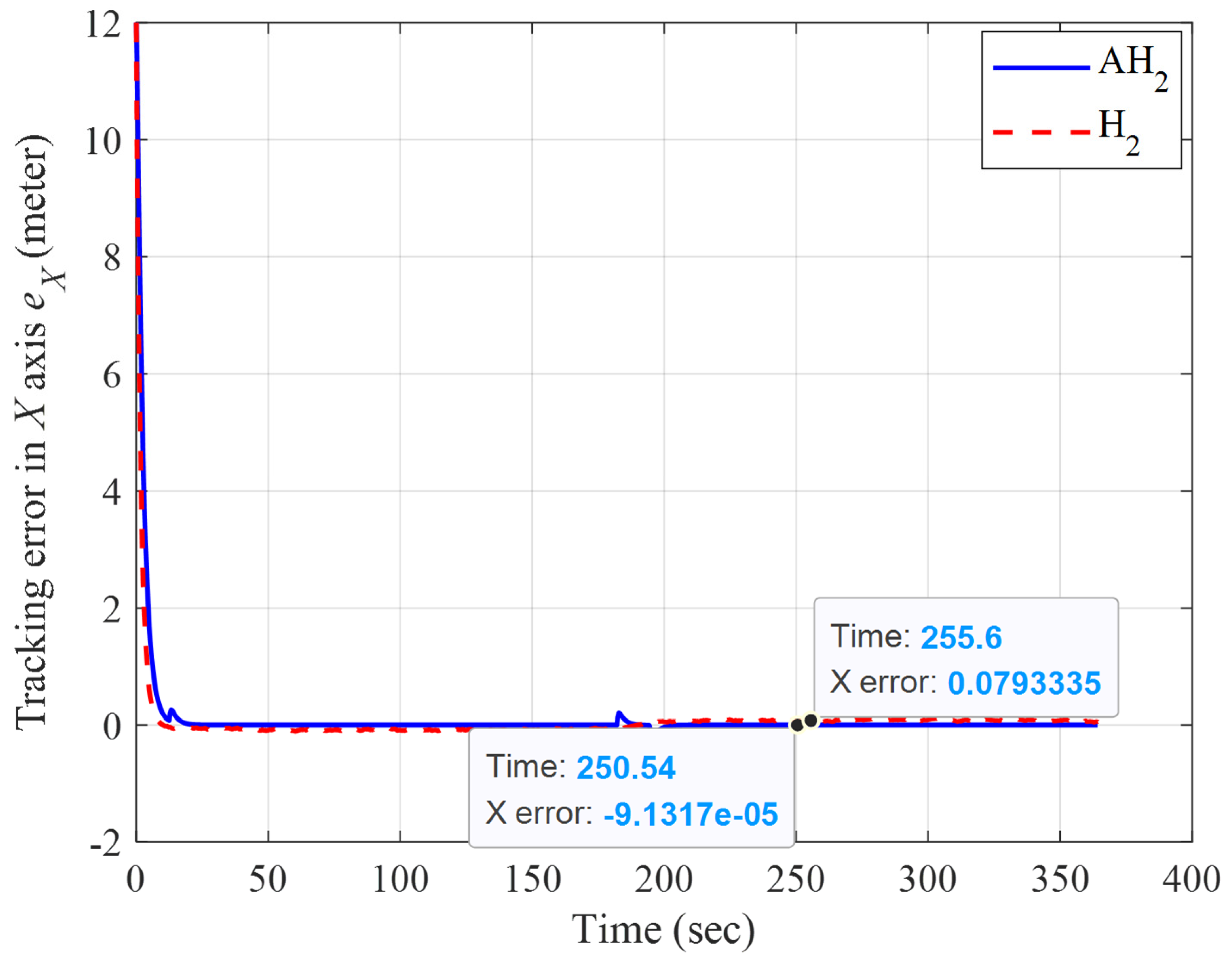
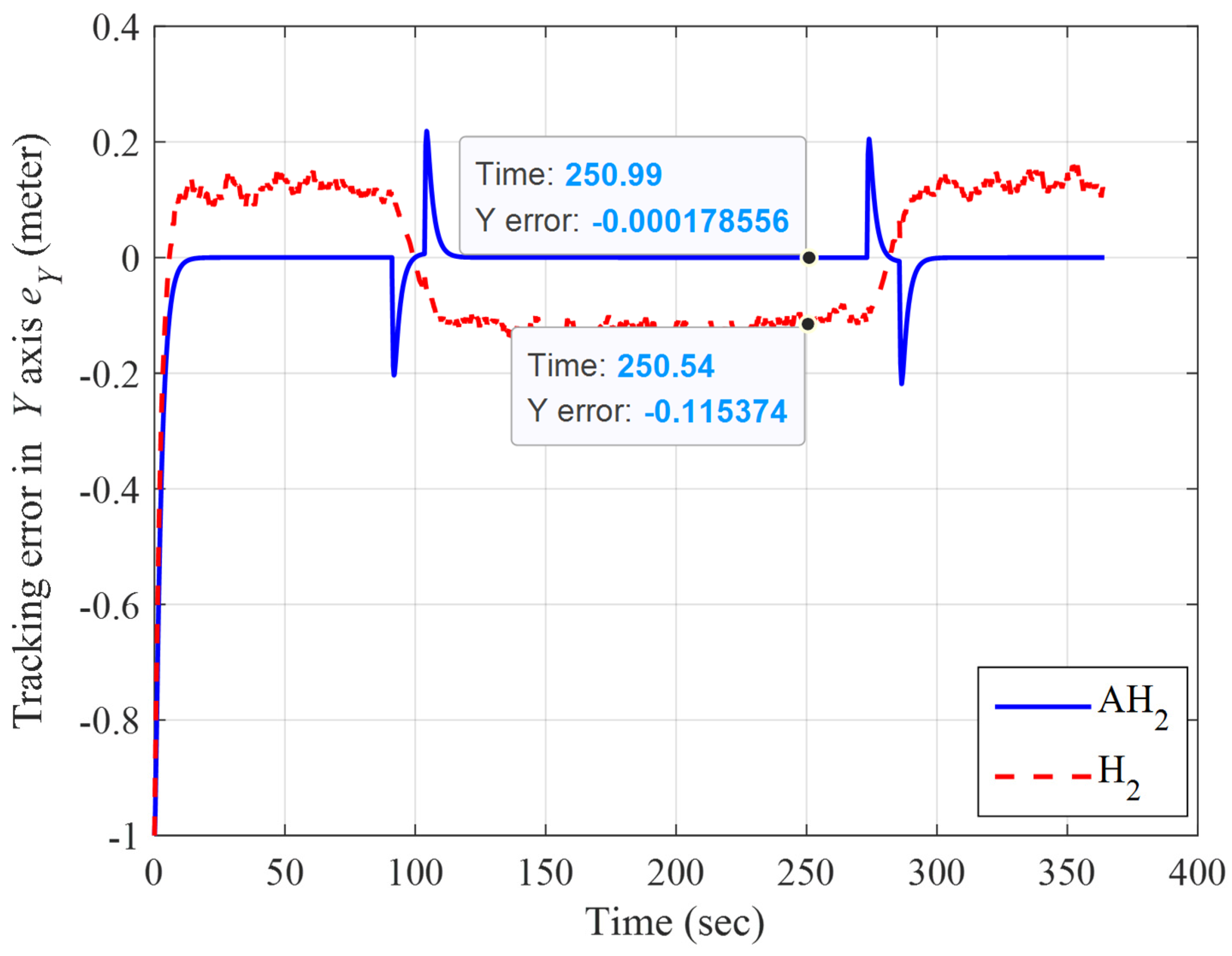
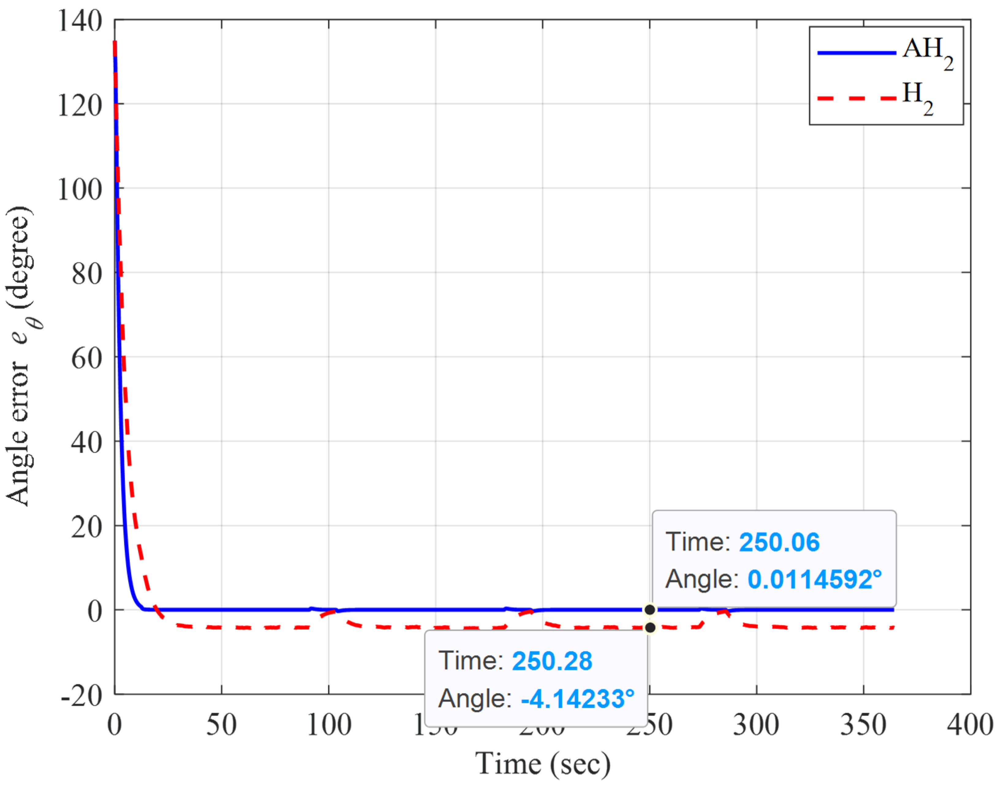
4.2. Simulation Results

For comparisons, a published H₂ closed-form control approach is adopted in this investigation [33]. Four AMRs with system parameters in Table 1, initial conditions listed in Table 2, and control gains from Equations (67)–(69) are considered in this trajectory tracking performance verification. For avoiding confusion, the trajectory tracking results of this proposed method (AH₂) and the H₂ closed-form control method (H₂) will be revealed separately in the following discussion. Figure 3 and Figure 4 show the trajectory tracking results of four AMRs controlled using the AH₂ and H₂ methods, with respect to the desired square-type trajectory. From Figure 3 and Figure 4, a similar tracking performance can be found for these two control methods. Obviously, the AMRs in Figure 3, controlled by the proposed AH₂ method, have quicker convergence rates in tracking the desired trajectory than with the H₂ method from the trajectory profiles.

Tracking errors, including errors ($e_{Xi}$, $e_{Yi}$, $e_{\theta i}$), for $i=1,\dots ,4$, in the X-axis, Y-axis, and the heading angle of the individual AMR are illustrated in the following figures. Figure 5, Figure 6 and Figure 7 depict the histories of tracking errors $e_X$, $e_Y$, and $e_{\theta }$ for the #1 AMR, using the AH₂ and H₂ method. From these tracking results, it is easy to establish that the trajectory tracking performance of the H₂ method is worse than the proposed AH₂ method because of the existence of steady state errors in $e_{X1}$, $e_{Y1}$, and $e_{\theta 1}$ under the effects of the 20% modeling uncertainties caused by Δm. The trajectory tracking errors $e_{X1}$, $e_{Y1}$, and $e_{\theta 1}$ of the #1 AMR, which converge to almost zero, can be transparently observed from Figure 5, Figure 6 and Figure 7. Similar tracking results can be found from Figure 8, Figure 9, Figure 10, Figure 11, Figure 12, Figure 13, Figure 14, Figure 15 and Figure 16 for #2 AMR, #3 AMR and #4 AMR. From these results, the proposed AH₂ method obviously outperforms the H₂ method.

According to the above trajectory tracking verification, this proposed AH₂ method ${\tau }^{\prime }(E(t),t)=\mathsf{\Phi }(t)\widehat{\xi }(t)+\frac{1}{\epsilon }{U}^{*}(E(t),t)$, which can precisely estimate the time-varying system parameters: ($m_i,d_i,I_i$) via adaptive learning law: $\dot{\widehat{\xi }}(t)=-R^{-1}{\mathsf{\Phi }}^T(t){\Xi }_T^{T}E(t)$, is superior to the H₂ method, which is constructed with fixed system parameters: (${\overline{m}}_i,{\overline{d}}_i,{\overline{I}}_i$).

5. Conclusions

A nonlinear adaptive optimal control design that presents good energy-saving performance has been successfully developed for the trajectory tracking problem of a swarm of autonomous mobile robots in this study. In the past few decades, complex control structures have always been revealed as part of the announced control laws because of the sub-optimal control approach. The most challenging part of this investigation has been to identify the closed-form solution for this trajectory tracking problem of a swarm of autonomous mobile robots. According to our survey of the existing published literature, the analytical solution for the trajectory tracking problem of a swarm of autonomous mobile robots has not been achieved yet, due to the great complexity of its dynamics. For achieving this design target, one main contribution is delivered in this investigation: “An analytical control solution, which has the simplest and easy-to-implemented control structure for the trajectory tracking problem of a swarm of autonomous mobile robots is elegantly derived”. In practice, complicated control structures mean that the cost in terms of computation consumption will be great and a high-speed calculator is always needed. From the comparisons of this proposed method with respect to a published H₂ method, which is an analytical solution as well, the control performance of this proposed method is superior to the H₂ method, no matter what the convergence of tracking errors or the elimination of modeling uncertainties.

References

1. Ibari, B.; Benchikh, L.; Elhachimi, A.R.; Ahmed-Foitih, Z. Backstepping Approach for Autonomous Mobile Robot Trajectory Tracking. J. Elect. Eng. Comp. Sci. 2016, 2, 478–485. [Google Scholar]
2. Mohammad, H.; Alireza, M. Trajectory Tracking Wheeled Mobile Robot Using Backstepping Method with Connection off Axle Trailer. Int. J. Smart Elect. Eng. 2018, 7, 177–187. [Google Scholar]
3. Wu, X.; Jin, P.; Zou, T.; Qi, Z.; Xiao, H.; Lou, P. Backstepping Trajectory Tracking Based on Fuzzy Sliding Mode Control for Differential Mobile Robots. J. Intell. Robot. Syst. 2019, 96, 109–121. [Google Scholar] [CrossRef]
4. Lu, E.; Ma, Z.; Li, Y.; Xu, L.; Tang, Z. Adaptive Backstepping Control of Tracked Robot Running Trajectory Based on Real-Time Slip Parameter Estimation. Int. J. Agric. Biol. Eng. 2020, 13, 178–187. [Google Scholar] [CrossRef]
5. Niraj, K.G.; Prabin, K.P. Sliding Mode Controller Design for Trajectory Tracking of a Non-Holonomic Mobile Robot with Disturbance. Comput. Electr. Eng. 2018, 72, 307–323. [Google Scholar]
6. Wang, G.; Zhou, C.; Yu, Y.; Liu, X. Adaptive Sliding Mode Trajectory Tracking Control for AMR Considering Skidding and Slipping via Extended State Observer. Energies 2019, 12, 3305. [Google Scholar] [CrossRef] [Green Version]
7. Aquib, M.; Narendra, K.D.; Nishchal, K.V. Event-Triggered Sliding Mode Control for Trajectory Tracking of Nonlinear Systems. IEEE/CAA J. Autom. Sin. 2020, 7, 307–314. [Google Scholar]
8. Li, J.; Wu, Q.; Wang, J.; Li, J. Neural Networks-Based Sliding Mode Tracking Control for the Four Wheel-Legged Robot Under Uncertain Interaction. Int. J. Robust Nonlinear Cont. 2021, 31, 4306–4323. [Google Scholar] [CrossRef]
9. Taniguchi, T.; Sugeno, M. Trajectory Tracking Controls for Non-Holonomic Systems Using Dynamic Feedback Linearization Based on Piecewise Multi-Linear Models. J. Appl. Math. 2017, 47, 339–351. [Google Scholar]
10. Chen, Y.Y.; Chen, Y.H.; Huang, C.Y. Autonomous Mobile Robot Design with Robustness Properties. Adv. Mech. Eng. 2018, 10, 1–11. [Google Scholar]
11. Mahmoodabadi, M.J.; Nejadkourki, N. Trajectory Tracking of a Flexible Robot Manipulator by a New Optimized Fuzzy Adaptive Sliding Mode-Based Feedback Linearization Controller. J. Robot. 2020, 2020, 8813217. [Google Scholar] [CrossRef]
12. Velagic, J.; Osmic, N.; Lacevic, B. Neural Network Controller for Mobile Robot Motion Control. Int. J. Intell. Syst. Tech. 2008, 47, 127–132. [Google Scholar]
13. Pavol, B.; Yury, L.K.; Andrey, A.A.; Kirill, S.Y. Neural Network Control of a Wheeled Mobile Robot Based on Optimal Trajectories. Int. J. Adv. Robot. Sys. 2020, 17, 1729881420916077. [Google Scholar]
14. Yu, J.; Su, Y.; Liao, Y. The Path Planning of Mobile Robot by Neural Networks and Hierarchical Reinforcement Learning. Fron. in Neur. 2020, 14, 1–12. [Google Scholar] [CrossRef] [PubMed]
15. Chen, Z.; Liu, Y.; He, W.; Qiao, H.; Ji, H. Adaptive-Neural-Network-Based Trajectory Tracking Control for a Nonholonomic Wheeled Mobile Robot with Velocity Constraints. IEEE Trans. Ind. Electron. 2021, 68, 5057–5067. [Google Scholar] [CrossRef]
16. Wu, T.F.; Xu, Q.; Kan, J.; Chen, S.; Yan, S. Fuzzy PID Based Trajectory Tracking Control of Mobile Robot and its Simulation in Simulink. Int. J. Control. Autom. 2014, 7, 233–244. [Google Scholar]
17. Chen, Y.H. A Novel Fuzzy Control Law for Nonholonomic Mobile Robots. Int. J. Comp. Intel. Cont. 2018, 5, 53–59. [Google Scholar]
18. Tiep, D.K.; Lee, K.; Im, D.Y.; Kwak, B.; Ryoo, Y.J. Design of Fuzzy-PID Controller for Path Tracking of Mobile Robot with Differential Drive. Int. J. Fuzzy Log. Intell. Syst. 2018, 18, 220–228. [Google Scholar] [CrossRef]
19. Hacene, N.; Mendil, B. Fuzzy Behavior-Based Control of Three Autonomous Omnidirectional Mobile Robot. Int. J. Autom. Comput. 2019, 16, 163–185. [Google Scholar] [CrossRef]
20. Abdelwahab, M.; Parque, V. Trajectory Tracking of Autonomous Mobile Robots Using Z-Number Based Fuzzy Logic. IEEE Access 2020, 8, 18426–18441. [Google Scholar] [CrossRef]
21. Huang, C.-J.; Chen, Y.-H.; Chao, C.-H.; Cheng, C.-F. A Fuzzy Control Design for the Trajectory Tracking of Autonomous Mobile Robot. Adv. Robot. Mech. Eng. 2020, 2, 206–211. [Google Scholar] [CrossRef]
22. Du, Q.; Sha, L.; Shi, W.; Sun, L. Adaptive Fuzzy Path Tracking Control for Mobile Robots with Unknown Control Direction. Discret. Dyn. Nat. Soc. 2021, 2021, 9935271. [Google Scholar] [CrossRef]
23. Dixon, W.E.; Dawson, D.M.; Zergeroglu, E.; Behal, A. Adaptive Tracking Control of a Wheeled Mobile Robot via an Uncalibrated Camera System. IEEE Trans. Syst. Man Cybern. Part B 2001, 31, 341–352. [Google Scholar] [CrossRef] [PubMed] [Green Version]
24. Chen, P.; Mitsutake, S.; Isoda, T.; Shi, T. Omni-Directional Robot and Adaptive Control Method for Off-Road Running. IEEE Trans. Robot. Autom. 2002, 18, 251–256. [Google Scholar] [CrossRef]
25. Mohamed, S.; Yamada, A.; Sano, S.; Uchiyama, N. Design of a Redundant Autonomous Drive System for Energy Saving and Fail Safe Motion. Adv. Mech. Eng. 2016, 8, 1687814016676074. [Google Scholar] [CrossRef] [Green Version]
26. Rigatos, G.; Busawon, K.; Pomares, J.; Abbaszadeh, M. Nonlinear Optimal Control for a Spherical Rolling Robot. Int. J. Intell. Robot. Appl. 2019, 3, 221–237. [Google Scholar] [CrossRef]
27. Hu, Y.; Su, H.; Zhang, L.; Miao, S.; Chen, G.; Knoll, A. Nonlinear Model Predictive Control for Mobile Robot Using Varying-Parameter Convergent Differential Neural Network. Robotics 2019, 8, 64. [Google Scholar] [CrossRef] [Green Version]
28. Rigatos, G.; Busawon, K.; Pomares, J.; Abbaszadeh, M. Nonlinear Optimal Control for the Wheeled Inverted Pendulum System. Robotica 2020, 38, 29–47. [Google Scholar] [CrossRef]
29. Askhat, D.; Elena, S.; Ivan, Z. Optimal Control Problem Solution with Phase Constraints for Group of Robots by Pontryagin Maximum Principle and Evolutionary Algorithm. Mathematics 2020, 8, 2105. [Google Scholar]
30. Mishra, S.K.; Jha, A.V.; Verma, V.K.; Appasani, B.; Abdelaziz, A.Y.; Bizon, N. An Optimized Triggering Algorithm for Event-Triggered Control of Networked Control Systems. Mathematics 2021, 9, 1262. [Google Scholar] [CrossRef]
31. Chen, Y.H.; Li, T.H.S.; Chen, Y.Y. A Novel Nonlinear Control Law with Trajectory Tracking Capability for Mobile Robots: Closed-Form Solution Design. Appl. Math. Inf. Sci. 2013, 7, 749–754. [Google Scholar] [CrossRef]
32. Chen, Y.H.; Lou, S.J. Control Design of a Swarm of Intelligent Robots: A Closed-Form H2 Nonlinear Control Approach. Appl. Sci. 2020, 10, 1055. [Google Scholar] [CrossRef] [Green Version]
33. Chen, Y.H.; Chen, Y.Y.; Lou, S.J.; Huang, C.J. Energy Saving Control Approach for Trajectory Tracking of Autonomous Mobile Robots. Intell. Autom. Soft Comput. 2021, 30, 357–372. [Google Scholar] [CrossRef]
Figure 1. Schematics of the controlled AMR.
Mathematics 10 03901 g001
Figure 2. The desired square trajectory, with a radius of 6 m from x0 = −5 m, y0 = −6 m.
Mathematics 10 03901 g002
Figure 3. The verification result of the square trajectory by the adaptive H2 closed-form control approach from xp = 7 m, yp = 7 m (blue line), xp = −7 m, yp = 7 m (green line), xp = −7 m, yp = −7 m (purple line), xp = 7 m, yp = −7 m (red line).
Mathematics 10 03901 g003
Figure 4. The verification result of the square trajectory by the H2 closed-form control approach from xp = 7 m, yp = 7 m (blue line), xp = −7 m, yp = 7 m (green line), xp = −7 m, yp = −7 m (purple line), xp = 7 m, yp = −7 m (red line).
Mathematics 10 03901 g004
Figure 5. The square trajectory tracking result of the adaptive H2 closed-form and H2 closed-form control approaches for the x-axis from xp = 7 m, yp = 7 m.
Mathematics 10 03901 g005
Figure 6. The square trajectory tracking result of the adaptive H2 closed-form and H2 closed-form control approaches for the y-axis from xp = 7 m, yp = 7 m.
Mathematics 10 03901 g006
Figure 7. The square trajectory tracking result of the adaptive H2 closed-form and H2 closed-form control approaches for an angle from xp = 7 m, yp = 7 m.
Mathematics 10 03901 g007
Figure 8. The square trajectory tracking error result of the adaptive H2 closed-form and H2 closed-form control approaches for the x-axis from xp = −7 m, yp = 7 m.
Mathematics 10 03901 g008
Figure 9. The square trajectory tracking error result of the adaptive H2 closed-form and H2 closed- form control approaches for the y-axis from xp = −7 m, yp = 7 m.
Mathematics 10 03901 g009
Figure 10. The square trajectory tracking error result of the adaptive H2 closed-form and H2 closed-form control approaches for an angle from xp = −7 m, yp = 7 m.
Mathematics 10 03901 g010
Figure 11. The square trajectory tracking error result of the adaptive H2 closed-form and H2 closed-form control approaches for an x-axis from xp = −7 m, yp = −7 m.
Mathematics 10 03901 g011
Figure 12. The square trajectory tracking error result of the adaptive H2 closed-form and H2 closed-form control approach for the y-axis from xp = −7 m, yp = −7 m.
Mathematics 10 03901 g012
Figure 13. The square trajectory tracking error result of the adaptive H2 closed-form and H2 closed-form control approaches for angle from xp = −7 m, yp = −7 m.
Mathematics 10 03901 g013
Figure 14. The square trajectory tracking error result of the adaptive H2 closed-form and H2 closed-form control approaches for X from xp = 7 m, yp = −7 m.
Mathematics 10 03901 g014
Figure 15. The square trajectory tracking error result of the adaptive H2 closed-form and H2 closed-form control approaches for Y from xp = 7 m, yp = −7 m.
Mathematics 10 03901 g015
Figure 16. The square trajectory tracking error result of the adaptive H2 closed-form and H2 closed-form control approaches for an angle from xp = 7 m, yp = −7 m.
Mathematics 10 03901 g016