The Calculation of the Probability Density and Distribution Function of a Strictly Stable Law in the Vicinity of Zero

Abstract

The problem of calculating the probability density and distribution function of a strictly stable law is considered at $x\to 0$. The expansions of these values into power series were obtained to solve this problem. It was shown that in the case $\alpha <1$, the obtained series were asymptotic at $x\to 0$; in the case $\alpha >1$, they were convergent; and in the case $\alpha =1$ in the domain $\left|x\right|<1$, these series converged to an asymmetric Cauchy distribution. It has been shown that at $x\to 0$ the obtained expansions can be successfully used to calculate the probability density and distribution function of strictly stable laws.

1. Introduction

The major inconvenience of using stable laws is the absence of expressions for the probability density and distribution function in terms of elementary functions. There are only five cases known where the density is expressed in terms of elementary functions: the L$\acute{e}$vy distribution ($\alpha =1/2,\theta =1$), the symmetric L$\acute{e}$vy distribution ($\alpha =1/2,\theta =-1$), the Cauchy distribution ($\alpha =1,\theta =0$), the Gaussian distribution ($\alpha =2,\theta =0$), and the asymmetric Cauchy distribution ($\alpha =1,-1⩽\theta ⩽1$) (see Formulas (5) and (8)). Here $\alpha$ is a characteristic exponent of the stable law that $\theta$ is a parameter of asymmetry. The latter distribution was first described in a book by V.M. Zolotarev [1] (see formula (2.3.5a)) and was later examined in works [2,3]. Different representations for stable laws are required to calculate the probability density or distribution function in other cases.

Paper [4] shows that if values of the characteristic exponent $\alpha$ and the asymmetry parameter $\beta$ are limited by values of rational numbers ($\alpha =P/Q$, $\beta =U/V$, where $P,Q,V$ are positive integers), then in this case, it is possible to express the probability density of a strictly stable law in terms of special functions. Papers [4,5,6,7,8,9,10] are devoted to obtaining such representations. The limitation of this approach lies in the fact that it is possible to obtain an expression for the probability density only for rational values of the parameters $\alpha$ and $\beta$ and only for strictly stable laws. The application of the fast Fourier transform algorithm is another method of calculating density. This approach has been examined in papers [11,12]. However, this method provides an opportunity for the calculation of the probability density on a grid of equidistant points. In this paper, linear interpolation must be used to calculate the density at intermediate points or irregularly spaced points.

The use of integral representations is the main method for calculating the probability density and the distribution function of stable laws. This approach is based on the inversion Formula (2). There are two possible ways of inverting the characteristic function. The first way is to directly calculate the integral in (2). As a result, the probability density is expressed in terms of the integral of the oscillating function [13,14]. However, since the integrand is an oscillating function, this leads to difficulties in numerical integration in the cases $\alpha <0.75$, $\beta \ne 0$, and $0<|\alpha -1|<0.001$ and in the case of large values x [13]. Modernization of the standard quadrature method of numerical integration makes it possible to reduce the lower boundary of the parameter $\alpha$ from the value $0.75$ to the value $0.5$ [14]. It has been proposed to use the representation of the density in the form of a power series to calculate the density for large values of x.

The second way of obtaining integral representations is the application of the stationary phase method when calculating the integral in (2) (see [1,3,15,16]). The advantage of this method of inverting the characteristic function is that the resulting integral representation is expressed in terms of a definite integral of a monotonic function. Such integral representations were obtained for stable laws with different parameterizations of the characteristic function. These were obtained for the parameterization “B” in works [1,15], for the parameterization of “M” in paper [16], and for the parameterization of “C” in paper [3]. Here the notation of various parameterizations of the characteristic function is given in accordance with the designations introduced in the book by V.M. Zolotarev [1]. These integral representations are more convenient from a practical point of view and allow calculating the density in a wide range of parameter values $\alpha ,\beta$, and coordinates x. The integral representation obtained in the work [16] served as a foundation for developing several software products [17,18,19,20,21].

From a theoretical point of view, these integral representations are valid for all values of x. However, in practice, it is not possible to calculate the probability density and distribution function for all values of x. The reason for this lies in the behavior of the integrand. The integrand has the form of a very sharp peak with small and large values of x. As a result, numerical integration algorithms cannot correctly calculate the integral in this range of x. To settle this issue, in papers [16,18,19] the use of various numerical methods to increase the accuracy of calculations was proposed. However, all proposed approaches increase the accuracy of the calculation but do not completely eliminate the problem. To calculate the probability density and distribution function in this range of values of x, it is expedient to use other representations for stable laws which do not have any specific features in the indicated areas. The approach used in papers [12,14] seems to be the most suitable, which consists of applying expansions in a power series for probability density and distribution function with $x\to 0$ and $x\to \infty$.

Such expansions are well known and are obtained, as a rule, for the parametrization “B”. Depending on the value of the parameter $\alpha$, the obtained power series is either convergent or asymptotic. The expansion of the probability density of a stable law into a convergent series in the case $x\to \infty$ and $0<\alpha <1$ was firstly mentioned in paper [22]. Later, in paper [23] a generalization of this density expansion was given for $x\to \infty$ in the case $1<\alpha <2$. In this range of values of the parameter $\alpha$, this series turns out to be asymptotic. In the same paper, the expansion of the density in a series in the vicinity of the point $x\to 0$ was obtained for the case $0<\alpha <2$. The resulting power series is asymptotic in the case $0<\alpha <1$ and convergent in the case $1<\alpha <2$. Expansions for $\alpha >1$ in the cases of $x\to 0$ and $x\to \infty$ were also obtained in the work [5] as a result of expansion into a power series of the probability density, expressed in terms of the Fox function. The same expansions were given in the books [24] (see Chapter 17, §7) and [1] (see §2.4 and §2.5). Expansions of the density of a stable law in a power series for the characteristic function in parameterization “M” were obtained in paper [14]. An interesting result was obtained in paper [25]. In this paper, expansions of the power series were obtained for the probability density of a symmetric stable law at $x\to 0$ and $x\to \infty$ for the cases $0<\alpha <1$ and $1<\alpha <2$. A distinctive property of this expansion is that these power series for all $\alpha$ are convergent.

The purpose of this work is to obtain power series expansions of the probability density and distribution function of a strictly stable law with the characteristic function

$$\widehat{g}(t,\alpha ,\theta ,\lambda )=\exp \left\{-{\lambda \left|t\right|}^{\alpha }\exp \{-i\frac{\pi }{2}\alpha \theta \mathrm{sign}t\}\right\},t\in \mathbf{R},$$

(1)

where $\alpha \in (0,2]$, $\left|\theta \right|⩽\min (1,2/\alpha -1)$, $\lambda >0$. This parameterization of the characteristic function, according to the book [1], is called parameterization “C”. Obtaining such expansions turns out to be necessary in connection to the problem of calculating the probability density and distribution function of stable and fractionally stable laws. In fact, in the article [3], integral representations were obtained for the probability density and distribution function of a strictly stable law with the characteristic function (1). Because these integral representations were obtained using the stationary phase method, the integrand has the form of a very sharp peak when the value of the coordinate x is either large or small. This causes difficulties for numerical integration algorithms and leads to incorrect integration results. Therefore, to calculate the probability density and distribution function in these coordinate regions, it is expedient to use representations in the form of a power series for the corresponding quantities. This work is devoted to obtaining such expansions.

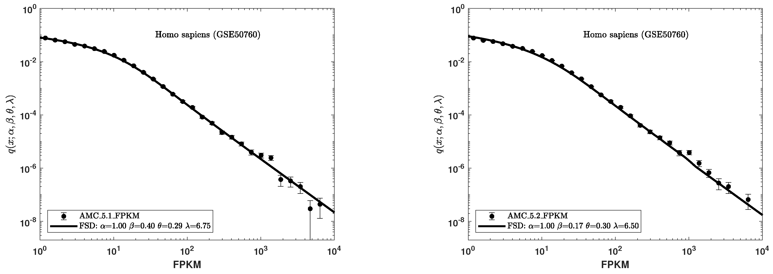
The solution to this problem will turn out to be useful not only when calculating the density of strictly stable laws but also in the task of calculation the density and distribution function of a fractional-stable law [2,26,27] (for more details see Appendix A). These distributions are expressed in terms of the Mellin convolution of two strictly stable laws. Correct calculation of the probability density will make it possible to use an algorithm for statistical estimation of the parameters of these laws based on the maximum likelihood method. Such an algorithm for estimating parameters will provide an opportunity to correctly describe various experimental data. It is known that the distribution of gene expression is described by laws with a power-law decrease in density [28,29,30]. Since the stable and fractionally stable densities decrease according to the power law $x^{-\alpha -1}$ at $x\to \infty$, then these classes of distributions were used to describe the distribution of gene expression (Appendix A). In the works [31,32], fractional stable distributions were used to describe the expression of genes obtained using microarray technology. In the work [33], these distributions were used to describe the results obtained using next generation sequencing technology. To describe these experimental data, it is necessary to have algorithms for the statistical estimation of parameters, the most effective of which is the maximum likelihood method. To construct such an algorithm, it is necessary to be able to correctly calculate the density of a strictly stable law for any values of x.

2. Preliminary Remarks

The major purpose of this work is to obtain the expansions of the density and distribution function of a strictly stable law in a power series in the vicinity of the point $x=0$. This paper deals with strictly stable laws with the characteristic function (1). Without loss of generality, we will assume that the scale parameter $\lambda =1$. Strictly stable laws with the parameter $\lambda =1$ are commonly called standard strictly stable laws. Designation abbreviations are accepted for standard strictly stable laws. The characteristic function will be designated by $\widehat{g}(t,\alpha ,\theta ,1)\equiv \widehat{g}(t,\alpha ,\theta )$, the probability density distribution will be designated by $g(x,\alpha ,\theta ,1)\equiv g(x,\alpha ,\theta )$, and the distribution function will be designated by $G(x,\alpha ,\theta ,1)\equiv G(x,\alpha ,\theta )$.

To perform the inverse Fourier transform and obtain the probability density distribution, the following lemma is useful, which defines the inversion formula

Lemma 1.

The probability density function $g(x,\alpha ,\theta )$ for any admissible set of parameters $(\alpha ,\theta )$ and any x can be obtained using the inversion formulas

$$g(x,\alpha ,\theta )=\frac{1}{2\pi }{\int }_{-\infty }^{\infty }{e}^{-itx}\widehat{g}(t,\alpha ,\theta )dt=\left\{\begin{array}{c}{\displaystyle \frac{1}{\pi }\Re {\int }_0^{\infty }{e}^{itx}\widehat{g}(t,\alpha ,-\theta )dt,}\\ {\displaystyle \frac{1}{\pi }\Re {\int }_0^{\infty }{e}^{-itx}\widehat{g}(t,\alpha ,\theta )dt.}\end{array}\right.$$

(2)

The proof of this lemma can be found in paper [3]. To obtain the probability density, there is no fundamental difference based on which formula is used on the right side (2). The result will differ only in the sign of the parameter $\theta$. Without loss of generality, in this paper we will use the first Formula (2). Such a choice results from the fact that in works [1,3,34], this formula was used to invert the characteristic function. This will provide us with an opportunity to compare the results obtained below with the results of the mentioned papers without any additional transformations.

In article [3], the inverse Fourier transform of the characteristic function (1) was performed and expressions for the probability density and distribution function of a strictly stable law were obtained. In the case $\alpha \ne 1$ and $x\ne 0$ for any admissible $\theta$, the following integral representation is true for the probability density

$$g(x,\alpha ,\theta )=\frac{\alpha }{\pi |\alpha -1|}{\int }_{-\pi {\theta }^{*}/2}^{\pi /2}\exp \left\{-{\left|x\right|}^{\alpha /(\alpha -1)}U(\phi ,\alpha ,{\theta }^{*})\right\}U(\phi ,\alpha ,{\theta }^{*}){\left|x\right|}^{1/(\alpha -1)}d\phi ,$$

(3)

where ${\theta }^{*}=\theta \mathrm{sign}\left(x\right)$ and

$$U(\phi ,\alpha ,\theta )={\left(\frac{\sin \left(\alpha \left(\phi +\frac{\pi }{2}\theta \right)\right)}{\cos \phi }\right)}^{\frac{\alpha }{1-\alpha }}\frac{\cos \left(\phi (1-\alpha )-\frac{\pi }{2}\alpha \theta \right)}{\cos \phi }.$$

(4)

If $\alpha =1$, then for any admissible $-1⩽\theta ⩽1$ the probability density has the form

$$g(x,1,\theta )=\frac{\cos (\pi \theta /2)}{\pi \left(x^2-2x\sin (\pi \theta /2)+1\right)}.$$

(5)

If $x=0$, then $g(0,\alpha ,\theta )=\frac{1}{\pi }\cos (\pi \theta /2)\mathsf{\Gamma }(1/\alpha +1)$.

The following expressions are valid for the distribution function. If $\alpha \ne 1$, then for any admissible $\theta$

$$G(x,\alpha ,\theta )=\frac{1}{2}(1-\mathrm{sign}\left(x\right))+\mathrm{sign}\left(x\right)G^{(+)}\left(\right|x|,\alpha ,{\theta }^{*}),$$

(6)

where

$$\begin{array}{c}{G}^{(+)}(x,\alpha ,\theta )=1-\frac{1+\theta }{4}(1+\mathrm{sign}(1-\alpha ))\hfill \\ \hfill +\frac{\mathrm{sign}(1-\alpha )}{\pi }{\int }_{-\pi \theta /2}^{\pi /2}\exp \left\{-x^{\alpha /(\alpha -1)}U(\phi ,\alpha ,\theta )\right\}d\phi ,\end{array}$$

(7)

$x>0$ and $U(\phi ,\alpha ,\theta )$ is determined by expression (4). If $\alpha =1$, then for any $-1⩽\theta ⩽1$

$$G(x,1,\theta )=\frac{1}{2}+\frac{1}{\pi }\arctan \left(\frac{x-\sin \left(\frac{\pi }{2}\theta \right)}{\cos \left(\frac{\pi }{2}\theta \right)}\right).$$

(8)

In the point $x=0$, for any admissible $\alpha$ and $\theta$

$$G(0,\alpha ,\theta )=\frac{1}{2}(1-\theta ).$$

(9)

To obtain the density representation $g(x,\alpha ,\theta )$ in the form of power series, the integral obtained in the book [35] (see §1.5. formula (31)) turns out to be useful.

$${\int }_0^{\infty }{t}^{\gamma -1}{e}^{-ct\cos \beta -ict\sin \beta }dt=\mathsf{\Gamma }\left(\gamma \right)c^{-\gamma }{e}^{-i\gamma \beta }$$

under the conditions $-\frac{\pi }{2}<\beta <\frac{\pi }{2},\Re \gamma >0\mathrm{or}\beta =\pm \frac{\pi }{2},0<\Re \gamma <1$. If we use Euler’s formula $\cos \beta +i\sin \beta =e^{i\beta }$, then this integral can be represented in the form

$${\int }_0^{\infty }{t}^{\gamma -1}{e}^{-ct\exp \left\{i\beta \right\}}dt=\mathsf{\Gamma }\left(\gamma \right)c^{-\gamma }{e}^{-i\gamma \beta }$$

(10)

under the conditions $-\frac{\pi }{2}<\beta <\frac{\pi }{2},\Re \gamma >0$ or $\beta =\pm \frac{\pi }{2},0<\Re \gamma <1$.

3. Representation of the Probability Density in the Form of a Power Series

We obtain the expansion of the probability density $g(x,\alpha ,\theta )$ in a series at $x\to 0$. The following theorem is valid:

Theorem 1.

In the case $x\to 0$ for any admissible set of parameters $(\alpha ,\theta )$ except for the values $\alpha =1,\theta =\pm 1$ for the probability density $g(x,\alpha ,\theta )$, the following representation in the form of a series is valid

$$g(x,\alpha ,\theta )=g_N^0(x,\alpha ,\theta )+R_N^0,$$

(11)

where

$$\begin{array}{cc}\hfill g_N^0(x,\alpha ,\theta )& =\frac{1}{\alpha \pi }\sum _{n=0}^{N-1}\frac{x^n}{n!}\mathsf{\Gamma }\left(\frac{n+1}{\alpha }\right)\sin \left(\frac{\pi }{2}(n+1)(1-\theta )\right),\hfill \end{array}$$

(12)

$$\begin{array}{cc}\hfill |R_N^0|& ⩽\frac{1}{\alpha \pi }\frac{{\left|x\right|}^N}{N!}\mathsf{\Gamma }\left(\frac{N+1}{\alpha }\right)\hfill \end{array}$$

(13)

Proof. 

We will perform the inverse Fourier transform of the characteristic function (1). To perform this, we make use of the first relation in (2). We have

$$g(x,\alpha ,\theta )=\frac{1}{\pi }\Re {\int }_0^{\infty }{e}^{itx}\widehat{g}(t,\alpha ,-\theta )dt=\frac{1}{\pi }\Re {\int }_0^{\infty }\exp \left\{itx-t^{\alpha }\exp \left\{i\frac{\pi }{2}\alpha \theta \right\}\right\}dt.$$

Because the considered case is $x\to 0$, we expand $\exp \left\{itx\right\}$ in a series in the vicinity of the point $x=0$. As a result, we obtain:

$$g(x,\alpha ,\theta )=g_N^0(x,\alpha ,\theta )+R_N^0(x,\alpha ,\theta ),$$

(14)

where the N-th partial sum $g_N^0(x,\alpha ,\theta )$ and the remainder $R_N^0(x,\alpha ,\theta )$ of a series have the form

$$\begin{array}{cc}\hfill g_N^0(x,\alpha ,\theta )& =\frac{1}{\pi }\Re {\int }_0^{\infty }\exp \left\{-t^{\alpha }\exp \left\{i\frac{\pi }{2}\alpha \theta \right\}\right\}\sum _{n=0}^{N-1}\frac{{\left(itx\right)}^n}{n!}dt,\hfill \end{array}$$

(15)

$$\begin{array}{cc}\hfill R_N^0(x,\alpha ,\theta )& =\frac{1}{\pi }\Re {\int }_0^{\infty }\exp \left\{-t^{\alpha }\exp \left\{i\frac{\pi }{2}\alpha \theta \right\}\right\}{R}_N\left(itx\right)dt.\hfill \end{array}$$

(16)

Here $R_N\left(itx\right)=\frac{{\left(itx\right)}^N}{N!}{e}^{itx\zeta },(0<\zeta <1)$ is the remainder in the Lagrange form.

We then consider the N-th partial sum $g_N^0(x,\alpha ,\theta )$. To calculate the integral in (15), we change the order of summation and integration in some places and we will substitute the integration variable $t^{\alpha }=\tau$. As a result, we obtain

$$g_N^0(x,\alpha ,\theta )=\frac{1}{\alpha \pi }\sum _{n=0}^{N-1}\frac{x^n}{n!}\Re i^n{\int }_0^{\infty }{\tau }^{\frac{n+1}{\alpha }-1}\exp \left\{-\tau \exp \left\{i\frac{\pi }{2}\alpha \theta \right\}\right\}d\tau .$$

(17)

Next, we examine the range of valid values of the argument $\frac{\pi }{2}\alpha \theta$. The range of admissible values of the parameter $\theta$ is determined by the inequality $\left|\theta \right|⩽\min (1,2/\alpha -1)$. Hence, if $0<\alpha ⩽1$, then $-1⩽\theta ⩽1$, and if $1<\alpha ⩽2$, then $-(2/\alpha -1)⩽\theta ⩽2/\alpha -1$. Thus,

$$\frac{\pi }{2}\alpha \theta \in \left[\frac{\pi }{2}\alpha ,\frac{\pi }{2}\alpha \right]\in \left[-\frac{\pi }{2},\frac{\pi }{2}\right],\mathrm{if}0<\alpha ⩽1.$$

(18)

$$\frac{\pi }{2}\alpha \theta \in \left[\frac{\pi }{2}\alpha -\pi ,\pi -\frac{\pi }{2}\alpha \right]\in \left(-\frac{\pi }{2},\frac{\pi }{2}\right),\mathrm{if}1<\alpha ⩽2.$$

(19)

Combining (18) and (19), we obtain

$$-\frac{\pi }{2}⩽\frac{\pi }{2}\alpha \theta ⩽\frac{\pi }{2},\mathrm{if}0<\alpha ⩽2.$$

(20)

As we can see, extreme values of this range are reached in the cases $\alpha =1$ and $\theta =\pm 1$.

Taking into consideration (20), it is clear that on can use Formula (10) to calculate the integral in (17). We obtain

$${\int }_0^{\infty }{\tau }^{\frac{n+1}{\alpha }-1}\exp \left\{-\tau \exp \left\{i\frac{\pi }{2}\alpha \theta \right\}\right\}d\tau =\mathsf{\Gamma }\left(\frac{n+1}{\alpha }\right)\exp \left\{-i\frac{\pi }{2}(n+1)\theta \right\}.$$

(21)

From the relation (10) it follows that for the arbitrary value $(n+1)/\alpha >0$ it is necessary to exclude the case $\frac{\pi }{2}\alpha \theta =\pm \frac{\pi }{2}$ from consideration, which is implemented at values $\alpha =1,\theta =\pm 1$. Now using expression (21) in (17), we obtain

$$g_N^0(x,\alpha ,\theta )=\frac{1}{\alpha \pi }\sum _{n=0}^{N-1}\frac{x^n}{n!}\mathsf{\Gamma }\left(\frac{n+1}{\alpha }\right)\Re i^n\exp \left\{-i\frac{\pi }{2}(n+1)\theta \right\}.$$

Considering that now $\Re i^n\exp \left\{-i\frac{\pi }{2}(n+1)\theta \right\}=\sin \left(\frac{\pi }{2}(n+1)(1-\theta )\right)$, we finally obtain

$$g_N^0(x,\alpha ,\theta )=\frac{1}{\alpha \pi }\sum _{n=0}^{N-1}\frac{x^n}{n!}\mathsf{\Gamma }\left(\frac{n+1}{\alpha }\right)\sin \left(\frac{\pi }{2}(n+1)(1-\theta )\right).$$

Now we consider the remainder $R_N^0(x,\alpha ,\theta )$. From expression (16), we obtain

$$R_N^0=\frac{x^N}{\pi N!}\Re i^N{\int }_0^{\infty }\exp \left\{itx\zeta -t^{\alpha }\exp \left\{i\frac{\pi }{2}\alpha \theta \right\}\right\}{t}^{N}dt.$$

It is not possible to calculate this integral, as the exact value of the quantity $\zeta$ is not known. It is only known that $0<\zeta <1$. However, one can obtain an estimate for this integral. We have

$$\begin{array}{c}{R}_N^0(x,\alpha )⩽\left|R_N^0(x,\alpha )\right|⩽\frac{1}{\pi }\frac{{\left|x\right|}^N}{N!}\left|\Re i^N{\int }_0^{\infty }{t}^N\exp \left\{-t^{\alpha }\exp \left\{i\frac{\pi }{2}\alpha \theta \right\}\right\}{e}^{itx\zeta }dt\right|⩽\hfill \\ \frac{{\left|x\right|}^N}{\pi N!}\left(\left|\Re i^N{\int }_0^{\infty }{t}^N\exp \left\{-t^{\alpha }\exp \left\{i\frac{\pi }{2}\alpha \theta \right\}\right\}dt\right|\right)=\\ \frac{{\left|x\right|}^N}{\alpha \pi N!}\left(\left|\Re i^N{\int }_0^{\infty }{\tau }^{\frac{N+1}{\alpha }-1}\exp \left\{-\tau \exp \left\{i\frac{\pi }{2}\alpha \theta \right\}\right\}d\tau \right|\right)=\\ \hfill \frac{{\left|x\right|}^N}{\alpha \pi N!}\mathsf{\Gamma }\left(\frac{N+1}{\alpha }\right)\left|\Re i^N\exp \left\{-i\frac{\pi }{2}(N+1)\theta \right\}\right|⩽\frac{1}{\alpha \pi }\frac{{\left|x\right|}^N}{N!}\mathsf{\Gamma }\left(\frac{N+1}{\alpha }\right)\end{array}$$

To obtain the third inequality, it was taken into consideration that $\left|\exp \right\{itx\zeta \left\}\right|⩽1$. Next, the integration variable was substituted $t^{\alpha }=\tau$. To calculate the resulting integral, Formula (10) was used. The obtained expression completely proves the theorem. □

We need to make one small remark. When proving the theorem, it was pointed out that it was necessary to exclude the case $\frac{\pi }{2}\alpha \theta =\pm \frac{\pi }{2}$ from consideration, which corresponds to the values of parameters $\alpha =1,\theta \pm 1$. As part of the proof of the theorem, this was done so that the range of admissible values of the argument $\frac{\pi }{2}\alpha \theta$ of the integral in (17) should coincide with the range of admissible values of the argument $\beta$ included in the integral (10). However, the exception of the case $\beta =\pm \frac{\pi }{2}$ from the integral (10) is related to the fact that in these points the integral (10) will diverge (for details see [36]). Therefore, it should be assumed that $\alpha =1$ and $\theta =\pm 1$, and the integral in (17) will diverge. This in its turn leads to a degenerate probability density at that point. As a result, we arrive at the well-known fact that the probability density with the characteristic function (1) is degenerate at the points $\alpha =1,\theta \pm 1$.

As noted in the introduction, depending on the value of the parameter $\alpha$, the expansion of the probability density of the stable law in a power series turns out to be either convergent or divergent. Exactly the same situation occurs in the case considered here. The determine under what values of $\alpha$ the expansion (11) is convergent and for which it is divergent we formulate as a corollary

Corollary 1.

In the case $\alpha <1$, the series (12) is divergent at $N\to \infty$. In this case, for the density $g(x,\alpha ,\theta )$, for any admissible θ, the asymptotic expansion

$$g(x,\alpha ,\theta )\sim \frac{1}{\alpha \pi }\sum _{n=0}^{N-1}\frac{x^n}{n!}\mathsf{\Gamma }\left(\frac{n+1}{\alpha }\right)\sin \left(\frac{\pi }{2}(n+1)(1-\theta )\right),x\to 0.$$

is valid.

In the case $\alpha =1$, the series (12) converges for any x, satisfying the condition $\left|x\right|<1$. In the case of the density $g(x,1,\theta )$, for any admissible $\theta \ne \pm 1$ it is possible to represent in the form of an infinite series

$$g(x,1,\theta )=\frac{1}{\pi }\sum _{n=0}^{\infty }\sin \left(\frac{\pi }{2}(n+1)(1-\theta )\right)x^n,\left|x\right|<1.$$

(22)

In the case $\alpha >1$, the series (12) converges for any x. In this case, for the density $g(x,\alpha ,\theta )$ for any admissible θ it possible to represent in the form of an infinite series

$$g(x,\alpha ,\theta )=\frac{1}{\alpha \pi }\sum _{n=0}^{\infty }\frac{x^n}{n!}\mathsf{\Gamma }\left(\frac{n+1}{\alpha }\right)\sin \left(\frac{\pi }{2}(n+1)(1-\theta )\right).$$

Proof. 

We examine the convergence of the series (12). As we can see, this series is a sign-alternating series. Consequently,

$$\begin{array}{c}{g}_N^0(x,\alpha ,\theta )⩽\left|g_N^0(x,\alpha ,\theta )\right|⩽\frac{1}{\alpha \pi }\sum _{n=0}^{N-1}\frac{{\left|x\right|}^n}{n!}\mathsf{\Gamma }\left(\frac{n+1}{\alpha }\right)\left|\sin \left(\frac{\pi }{2}(n+1)(1-\theta )\right)\right|\hfill \\ \hfill ⩽\frac{1}{\alpha \pi }\sum _{n=0}^{N-1}\frac{{\left|x\right|}^n}{n!}\mathsf{\Gamma }\left(\frac{n+1}{\alpha }\right)\end{array}$$

We apply the Cauchy criterion in the limiting form to the resulting series.

$$\begin{array}{c}\underset{n\to \infty }{\lim }{\left(\frac{{\left|x\right|}^n}{\alpha \pi }\frac{\mathsf{\Gamma }\left((n+1)/\alpha \right)}{n!}\right)}^{1/n}=\underset{n\to \infty }{\lim }\frac{\left|x\right|}{{\left(\alpha \pi \right)}^{1/n}}{\left(\frac{\mathsf{\Gamma }\left((n+1)/\alpha \right)}{\mathsf{\Gamma }(n+1)}\right)}^{1/n}=\hfill \\ \left|x\right|\underset{n\to \infty }{\lim }{\left(\frac{\exp \left\{-\frac{n+1}{\alpha }\right\}{\left(\frac{n+1}{\alpha }\right)}^{\frac{n+1}{\alpha }-\frac{1}{2}}\sqrt{2\pi }}{\exp \left\{-n-1\right\}{(n+1)}^{n+1-\frac{1}{2}}\sqrt{2\pi }}\right)}^{\frac{1}{n}}=\\ \left|x\right|\underset{n\to \infty }{\lim }{e}^{\left(1+\frac{1}{n}\right)\left(1-\frac{1}{\alpha }\right)}{\alpha }^{-\frac{1}{\alpha }-\frac{1}{n}\left(\frac{1}{\alpha }-\frac{1}{2}\right)}{(n+1)}^{\left(1+\frac{1}{n}\right)\left(\frac{1}{\alpha }-1\right)}\\ \hfill =\left|x\right|e^{1-\frac{1}{\alpha }}{\alpha }^{-\frac{1}{\alpha }}\underset{n\to \infty }{\lim }{(n+1)}^{\left(\frac{1}{\alpha }-1\right)}=\left\{\begin{array}{cc}\infty ,& \alpha <1,\\ \left|x\right|,& \alpha =1,\\ 0,& \alpha >1.\end{array}\right.\end{array}$$

Here Stirling’s formula was used

$$\mathsf{\Gamma }\left(z\right)\sim e^{-z}{z}^{z-\frac{1}{2}}\sqrt{2\pi },z\to \infty ,\left|\arg z\right|<\pi .$$

(23)

From the result obtained we can see that for the values $\alpha <1$ the series (12) diverges for any x; with the value $\alpha =1$, the series (12) converges for any values of x, satisfying the condition $\left|x\right|<1$; and in the case $\alpha >1$, the series (12) converges for any x.

We consider the case $\alpha <1$. In this case, the series (12) diverges at $N\to \infty$. However, from expression (13) it follows that for some fixed N

$$R_N^0=O\left(x^N\right),x\to 0.$$

Thus, with every N we have

$$g(x,\alpha ,\theta )=\frac{1}{\alpha \pi }\sum _{n=0}^{N-1}\frac{x^n}{n!}\mathsf{\Gamma }\left(\frac{n+1}{\alpha }\right)\sin \left(\frac{\pi }{2}(n+1)(1-\theta )\right)+O\left(x^N\right),x\to 0.$$

As a result, we have obtained the definition of an asymptotic series. Consequently,

$$g(x,\alpha ,\theta )\sim \frac{1}{\alpha \pi }\sum _{n=0}^{N-1}\frac{x^n}{n!}\mathsf{\Gamma }\left(\frac{n+1}{\alpha }\right)\sin \left(\frac{\pi }{2}(n+1)(1-\theta )\right),x\to 0,\alpha <1.$$

We consider the case $\alpha >1$. From expression (11) it follows that

$$|g(x,\alpha ,\theta )-g_N^0(x,\alpha ,\theta )|⩽\frac{1}{\alpha \pi }\frac{\mathsf{\Gamma }\left(\frac{N+1}{\alpha }\right)}{N!}{\left|x\right|}^N.$$

(24)

We will set some arbitrary x and consider the limit of the right-hand side of this inequality under the condition $N\to \infty$. We have

$$\begin{array}{c}\frac{1}{\alpha \pi }\underset{N\to \infty }{\lim }\frac{\mathsf{\Gamma }\left(\frac{N+1}{\alpha }\right)}{N!}{\left|x\right|}^N=\frac{1}{\alpha \pi }\underset{N\to \infty }{\lim }\frac{\mathsf{\Gamma }\left(\frac{N+1}{\alpha }\right)}{\mathsf{\Gamma }(N+1)}{\left|x\right|}^N\hfill \\ =\frac{1}{\alpha \pi }\underset{N\to \infty }{\lim }{\left|x\right|}^N\frac{\exp \left\{-\frac{N+1}{\alpha }\right\}{\left(\frac{N+1}{\alpha }\right)}^{\frac{N+1}{\alpha }-\frac{1}{2}}\sqrt{2\pi }}{\exp \left\{-N-1\right\}{\left(N+1\right)}^{N+1-\frac{1}{2}}\sqrt{2\pi }}=\\ \frac{{\alpha }^{-\left(\frac{1}{2}+\frac{1}{\alpha }\right)}}{\pi }\underset{N\to \infty }{\lim }{\left|x\right|}^N{\alpha }^{-N/\alpha }{e}^{-(N+1)\left(\frac{1}{\alpha }-1\right)}{(N+1)}^{(N+1)\left(\frac{1}{\alpha }-1\right)}=\\ \hfill \frac{{\alpha }^{-\left(\frac{1}{2}+\frac{1}{\alpha }\right)}}{\pi }\underset{N\to \infty }{\lim }{\left|x\right|}^N{\alpha }^{-N/\alpha }{e}^{(N+1)\left(\frac{1}{\alpha }-1\right)(\ln (N+1)-1)}=0.\end{array}$$

Thus, the right-hand side (24) represents an element of an infinitesimal sequence. This means that the sequence $g_N^0(x,\alpha ,\theta )$ at $N\to \infty$ converges to the density $g(x,\alpha ,\theta )$. Therefore, in the case $\alpha >1$ for any fixed x for the density $g(x,\alpha ,\theta )$ the representation in the form of an infinite series is valid

$$g(x,\alpha ,\theta )=\frac{1}{\alpha \pi }\sum _{n=0}^{\infty }\frac{x^n}{n!}\mathsf{\Gamma }\left(\frac{n+1}{\alpha }\right)\sin \left(\frac{\pi }{2}(n+1)(1-\theta )\right).$$

Now we consider the case $\alpha =1$. From expression (11) it directly follows that

$$|g(x,1,\theta )-g_N^0(x,1,\theta )|⩽\frac{{\left|x\right|}^N}{\pi }.$$

We fix some arbitrary value of x and find the redistribution under the condition $N\to \infty$. As a result, we obtain

$$\underset{N\to \infty }{\lim }\frac{{\left|x\right|}^N}{\pi }=\left\{\begin{array}{cc}0,& \left|x\right|<1,\\ \infty ,& \left|x\right|⩾1.\end{array}\right.$$

Thus, the right side of the previous expression at $\left|x\right|<1$ is an element of an infinitesimal sequence. Therefore, the sequence $g_N^0(x,1,\theta )$ converges to the density $g(x,1,\theta )$ at $N\to \infty$ and $\left|x\right|<1$. Substituting the value $\alpha =1$, in the series (12), we now obtain (22). □

The proven corollary shows that in the case $\alpha =1$ of the interval $-1<x<1$, the series (22) converges to the density $g(x,1,\theta )$. It is important to show that in this case the series (22) converges to the density (5). We formulate this result in the form below.

Remark 1.

In the case $\alpha =1$ for any $-1<\theta <1$ in the region $-1<x<1$ the series (22) converges to the density (5).

Proof. 

To prove this remark we will consider the density (5) and show that the expansion of this density in a Taylor series in the vicinity of the point $x=0$ has the form (22). For the convenience of further presentation, we use the reduction formulas $\cos \left(\frac{\pi }{2}\theta \right)=\sin \left(\frac{\pi }{2}(1-\theta )\right)$, $\sin \left(\frac{\pi }{2}\theta \right)=\cos \left(\frac{\pi }{2}(1-\theta )\right)$ and represent the density (5) in the form

$$g(x,1,\theta )=\frac{\sin \left(\frac{\pi }{2}(1-\theta )\right)}{\pi \left(x^2-2x\cos \left(\frac{\pi }{2}(1-\theta )\right)+1\right)}.$$

Now we expand the density $g(x,1,\theta )$ in a Taylor series in the vicinity of the point $x=0$. Because this density is an infinitely differentiable function, we have

$$g(x,1,\theta )=g(0,1,\theta )+\sum _{n=1}^{\infty }\frac{1}{n!}{\left.\frac{d^{n}g(x,1,\theta )}{d{x}^n}\right|}_{x=0}{x}^n$$

(25)

We will draw attention to the fact that the function $g(x,1,\theta )$ is a complex function. We will introduce the designations

$$f\equiv f\left(u\right)=1/u,g\equiv g\left(x\right)=x^2-2x\cos \left(\frac{\pi }{2}(1-\theta )\right)+1.$$

(26)

In view of the introduced designations, the density (5) takes the form

$$g(x,1,\theta )=\frac{\sin \left(\frac{\pi }{2}(1-\theta )\right)}{\pi }f\left(g\left(x\right)\right).$$

To calculate the n-th derivative, we use the Bruno formula

$$\frac{d^{n}g(x,1,\theta )}{d{x}^n}=\frac{\sin \left(\frac{\pi }{2}(1-\theta )\right)}{\pi }\frac{d^{n}f\left(g\left(x\right)\right)}{d{x}^n}=\frac{\sin \left(\frac{\pi }{2}(1-\theta )\right)}{\pi }{Y}_n(f{g}_1,f{g}_2,\cdots ,f{g}_n),$$

(27)

where $Y_n(f{g}_1,f{g}_2,\cdots ,f{g}_n)$ are the Bell polynomials (see [37])

$$Y_n(f{g}_1,f{g}_2,\cdots ,f{g}_n)=\sum \frac{n!f_m}{k_1!k_2!\cdots k_n!}{\left(\frac{g_1}{1!}\right)}^{k_1}{\left(\frac{g_2}{2!}\right)}^{k_2}\cdots {\left(\frac{g_n}{n!}\right)}^{k_n}.$$

(28)

Here $f^m\equiv f_m$, $m=k_1+k_2+\cdots +k_n$ and the sum is taken over all solutions to the equation

$$k_1+2k_2+\cdots +n{k}_n=n,k_j⩾0,j=1,2,\cdots ,n.$$

(29)

and

$$f_m={\left.\frac{d^{m}f\left(u\right)}{d{u}^m}\right|}_{u=g\left(x\right)},g_j=\frac{d^{j}g\left(x\right)}{d{x}^j}.$$

Taking into account (26), we obtain

$$f_m={(-1)}^m{\left.\frac{m!}{u^{m+1}}\right|}_{u=g\left(x\right)}=\frac{{(-1)}^{m}m!}{{\left(x^2-2x\cos \left(\frac{\pi }{2}(1-\theta )\right)+1\right)}^{m+1}}.$$

(30)

For coefficients $g_j$, we have

$$g_1=2x-2\cos \left(\frac{\pi }{2}(1-\theta )\right),g_2=2,g_3=g_4=\cdots =g_n=0.$$

(31)

This shows that in expression (28), the sum contains the summands that satisfy the equation

$$k_1+2k_2=n.$$

(32)

Indeed, in expression (28) the summation is done over all solutions to Equation (29). In this case, if the solution $k_j\ne 0,j=3,4,\cdots ,n$, then the corresponding term in the sum will be equal to zero, as $g_j=0$, $j=3,4,\cdots ,n$. If $k_j=0$, $j=3,4,\cdots ,n$. Then, the multiplier ${(g_j/j!)}^{k_j}=1$, because $0^0=1$. Consequently, in expression (28) there are summands that satisfy the solution to Equation (32). This significantly simplifies the summation. It follows from Equation (32) that $k_1=n-2k_2$. Taking into consideration that $k_1⩾0$ and $k_2⩾0$, we obtain $k_2=0,1,2,\cdots ,\left[\frac{n}{2}\right]$, where $\left[A\right]$ means the integer part of the number A. This provides an opportunity to introduce directly the summation index in the sum (28). In view of the aforementioned work, Formula (28) takes the form

$$Y_n(f{g}_1,f{g}_2)=\sum _{k=0}^{\left[\frac{n}{2}\right]}\frac{n!f_{n-k}}{(n-2k)!k!}{\left(\frac{g_1}{1!}\right)}^{n-2k}{\left(\frac{g_2}{2!}\right)}^k,$$

where the relation $k_1=n-2k_2$ is used and the summation index $k\equiv k_2$ is introduced. Substituting this relation in (27) and using (30) and (31), we now obtain

$$\frac{d^{n}g(x,1,\theta )}{d{x}^n}=\frac{\sin \left(\frac{\pi }{2}(1-\theta )\right)}{\pi }\sum _{k=0}^{\left[\frac{n}{2}\right]}\frac{{(-1)}^{n-k}n!(n-k)!}{k!(n-2k)!}\frac{{\left(2x-2\cos \left(\frac{\pi }{2}(1-\theta )\right)\right)}^{n-2k}}{{\left(x^2-2x\cos \left(\frac{\pi }{2}(1-\theta )\right)+1\right)}^{n-k+1}}.$$

(33)

Now we calculate the value of this derivative in the point $x=0$. It is easy to see that

$${\left.\frac{d^{n}g(x,1,\theta )}{d{x}^n}\right|}_{x=0}=\frac{\sin \left(\frac{\pi }{2}(1-\theta )\right)}{\pi }\sum _{k=0}^{\left[\frac{n}{2}\right]}\frac{{(-1)}^{k}n!(n-k!)}{k!(n-2k)!}{\left(2\cos \left(\frac{\pi }{2}(1-\theta )\right)\right)}^{n-2k},$$

(34)

where it is taken into account that ${(-1)}^{2n-3k}={(-1)}^k$.

Next, we use the general formula for $\sin \left(n\phi \right)$ (see, for example, [38])

$$\sin \left(n\phi \right)=\sin \phi \sum _{k=1}^{\left[\frac{n-1}{2}\right]}{(-1)}^k\frac{(n-k-1)!}{k!(n-2k-1)!}{\left(2\cos \phi \right)}^{n-2k-1}.$$

(35)

Using this formula in (34), we obtain

$${\left.\frac{d^{n}g(x,1,\theta )}{d{x}^n}\right|}_{x=0}=\frac{n!}{\pi }\sin \left(\frac{\pi }{2}(n+1)(1-\theta )\right).$$

Using this expression now in (25), we obtain

$$g(x,1,\theta )=g(0,1,\theta )+\frac{1}{\pi }\sum _{n=1}^{\infty }{x}^n\sin \left(\frac{\pi }{2}(n+1)(1-\theta )\right)=\frac{1}{\pi }\sum _{n=0}^{\infty }\sin \left(\frac{\pi }{2}(n+1)(1-\theta )\right)x^n.$$

Thus, the expansion of the density (5) into an infinite Taylor series in the vicinity of the point $x=0$ agrees exactly with the series (22). This completely proves the corollary. □

Theorem 1 gives an opportunity to determine the range of values x within which the absolute error of the density calculation using the series (12) and for some fixed N will not exceed the predetermined value $\epsilon$. This turns out to be very convenient when calculating the probability density. Indeed, from the relations (11) and (13) we obtain

$$|g(x,\alpha ,\theta )-g_N^0(x,\alpha ,\theta )|⩽\frac{1}{\alpha \pi }\frac{{\left|x\right|}^N}{N!}\mathsf{\Gamma }\left(\frac{N+1}{\alpha }\right)$$

If, for a given value of N we set the absolute value of the error $|g(x,\alpha ,\theta )-g_N^0(x,\alpha ,\theta )|=\epsilon$, then it becomes possible to introduce the threshold coordinate

$$x_{\epsilon }^N={\left(\frac{\alpha \pi \epsilon N!}{\mathsf{\Gamma }\left(\frac{N+1}{\alpha }\right)}\right)}^{\frac{1}{N}}$$

(36)

This value shows that for coordinates $\left|x\right|⩽|x_{\epsilon }^N|$ the absolute value of the density calculation error using the series (12) will not exceed $\epsilon$, i.e.,

$$|g(x,\alpha ,\theta )-g_N^0(x,\alpha ,\theta )|⩽\epsilon ,-x_{\epsilon }^N⩽x⩽x_{\epsilon }^N.$$

Thus, to calculate the probability density we can use the N-th partial sum (12) in the range of coordinates $x\in [-x_{\epsilon }^N,x_{\epsilon }^N]$. In this case, the magnitude of the absolute error at a fixed N will not exceed the chosen value $\epsilon$.

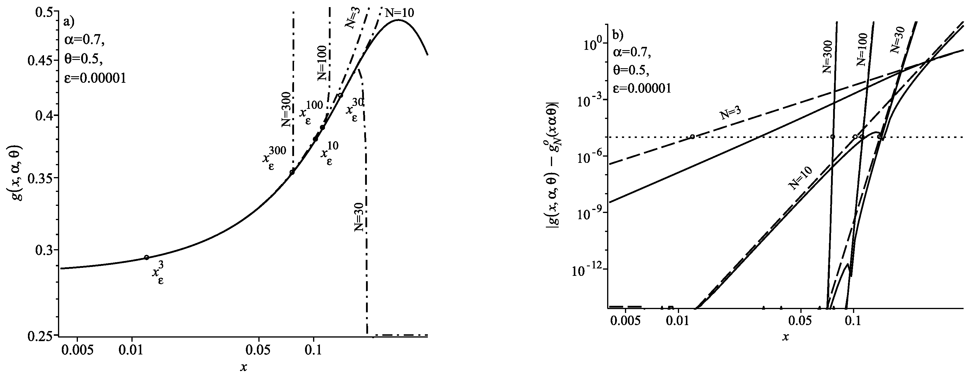
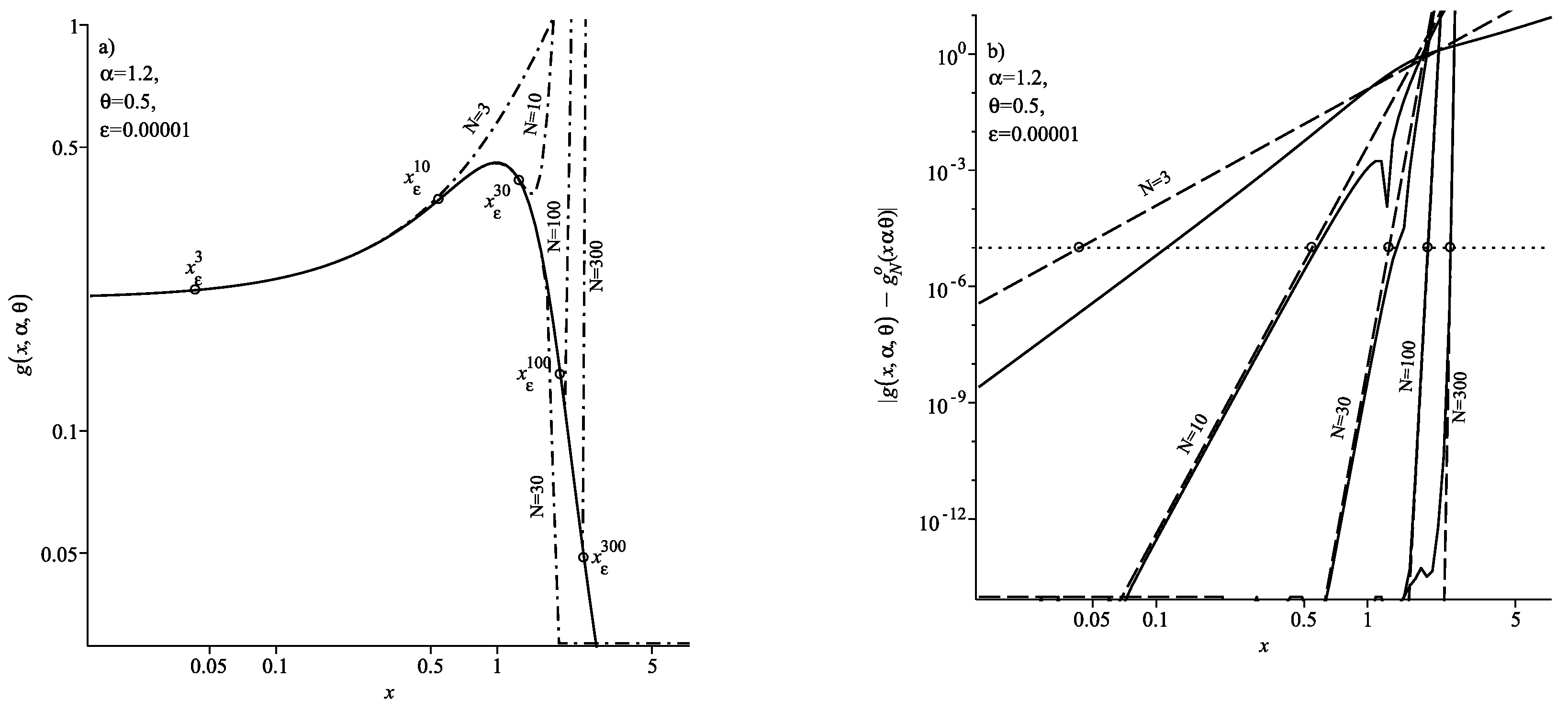
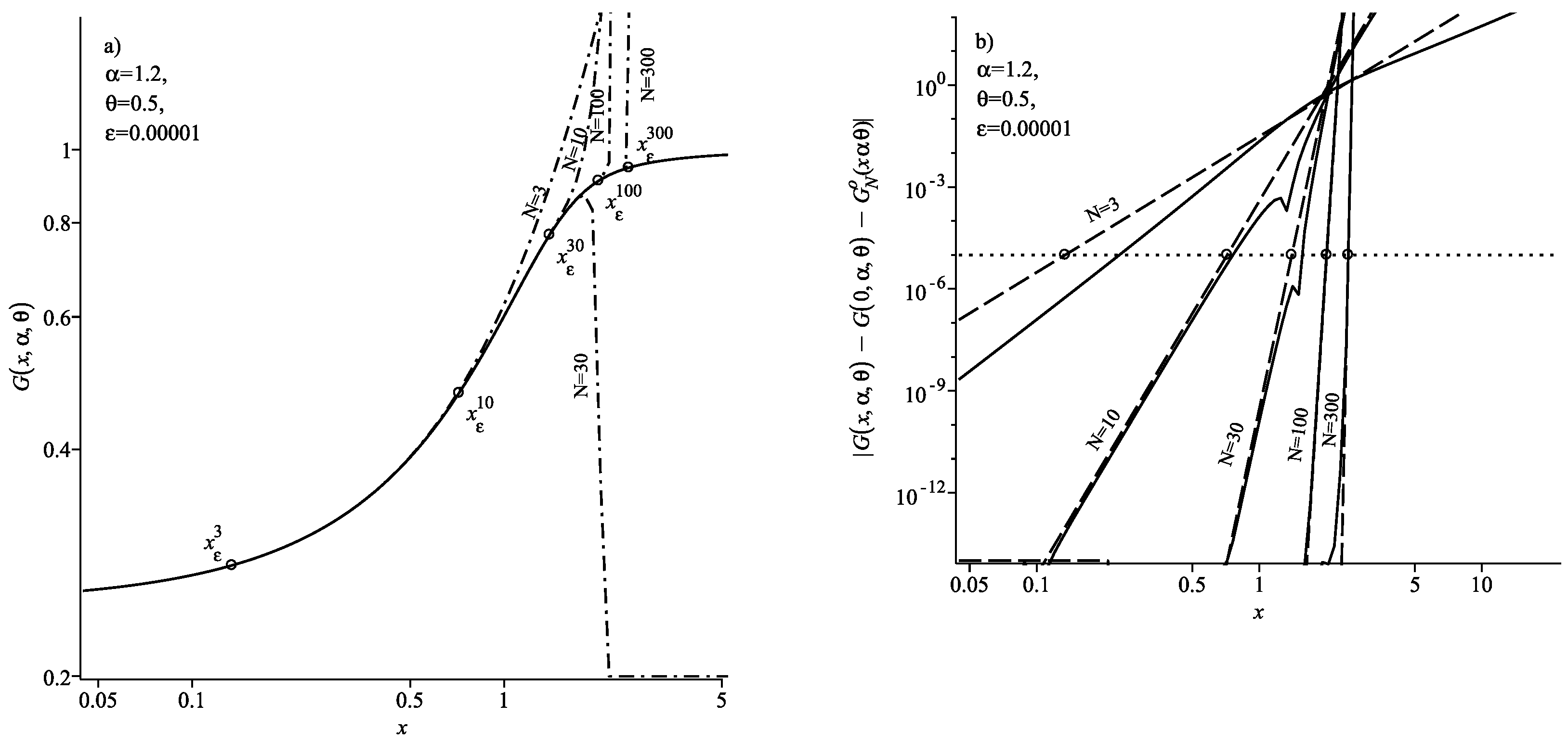
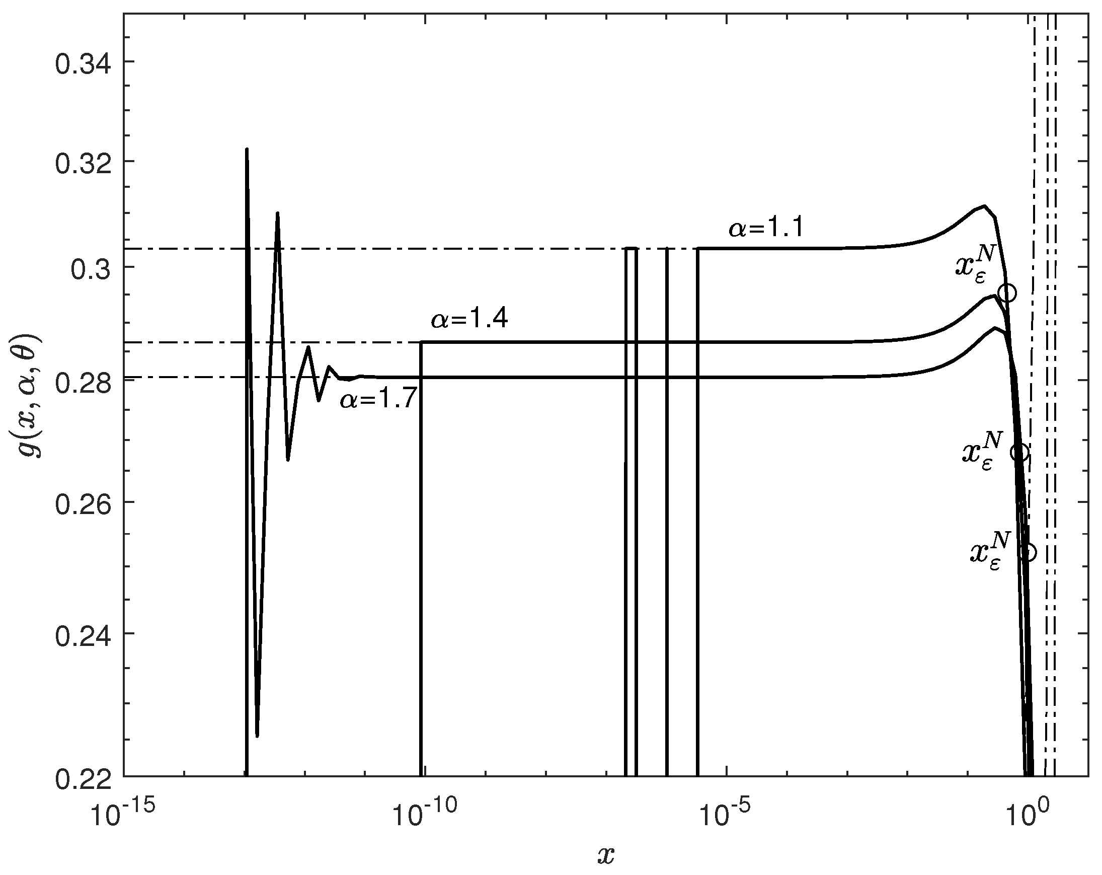
Figure 1a and Figure 2a show the results of calculating the probability density $g(x,\alpha ,\theta )$ using the series (12). In these figures, the solid curve corresponds to the exact density values $g(x,\alpha ,\theta )$ calculated with the help of (3) and the dash-dotted curves correspond to the density calculation results using the series (12) for the specified values of N. Figure 1b and Figure 2b show the results of the calculation of the absolute error $|g(x,\alpha ,\theta )-g_N^0(x,\alpha ,\theta )|$. In these figures, the solid curves correspond to the exact value of the absolute error $|g(x,\alpha ,\theta )-g_N^0(x,\alpha ,\theta )|$ where $g(x,\alpha ,\theta )$—the exact density value calculated when using (3), $g_N^0(x,\alpha ,\theta )$—for series (12) and the dashed curve corresponds to the estimate of the remainder term (13). The calculation results are given for the specified values of N in the figures. In all these figures, the circles show the position of the threshold coordinate $x_{\epsilon }^N$ for the selected level of accuracy $\epsilon$ and each number of summands N. It is clear from Figure 1b and Figure 2b that in the region $\left|x\right|⩽x_{\epsilon }^N$ the absolute magnitude of the error does not exceed the specified level of accuracy $\epsilon$ for all N. This means that at $\left|x\right|⩽x_{\epsilon }^N$ the expansion (12) can be used to calculate the density.

Corollary 1 shows that in the case $\alpha <1$, the series (12) is divergent at $N\to \infty$, and in the case $\alpha >1$, this series converges. The cause of this behavior lies in the ratio $\mathsf{\Gamma }\left(\right(n+1)/\alpha )/\mathsf{\Gamma }(n+1)$, which is present in this series. At $\alpha <1$, this ratio turns out to be more than unity and, as n increases, this ratio only rises. Therefore, to achieve the specified calculation accuracy $\epsilon$ one has to decrease the value of x. This can clearly been seen from the behavior of the threshold coordinates $x_{\epsilon }^N$. Figure 1a,b show that the addition of summands in the expansion (12) first leads to an increase in the range of x for which the inequality $\left|g\right(x,\alpha ,\theta -g_N^0(x,\alpha ,\theta )\left)\right|⩽\epsilon$ is satisfied. The fact that $x_{\epsilon }^3<x_{\epsilon }^{10}<x_{\epsilon }^{30}$ evidences this. However, further addition of summands leads to an increase in the ratio $\mathsf{\Gamma }\left(\right(n+1)/\alpha )/\mathsf{\Gamma }(n+1)$ and, thus, an increase in the absolute calculation error. Therefore, to achieve the specified level of accuracy, it is necessary to decrease the value of the coordinate x. This causes the threshold coordinate $x_{\epsilon }^N$ to start decreasing and we see that $x_{\epsilon }^{100}>x_{\epsilon }^{300}$.

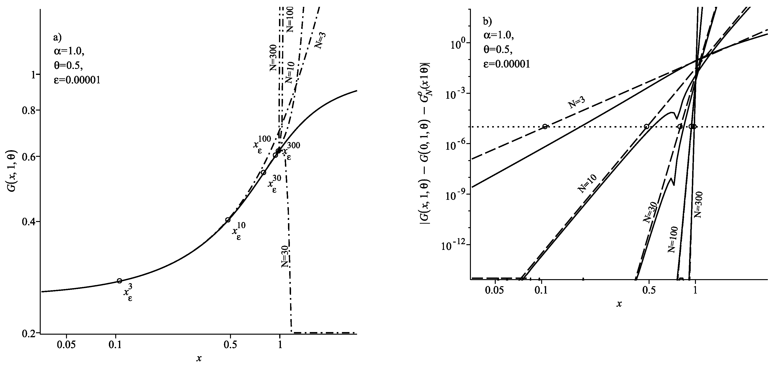
In the case $\alpha >1$, the situation changes. In this case, the ratio $\mathsf{\Gamma }\left(\right(n+1)/\alpha )/\mathsf{\Gamma }(n+1)<1$, and as n increases, this ratio only decreases. Consequently, the increase in the number of summands in (12) increases the accuracy of the density calculation. This leads to the fact that the range of values of x, for which the condition $|g(x,\alpha ,\theta )-g_N^0(x,\alpha ,\theta )|⩽\epsilon$ is met increases with the addition of the number of summands N in the sum (12). This is clearly seen from the location of the threshold coordinates $x_{\epsilon }^N$, shown in Figure 2a,b. We can see from the figures that $x_{\epsilon }^3<x_{\epsilon }^{10}<x_{\epsilon }^{30}<x_{\epsilon }^{100}<x_{\epsilon }^{300}$. Thus, in the case $\alpha >1$, the series (12) is convergent for all x at $N\to \infty$.

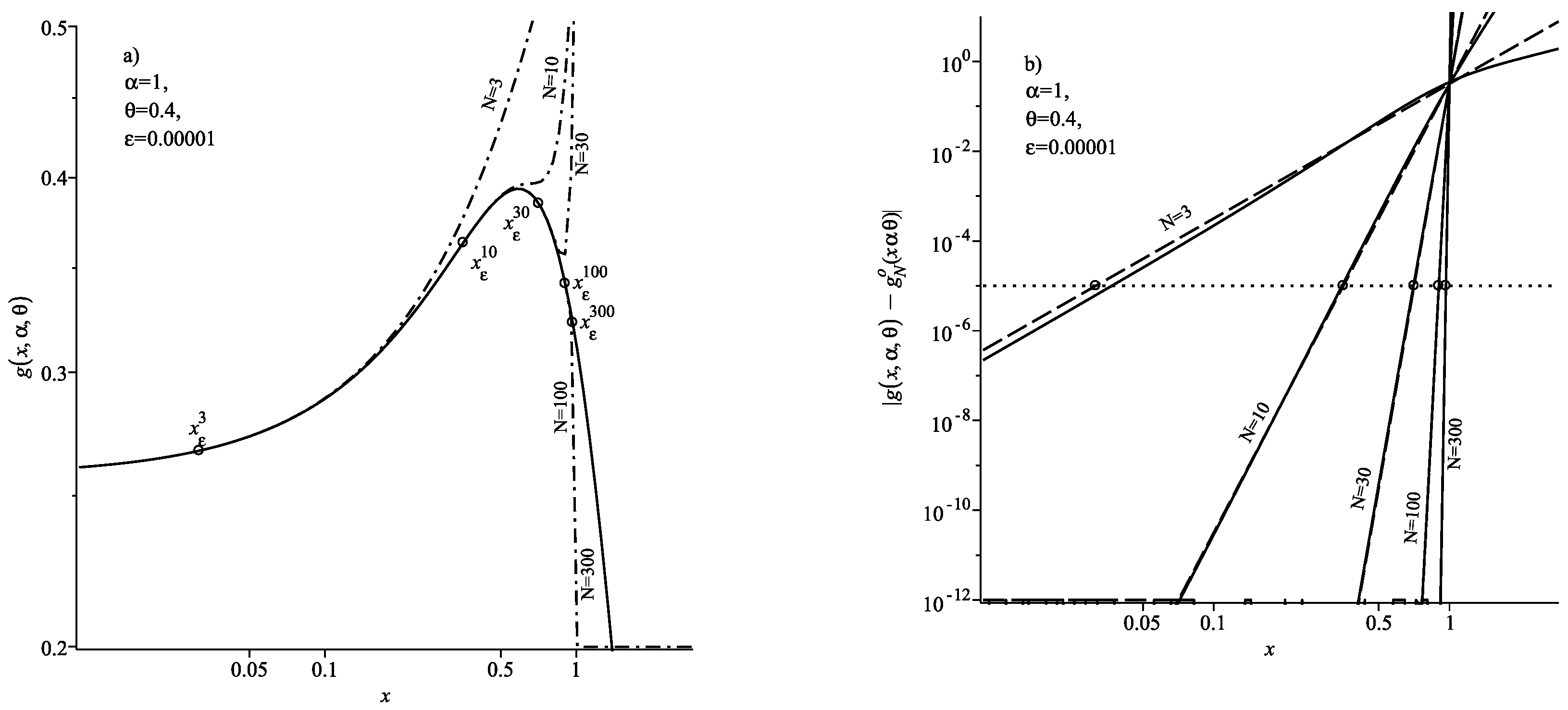
The results of calculations for the case $\alpha =1$ are given in Figure 3. This figure shows $x_{\epsilon }^3<x_{\epsilon }^{10}<x_{\epsilon }^{30}<x_{\epsilon }^{100}<x_{\epsilon }^{300}$. Thus, an increase in the number of summands N in the sum (12) leads to an increase in the interval x, within which the relation $|g(x,\alpha ,\theta )-g_N^0(x,\alpha ,\theta )|⩽\epsilon$ is satisfied. Here Formula (5) was used to calculate the density. It can also be observed from the figure that for all presented N at $x\to 1$, the partial sums of the series diverge. This is in full agreement with the statement of Corollary 1, which states that in the case $\alpha =1$, the series (12) converges at $\left|x\right|<1$.

4. Representation of the Distribution Function in the Form of a Power Series

Now we will try to obtain the representation of the distribution function in the case $x\to 0$ in the form of a power series. We will formulate the result obtained as a theorem.

Theorem 2.

In the case $x\to 0$ for any admissible set of parameters $(\alpha ,\theta )$, except for the values $\alpha =1,\theta =\pm 1$ for the distribution function $G(x,\alpha ,\theta )$, a representation in the form of a power series is valid.

$$G(x,\alpha ,\theta )=\frac{1-\theta }{2}+G_N^0(x,\alpha ,\theta )+{\mathcal{R}}_N^0(x,\alpha ,\theta ),x\to 0$$

(37)

where

$$\begin{array}{cc}\hfill G_N^0(x,\alpha ,\theta )& =\frac{1}{\pi \alpha }\sum _{n=0}^{N-1}\frac{x^{n+1}}{(n+1)!}\mathsf{\Gamma }\left(\frac{n+1}{\alpha }\right)\sin \left(\frac{\pi }{2}(n+1)(1-\theta )\right),\hfill \end{array}$$

(38)

$$\begin{array}{cc}\hfill |{\mathcal{R}}_n^0(x,\alpha ,\theta )|& ⩽\frac{{\left|x\right|}^{N+1}}{\alpha \pi (N+1)!}\mathsf{\Gamma }\left(\frac{N+1}{\alpha }\right).\hfill \end{array}$$

(39)

Proof. 

From the definition of the distribution function, it follows

$$G(x,\alpha ,\theta )-G(0,\alpha ,\theta )={\int }_0^{x}g(\xi ,\alpha ,\theta )d\xi .$$

Here $G(0,\alpha ,\theta )$ is the value of the distribution function in the point $x=0$ and is determined by Formula (9). Using the expansion (14) for the density $g(x,\alpha ,\theta )$ we obtain

$$G(x,\alpha ,\theta )=\frac{1-\theta }{2}+G_N^0(x,\alpha ,\theta )+{\mathcal{R}}_N^0(x,\alpha ,\theta ),x\to 0$$

(40)

where

$$\begin{array}{cc}\hfill G_N^0(x,\alpha ,\theta )& ={\int }_0^x{g}_N^0(\xi ,\alpha ,\theta )d\xi ,\hfill \end{array}$$

(41)

$$\begin{array}{cc}\hfill {\mathcal{R}}_N^0(x,\alpha ,\theta )& ={\int }_0^x{R}_n^0(\xi ,\alpha ,\theta )d\xi .\hfill \end{array}$$

(42)

Here $g_N^0(x,\alpha ,\theta )$ and $R_N^0(x,\alpha ,\theta )$ are determined by expressions (12) and (16), respectively.

To calculate the partial sum $G_N^0(x,\alpha ,\theta )$ we will make use of the results of theorem 1. It was obtained in this theorem that the partial sum $g_N^0(x,\alpha ,\theta )$ has the form (12). Substituting expression (12) in (41) and changing the order of integration and summation, we obtain

$$\begin{array}{c}{G}_N^0(x,\alpha ,\theta )=\frac{1}{\pi \alpha }\sum _{n=0}^{N-1}\frac{1}{n!}\mathsf{\Gamma }\left(\frac{n+1}{\alpha }\right)\sin \left(\frac{\pi }{2}(n+1)(1-\theta )\right){\int }_0^x{\xi }^{k}d\xi \hfill \\ \hfill =\frac{1}{\pi \alpha }\sum _{n=0}^{N-1}\frac{x^{n+1}}{(n+1)!}\mathsf{\Gamma }\left(\frac{n+1}{\alpha }\right)\sin \left(\frac{\pi }{2}(n+1)(1-\theta )\right).\end{array}$$

(43)

Now we obtain the expression for the remainder ${\mathcal{R}}_N^0(x,\alpha ,\theta )$. Substituting expression (16) in (42) and changing the order of integration, we obtain

$$\begin{array}{c}{\mathcal{R}}_N^0(x,\alpha ,\theta )={\int }_0^x{R}_N^0(\xi ,\alpha ,\theta )d\xi =\frac{1}{\pi }\Re {\int }_0^{\infty }\exp \left\{-t^{\alpha }\exp \left\{i\frac{\pi }{2}\alpha \theta \right\}\right\}dt{\int }_0^x{R}_N\left(it\xi \right)d\xi =\hfill \\ \hfill \frac{1}{\pi }\Re {\int }_0^{\infty }\exp \left\{-t^{\alpha }\exp \left\{i\frac{\pi }{2}\alpha \theta \right\}\right\}\frac{{\left(it\right)}^N}{N!}{\int }_0^x{\xi }^N{e}^{it\xi \zeta }d\xi ,\end{array}$$

where $0<\zeta <1$. This integral cannot be calculated directly, as the exact value of $\zeta$ is not known. It is only known that $\zeta \in (0,1)$. However, one can obtain an estimate of this integral.

To obtain an estimate for the integral, we use the inequality $\left|{\int }_0^x{\xi }^N{e}^{it\xi \zeta }d\xi \right|⩽\left|{\int }_0^x{\xi }^{N}d\xi \right|$. As a result, we obtain

$$\begin{array}{c}|{\mathcal{R}}_N^0(x,\alpha ,\theta )|=\frac{1}{\pi }\left|\Re {\int }_0^{\infty }\exp \left\{-t^{\alpha }\exp \left\{i\frac{\pi }{2}\alpha \theta \right\}\right\}\frac{{\left(it\right)}^N}{N!}{\int }_0^x{\xi }^N{e}^{it\xi \zeta }d\xi ,\right|\hfill \\ ⩽\frac{1}{\pi N!}\left|\Re i^N{\int }_0^{\infty }\exp \left\{-t^{\alpha }\exp \left\{i\frac{\pi }{2}\alpha \theta \right\}\right\}{t}^N{\int }_0^x{\xi }^{N}d\xi \right|\\ =\frac{1}{\pi (N+1)!}\left|\Re i^N{\int }_0^{\infty }\exp \left\{-t^{\alpha }\exp \left\{i\frac{\pi }{2}\alpha \theta \right\}\right\}{t}^N{x}^{N+1}\right|\\ ⩽\frac{{\left|x\right|}^{N+1}}{\alpha \pi (N+1)!}\left|\Re i^N{\int }_0^{\infty }\exp \left\{-\tau \exp \left\{i\frac{\pi }{2}\alpha \theta \right\}\right\}{\tau }^{\frac{N+1}{\alpha }-1}d\tau \right|\\ =\frac{{\left|x\right|}^{N+1}}{\alpha \pi (N+1)!}\mathsf{\Gamma }\left(\frac{N+1}{\alpha }\right)\left|\Re i^N\exp \left\{-i\frac{\pi }{2}\theta (N+1)\right\}\right|\\ \hfill ⩽\frac{{\left|x\right|}^{N+1}}{\alpha \pi (N+1)!}\mathsf{\Gamma }\left(\frac{N+1}{\alpha }\right).\end{array}$$

(44)

Here, to calculate the outer integral, the integration variable $t^{\alpha }=\tau$ was first substituted, and then Formula (10) was used. It should be noted that the case $\alpha =1$, $\theta =\pm 1$ must be excluded from consideration. Indeed, for such parameter values, the argument $\frac{\pi }{2}\alpha \theta =\pm \frac{\pi }{2}$ and integral (10) will diverge. Substituting expressions (43) and (44) in (43) we now get the statement of the theorem. □

The proven theorem shows that in the vicinity of the point $x=0$, the expansion (37) is valid for the distribution function of a strictly stable law with the characteristic function (1). However, as in the case of the probability density, the obtained power series diverges for all x at $\alpha <1$ and in the case $\alpha >1$ is convergent for all x. In the case $\alpha =1$, this series converges at $\left|x\right|<1$ and diverges at $\left|x\right|⩾1$. In this regard, for the values $\alpha <1$ the representation (37) is asymptotic, and for the values $\alpha >1$, the expansion $G(x,\alpha ,\theta )$ can be represented in the form of an infinite power series. We formulate this result as a corollary.

Corollary 2.

In the case $\alpha <1$, the series (38) diverges for all x at $N\to \infty$. In this case, the asymptotic expansion is valid for the distribution function $G(x,\alpha ,\theta )$ for any admissible θ

$$G(x,\alpha ,\theta )\sim \frac{1-\theta }{2}+\frac{1}{\pi \alpha }\sum _{n=0}^{N-1}\frac{x^{n+1}}{(n+1)!}\mathsf{\Gamma }\left(\frac{n+1}{\alpha }\right)\sin \left(\frac{\pi }{2}(n+1)(1-\theta )\right),x\to 0.$$

In the case $\alpha =1$, the series (37) converges at $\left|x\right|<1$. In this case, the distribution function $G(x,1,\theta )$ for any $\theta \ne \pm 1$ can be represented as an infinite series

$$G(x,1,\theta )=\frac{1-\theta }{2}+\frac{1}{\pi }\sum _{n=0}^{\infty }\frac{x^{n+1}}{n+1}\sin \left(\frac{\pi }{2}(n+1)(1-\theta )\right).$$

(45)

In the case $\alpha >1$, the series (38) at $N\to \infty$ converges for any x. In this case, the representation in the form of an infinite power series is true for the distribution function $G(x,\alpha ,\theta )$ for any admissible θ

$$G(x,\alpha ,\theta )=\frac{1-\theta }{2}+\frac{1}{\pi \alpha }\sum _{n=0}^{\infty }\frac{x^{n+1}}{(n+1)!}\mathsf{\Gamma }\left(\frac{n+1}{\alpha }\right)\sin \left(\frac{\pi }{2}(n+1)(1-\theta )\right).$$

Proof. 

We examine the convergence of the series (38). It is clear that this series is a sign-alternating series. Consequently,

$$\begin{array}{c}{G}_N^0(x,\alpha ,\theta )⩽\left|G_N^0(x,\alpha ,\theta )\right|⩽\frac{1}{\pi \alpha }\sum _{n=0}^{N-1}\frac{{\left|x\right|}^{n+1}}{(n+1)!}\mathsf{\Gamma }\left(\frac{n+1}{\alpha }\right)\left|\sin \left(\frac{\pi }{2}(n+1)(1-\theta )\right)\right|\hfill \\ \hfill ⩽\frac{1}{\pi \alpha }\sum _{n=0}^{N-1}\frac{{\left|x\right|}^{n+1}}{(n+1)!}\mathsf{\Gamma }\left(\frac{n+1}{\alpha }\right).\end{array}$$

We apply the Cauchy criterion in the limiting form to the obtained series. Using Stirling’s formula (23) and taking into consideration that $n+2\approx n+1$ at $n\to \infty$, we obtain

$$\begin{array}{c}\underset{n\to \infty }{\lim }{\left(\frac{{\left|x\right|}^{n+1}}{\alpha \pi }\frac{\mathsf{\Gamma }\left(\frac{n+1}{\alpha }\right)}{(n+1)!}\right)}^{1/n}=\underset{n\to \infty }{\lim }{\left(\frac{{\left|x\right|}^{n+1}}{\alpha \pi }\frac{\mathsf{\Gamma }\left(\frac{n+1}{\alpha }\right)}{\mathsf{\Gamma }(n+2)}\right)}^{1/n}\hfill \\ =\underset{n\to \infty }{\lim }\frac{{\left|x\right|}^{1+\frac{1}{n}}}{{\left(\alpha \pi \right)}^{1/n}}\frac{{\left(\exp \left\{-\frac{n+1}{\alpha }\right\}{\left(\frac{n+1}{\alpha }\right)}^{\frac{n+1}{\alpha }-\frac{1}{2}}\sqrt{2\pi }\right)}^{\frac{1}{n}}}{{\left(\exp \left\{-(n+2)\right\}{(n+2)}^{n+2-\frac{1}{2}}\sqrt{2\pi }\right)}^{\frac{1}{n}}}=\\ \underset{n\to \infty }{\lim }\frac{{\left|x\right|}^{1+\frac{1}{n}}}{{\left(\alpha \pi \right)}^{1/n}}\frac{\exp \left\{-\frac{1}{\alpha }\left(1+\frac{1}{n}\right)\right\}{\left(\frac{n+1}{\alpha }\right)}^{\frac{1}{\alpha }\left(1+\frac{1}{n}\right)-\frac{1}{2n}}}{\exp \left\{-1-\frac{1}{2n}\right\}{(n+2)}^{1-\frac{3}{2n}}}=\underset{n\to \infty }{\lim }\left|x\right|e^{1-\frac{1}{\alpha }}{\alpha }^{-\frac{1}{\alpha }}\frac{{(n+1)}^{\frac{1}{\alpha }}}{n+2}\\ \hfill =\underset{n\to \infty }{\lim }\left|x\right|e^{1-\frac{1}{\alpha }}{\alpha }^{-\frac{1}{\alpha }}{(n+1)}^{\frac{1}{\alpha }-1}=\left\{\begin{array}{cc}\infty ,& \alpha <1,\\ \left|x\right|,& \alpha =1,\\ 0,& \alpha >1.\end{array}\right.\end{array}$$

This shows that in the case $\alpha <1$, the series (38) diverges for all x; in the case $\alpha >1$, the series converges for all x, and in the case $\alpha =1$ the series (38) converges if $\left|x\right|<1$.

Now we consider the case $\alpha <1$. In this case, the series (38) diverges at $N\to \infty$. However, it follows from expression (39) that for some fixed N

$${\mathcal{R}}_N^0(x,\alpha ,\theta )=O\left(x^{N+1}\right),x\to 0.$$

Consequently, for each N we have

$$G(x,\alpha ,\theta )=\frac{1-\theta }{2}+\frac{1}{\pi \alpha }\sum _{n=0}^{N-1}\frac{x^{n+1}}{(n+1)!}\mathsf{\Gamma }\left(\frac{n+1}{\alpha }\right)\sin \left(\frac{\pi }{2}(n+1)(1-\theta )\right)+O\left(x^{N+1}\right),x\to 0.$$

Thus, we have obtained the definition of an asymptotic series. Consequently,

$$G(x,\alpha ,\theta )\sim \frac{1-\theta }{2}+\frac{1}{\pi \alpha }\sum _{n=0}^{N-1}\frac{x^{n+1}}{(n+1)!}\mathsf{\Gamma }\left(\frac{n+1}{\alpha }\right)\sin \left(\frac{\pi }{2}(n+1)(1-\theta )\right),x\to 0,\alpha <1.$$

Now we consider the case $\alpha >1$. In this case, the series (38) is convergent. It follows from expressions (37) and (39) that

$$\left|G(x,\alpha ,\theta )-(1-\theta )/2-G_N^0(x,\alpha ,\theta )\right|⩽\frac{{\left|x\right|}^{N+1}}{\alpha \pi (N+1)!}\mathsf{\Gamma }\left(\frac{N+1}{\alpha }\right).$$

(46)

We will find the limit at $N\to \infty$ of the right-hand side of this inequality. Using Stirling’s Formula (23) and taking into account that $N+2\approx N+1$ at $N\to \infty$, we obtain

$$\begin{array}{c}\frac{1}{\alpha \pi }\underset{N\to \infty }{\lim }\frac{\mathsf{\Gamma }\left(\frac{N+1}{\alpha }\right)}{(N+1)!}{\left|x\right|}^{N+1}=\frac{1}{\alpha \pi }\underset{N\to \infty }{\lim }\frac{\mathsf{\Gamma }\left(\frac{N+1}{\alpha }\right)}{\mathsf{\Gamma }(N+2)}{\left|x\right|}^{N+1}\hfill \\ =\frac{1}{\alpha \pi }\underset{N\to \infty }{\lim }\frac{e^{-\frac{N+1}{\alpha }}{\left(\frac{N+1}{\alpha }\right)}^{\frac{N+1}{\alpha }-\frac{1}{2}}\sqrt{2\pi }}{e^{-(N+2)}{(N+2)}^{N+2-1/2}\sqrt{2\pi }}{\left|x\right|}^{N+1}=\frac{1}{\alpha \pi }\underset{N\to \infty }{\lim }\frac{e^{-\frac{N+1}{\alpha }}{\left(\frac{N+1}{\alpha }\right)}^{\frac{N+1}{\alpha }-\frac{1}{2}}}{e^{-(N+1)}{(N+1)}^{N+1-1/2}}{\left|x\right|}^{N+1}\\ =\frac{{\alpha }^{-\frac{1}{2}-\frac{1}{\alpha }}}{\pi }\underset{N\to \infty }{\lim }{\alpha }^{-\frac{N}{\alpha }}{e}^{(N+1)\left(1-\frac{1}{\alpha }\right)}{(N+1)}^{(N+1)\left(\frac{1}{\alpha }-1\right)}{\left|x\right|}^{N+1}=\\ \frac{{\alpha }^{-\frac{1}{2}-\frac{1}{\alpha }}}{\pi }\underset{N\to \infty }{\lim }\exp \left\{(N+1)\left(1-\frac{1}{\alpha }\right)(1-\ln (N+1))-\frac{N}{\alpha }\ln \alpha \right\}{\left|x\right|}^{N+1}\\ \hfill =\left\{\begin{array}{cc}\infty ,& \alpha <1,\\ 0,& \alpha >1,\\ 0,& \alpha =1,\left|x\right|<1,\\ \infty ,& \alpha =1,\left|x\right|⩾1.\end{array}\right.\end{array}$$

Thus, in the two cases $\alpha >1$ and $\alpha =1,\left|x\right|<1$, the right side of the inequality (46) is an element of an infinitesimal sequence. In turn, this means that in the above two cases, for any fixed x, the sequences $(1-\theta )/2+G_N^0(x,\alpha ,\theta )$ converge to the distribution function $G(x,\alpha ,\theta )$. Therefore, in the considered case $\alpha >1$ for any fixed x the distribution function can be represented as an infinite series.

$$G(x,\alpha ,\theta )=\frac{1-\theta }{2}+\frac{1}{\pi \alpha }\sum _{n=0}^{\infty }\frac{x^{n+1}}{(n+1)!}\mathsf{\Gamma }\left(\frac{n+1}{\alpha }\right)\sin \left(\frac{\pi }{2}(n+1)(1-\theta )\right).$$

Now we consider the case $\alpha =1$. As shown above, in this case, when the condition $\left|x\right|<1$ is met, the right side (46) is an element of an infinitesimal series. Therefore, for any fixed $\left|x\right|<1$ the representation in the form of an infinite series is true for the distribution function

$$G(x,1,\theta )=\frac{1-\theta }{2}+\frac{1}{\pi \alpha }\sum _{n=0}^{\infty }\frac{x^{n+1}}{(n+1)}\sin \left(\frac{\pi }{2}(n+1)(1-\theta )\right).$$

Thus, the corollary has been proven completely. □

As in the case of the probability density, the proven property shows that in the case $\alpha =1$ and $\left|x\right|<1$, the series (45) converges to the distribution function $G(x,1,\theta )$. It is possible to show that this series converges to the distribution function (8). We will formulate this result as a remark.

Remark 2.

In the case $\alpha =1$ for any $-1<\theta <1$ in the region $-1<x<1$, the series (45) converges to the distribution function (8).

Proof. 

To prove this remark, we proceed in the same way as in the proof of remark 1. Let us show that the expansion of the distribution function (8) into a Taylor series in the vicinity of the point $x=0$ has the form (45). We will use the reduction formulas $\cos \left(\frac{\pi }{2}\theta \right)=\sin \left(\frac{\pi }{2}(1-\theta )\right)$ and $\sin \left(\frac{\pi }{2}\theta \right)=\cos \left(\frac{\pi }{2}(1-\theta )\right)$, and we will write the distribution function (8) in the form

$$G(x,1,\theta )=\frac{1}{2}+\frac{1}{\pi }\arctan \left(\frac{x-\cos \left(\frac{\pi }{2}(1-\theta )\right)}{\sin \left(\frac{\pi }{2}(1-\theta )\right)}\right).$$

Note that the function $\arctan \left(x\right)$ is infinitely differentiable, therefore, expanding it into an infinite series, we obtain

$$G(x,1,\theta )=G(0,1,\theta )+\sum _{n=1}^{\infty }\frac{1}{n!}{\left.\frac{d^{n}G(x,1,\theta )}{d{x}^n}\right|}_{x=0}{x}^n.$$

(47)

For the derivative of the order n we have

$$\begin{array}{c}\frac{d^{n}G(x,1,\theta )}{d{x}^n}=\frac{d^{n-1}}{d{x}^{n-1}}\frac{dG(x,1,\theta )}{dx}=\frac{1}{\pi }\frac{d^{n-1}}{d{x}^{n-1}}\frac{1}{1+{\left(\frac{x-\cos \left(\frac{\pi }{2}(1-\theta )\right)}{\sin \left(\frac{\pi }{2}(1-\theta )\right)}\right)}^2}\frac{1}{\sin \left(\frac{\pi }{2}(1-\theta )\right)}=\hfill \\ \hfill \frac{1}{\pi }\frac{d^{n-1}}{d{x}^{n-1}}\frac{\sin \left(\frac{\pi }{2}(1-\theta )\right)}{x^2-2x\cos \left(\frac{\pi }{2}(1-\theta )\right)+1}=\frac{d^{n-1}g(x,1,\theta )}{d{x}^{n-1}}.\end{array}$$

(48)

Thus, the problem has been reduced to calculating the derivative $n-1$ of the probability density $g(x,1,\theta )$. However, this problem has been solved by us when proving Remark 1. Using Formula (33), we get

$$\begin{array}{c}\frac{d^{n-1}g(x,1,\theta )}{d{x}^{n-1}}=\hfill \\ \hfill \frac{\sin \left(\frac{\pi }{2}(1-\theta )\right)}{\pi }\sum _{k=0}^{\left[\frac{n-1}{2}\right]}\frac{{(-1)}^{n-k-1}(n-1)!(n-k-1)!}{k!(n-2k-1)!}\frac{{\left(2x-2\cos \left(\frac{\pi }{2}(1-\theta )\right)\right)}^{n-2k-1}}{{\left(x^2-2x\cos \left(\frac{\pi }{2}(1-\theta )\right)+1\right)}^{n-k}}\end{array}$$

Substituting this expression in (48) and calculating the value of the obtained derivative in the point $x=0$ and then using (35), we obtain

$$\begin{array}{c}{\left.\frac{d^{n}G(x,1,\theta )}{d{x}^n}\right|}_{x=0}=\hfill \\ \frac{\sin \left(\frac{\pi }{2}(1-\theta )\right)}{\pi }\sum _{k=0}^{\left[\frac{n-1}{2}\right]}\frac{{(-1)}^k(n-1)!(n-k-1)!}{k!(n-2k-1)!}{\left(2\cos \left(\frac{\pi }{2}(1-\theta )\right)\right)}^{n-2k-1}\\ \hfill =\frac{1}{\pi }(n-1)!\sin \left(\frac{\pi }{2}n(1-\theta )\right),\end{array}$$

where it was taken into account that ${(-1)}^{2n-2-3k}={(-1)}^k$.

Substituting now the obtained expression for the n-th derivative in (47) and taking into consideration (9), we get

$$\begin{array}{c}G(x,1,\theta )=\frac{1}{2}(1-\theta )+\frac{1}{\pi }\sum _{n=1}^{\infty }\frac{x^n}{n}\sin \left(\frac{\pi }{2}n(1-\theta )\right)\hfill \\ \hfill =\frac{1}{2}(1-\theta )+\frac{1}{\pi }\sum _{k=0}^{\infty }\frac{x^{k+1}}{k+1}\sin \left(\frac{\pi }{2}(k+1)(1-\theta )\right).\end{array}$$

Here, in the last equality, the summation index $n=k+1$ was changed. Thus, the expansion of the distribution function (8) into a Taylor series in the vicinity of the point $x=0$ exactly coincides with the series (45). This completely proves the remark. □

Theorem 2 provides an opportunity to find the range of values of the coordinate x within which the absolute error of calculating $G(x,\alpha ,\theta )$ using the expansion (37) will not exceed the prespecified value. Indeed, from (37) and (39) we have

$$\left|G(x,\alpha ,\theta )-\frac{1}{2}(1-\theta )-G_N^0(x,\alpha ,\theta )\right|⩽\frac{{\left|x\right|}^{N+1}}{\alpha \pi (N+1)!}\mathsf{\Gamma }\left(\frac{N+1}{\alpha }\right).$$

If we now set the absolute magnitude of the error for a specified fixed N as

$$\left|G(x,\alpha ,\theta )-\frac{1}{2}(1-\theta )-G_N^0(x,\alpha ,\theta )\right|=\epsilon ,$$

then it is possible to introduce the threshold coordinate

$$x_{\epsilon }^N={\left(\frac{\pi \epsilon \alpha (N+1)!}{\mathsf{\Gamma }\left(\frac{N+1}{\alpha }\right)}\right)}^{\frac{1}{N+1}}$$

(49)

This value shows that for all x satisfying the condition $\left|x\right|⩽x_{\epsilon }^N$, the absolute magnitude of the error in calculating the distribution function using the expansion (37) will not exceed the value $\epsilon$:

$$\left|G(x,\alpha ,\theta )-\frac{1}{2}(1-\theta )-G_N^0(x,\alpha ,\theta )\right|⩽\epsilon ,-x_{\epsilon }^N⩽x⩽x_{\epsilon }^N.$$

(50)

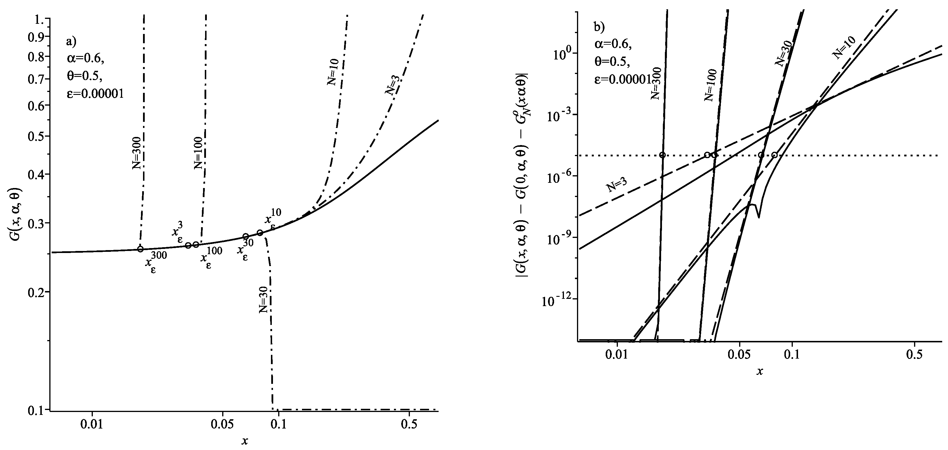
Figure 4a and Figure 5a show the calculation results of the distribution function using the integral representation (6) (solid curves) and using the expansion (37) (dash-dotted curves) for parameter values $\alpha =0.6$, $\theta =0.5$ and $\alpha =1.2$, $\theta =0.5$, respectively. These figures contain the results of calculating the distribution function using the expansion (37) for the values $N=3,10,30,100,300$. Figure 4b and Figure 5b show the results of calculating the absolute error. In these figures, the dashed curve corresponds to the estimate of the remainder (39), and the solid curves correspond the exact value of the absolute error $|G(x,\alpha ,\theta )-\frac{1}{2}(1-\theta )-G_N^0(x,\alpha ,\theta )\left)\right|$ for the values $N=3,10,30,100,300$. Here $G(x,\alpha ,\theta )$ is the exact value of the distribution function calculated using the representation (6), $G_N^0(x,\alpha ,\theta )$ is determined by (38).

From Figure 4b and Figure 5b it is clear that the condition (50) is met for all given values of N. In these figures, the location of the threshold coordinate $x_{\epsilon }^N$ is marked with circles and the dotted line corresponds to the specified level of accuracy $\epsilon$. We can see from the presented figures that for all values of x satisfying the condition $\left|x\right|⩽x_{\epsilon }^N$, both the estimate of the remainder (39) (dashed lines), and the exact value of the absolute error (solid curves) are below the specified level of accuracy $\epsilon$. This confirms the validity of the condition (50) and shows that Formula (49) can be used to estimate the boundary value of the coordinate in the expansion (37) at which the specified level of accuracy is achieved.

It should be noted that in the case $\alpha <1$ and $\alpha >1$, the threshold coordinate $x_{\epsilon }^N$ behaves differently as the number of summands N in the expansion (37) increases. In the case $\alpha <1$ (Figure 4), an increase in N first increases the threshold coordinate $x_{\epsilon }^N$ ($x_{\epsilon }^3<x_{\epsilon }^{10}$), but with further increase in N, the threshold coordinate $x_{\epsilon }^N$ decreases $(x_{\epsilon }^{30}>x_{\epsilon }^{100}>x_{\epsilon }^{300})$. The threshold coordinate $x_{\epsilon }^N$ behaves quite differently in the case $\alpha >1$. In this case, with an increase in N the value of the threshold coordinate increases: $x_{\epsilon }^3<x_{\epsilon }^{10}<x_{\epsilon }^{30}<x_{\epsilon }^{100}<x_{\epsilon }^{300}$ (see Figure 5). Such behavior of the threshold coordinate $x_{\epsilon }^N$ is due to the fact that in the case ($\alpha <1$) the series (38) is divergent, and in the case $\alpha >1$ this series converges (see Corollary 2).

In the case $\alpha =1$, the threshold coordinate behaves in the same way as the case $\alpha >1$. With an increase in the number of summands of N in the expansion (37) the value of the threshold coordinate $x_{\epsilon }^N$ increases. We can see this from Figure 6, which contains $x_{\epsilon }^3<x_{\epsilon }^{10}<x_{\epsilon }^{30}<x_{\epsilon }^{100}<x_{\epsilon }^{300}$. However, unlike the previous case, ${\lim }_{N\to \infty }{x}_{\epsilon }^N=1$. Indeed, in the case $\alpha =1$ Formula (49) takes the form $x_{\epsilon }^N={\left(\epsilon (N+1)\right)}^{1/(N+1)}$. Thus,

$$\underset{N\to \infty }{\lim }{x}_{\epsilon }^N=\underset{N\to \infty }{\lim }{\left(\epsilon (N+1)\right)}^{1/(N+1)}=\underset{N\to \infty }{\lim }\exp \left\{\frac{\ln \left(\epsilon \right(N+1\left)\right)}{N+1}\right\}=1.$$

Such behavior of the threshold coordinate $x_{\epsilon }^N$ is a consequence of the proven Corollary 2. Indeed, in the case $\alpha =1$ the series (38) and, therefore, the representation (37) converges in the region $\left|x\right|<1$.

The results of calculating the absolute error in the case $\alpha =1$ are given in Figure 6b. In this figure, the value of the threshold coordinate $x_{\epsilon }^N$ for different values N is shown with a circle. We can see from the presented results that for the values $\left|x\right|⩽x_{\epsilon }^N$ both the estimate of the remainder (39) (dashed lines), and the exact value of the absolute error (solid curves) turn out to be less than the specified accuracy level $\epsilon$ (dotted line). This demonstrates that the use of Formula (49) to estimate the values of the boundary coordinate leads to the validity of the condition (50).

5. Calculation of the Probability Density and Distribution Function for Small $\mathbf{X}$

We return to the problem of calculating the probability density of a strictly stable law. As mentioned in the introduction, the main approach to the calculation of the probability density is to use the integral representation. For a strictly stable law with the characteristic function (1), such an integral representation is determined by Formula (3). This formula is valid for any $x\ne 0$ and any admissible values of parameters $\alpha$ and $\theta$ except for $\alpha =1$. 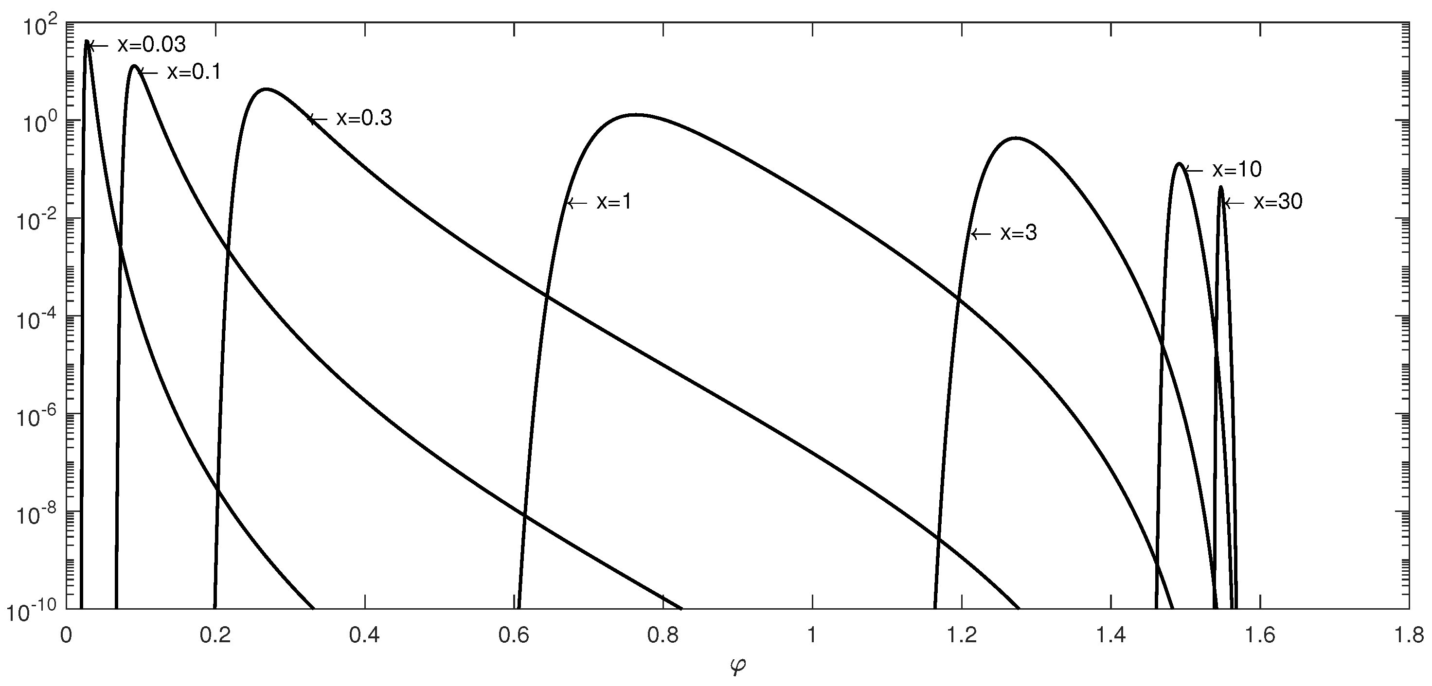However, in practice it is not possible to calculate the integral in (3) numerically for all values of x. The reason for this lies in the behavior of the integrand. Figure 7 shows the graph of the integrand in Formula (3) depending on the integration variable $\phi$ for different values of x. The graph of the function is plotted on a semi-logarithmic scale. We can see from this figure that as the value of x decreases, the integrand turns into a function with a very narrow and sharp peak. With a further decrease in x, this peak becomes even narrower and higher. The same behavior of the integrand is also observed for large values of x. This leads to the fact that for very small and for very large values of x numerical integration algorithms cannot calculate the integral of this function.

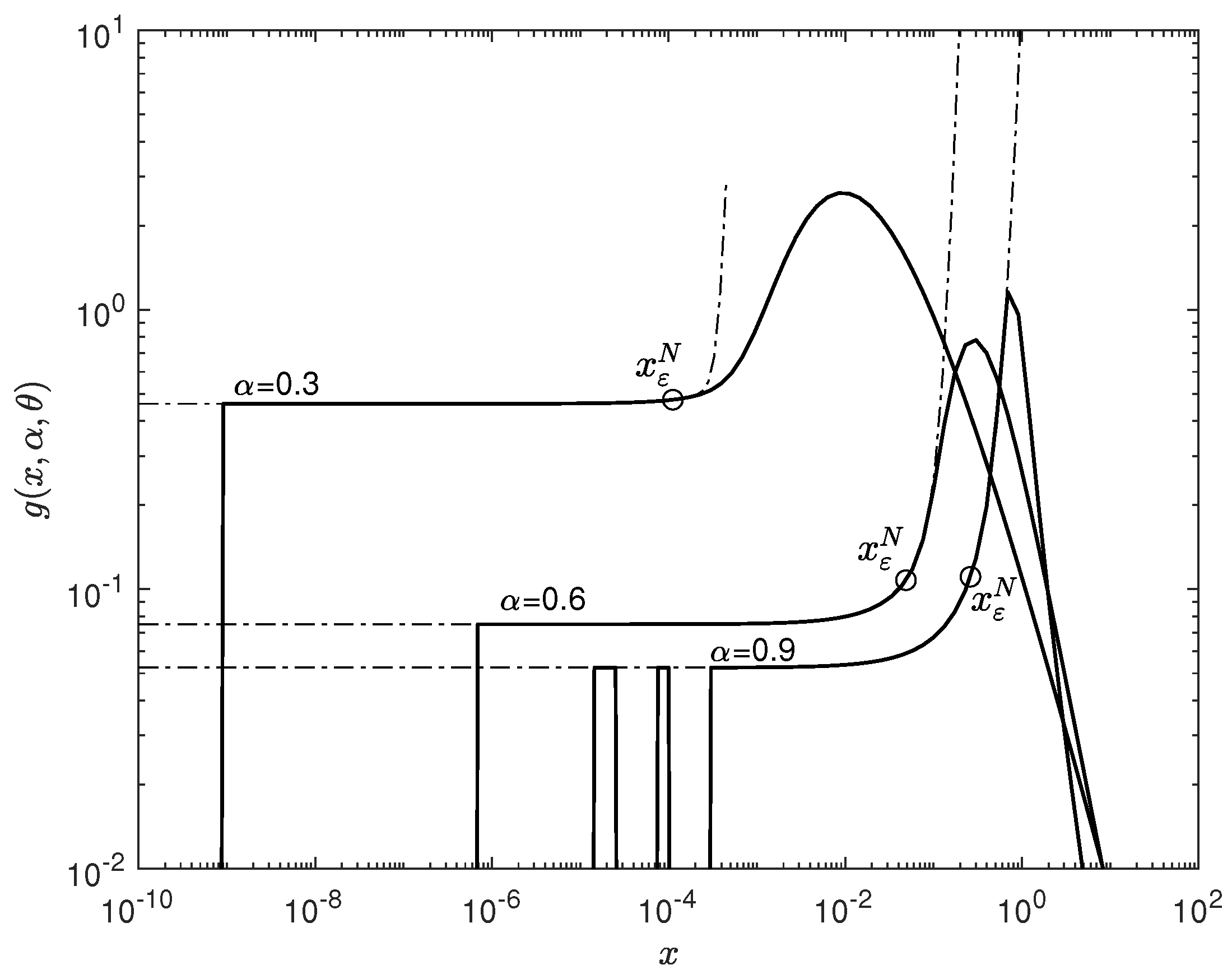
Figure 8 and Figure 9 show the results of calculating the probability density using the integral representation (3) (solid curves). Figure 8 shows the case $\alpha <1$, Figure 9 shows the case $\alpha >1$. The Gauss–Kronrod algorithm was used to calculate the integral in Formula (3). It is clear from the presented calculations that for small values of x the numerical integration method used cannot calculate the integral in (3). The critical value of the coordinate $x_{cr}$ at which the numerical integration algorithm used begins to produce an incorrect result for $\alpha =0.3$ is $x_{cr}\approx 9·{10}^{-10}$; for $\alpha =0.6$, it is $x_{cr}\approx 7·{10}^{-7}$; and for $\alpha =0.9$, it is $x_{cr}\approx 3·{10}^{-4}$ (see Figure 8). In the case $\alpha >1$ (see Figure 9), for the value $\alpha =1.1$, the critical value is $x_{cr}\approx 3·{10}^{-6}$, for the value $\alpha =1.4$, it is $x_{cr}\approx {10}^{-10}$; and for the value $\alpha =1.7$, it is $x_{cr}\approx {10}^{-11}$. Consequently, at $x<x_{cr}$ it is necessary to use other methods to calculate the probability density. The same problem exists for integral representations of the density of stable laws in other parameterizations of the characteristic function (see [14,16,18,19]). To solve this problem in these works, the authors used various numerical methods that make it possible to increase the accuracy of the calculation. However, these methods increase the accuracy of the calculations but do not solve the problem completely.

To calculate the density for the values $\left|x\right|<x_{cr}$, one should use other representations that do not have any singularities in this area. The most suitable option for this purpose is the power series representation obtained in Theorem 1 for the probability density. The estimate of the remainder (13) obtained in the same theorem make it possible to obtain the formula for the threshold coordinate $x_{\epsilon }^N$ (36) at which the given value of the absolute error $\epsilon$ is achieved for a fixed N. This means that in the region $-x_{\epsilon }^N⩽x⩽x_{\epsilon }^N$, the absolute error of the density calculation using the series (11) will not exceed the specified value $\epsilon$. In Figure 8 and Figure 9 the dash-dotted curves show the results of calculating the probability density using the series (12) for the specified values of $\alpha$. The position of the threshold coordinate $x_{\epsilon }^N$ is shown with circles. The values $x_{\epsilon }^N$ are calculated for the absolute error $\epsilon ={10}^{-5}$ and $N=10$. These figures show that, in the region $x_{cr}⩽x⩽x_{\epsilon }^N$, the results of calculating the probability density using the integral representation (3) and using the series (12) coincide. For the values $\left|x\right|⩽x_{cr}$, the numerical integration algorithm no longer allows for the obtainment of the correct density value. At the same time, the calculation of the probability density using the series (12) does not cause any difficulties. It follows that for the values $\left|x\right|⩽x_{\epsilon }^N$, it is expedient to use the series (12) to calculate the probability density. Thus, using theorem 1 and, in particular, the series(12), completely solves the problem of calculating the probability density at $x\to 0$.

Similar problems arise when calculating the distribution function using the integral representation (6). The integrand in this integral representation also has some singularities at $x\to 0$. In the general case, the integrand in (6) (see also (7)) behaves in the following way. In the point of the lower limit $\phi =-\pi \theta /2$, the integrand is equal to 1, and in the point of the upper limit $\phi =\pi /2$ the value of the integrand is equal to 0. As the variable $\phi$ increases from the value $-\pi \theta /2$ to the value $\pi /2$, the integrand decreases monotonically from 1 to 0. However, for very small values of x, the integrand in (7) decreases very sharply from 1 to 0 in a very narrow range $\phi$. As a result, some numerical integration algorithms cannot recognize such a sharp decrease in the function and will return an incorrect integration result. To exclude the possibility of incorrect results completely for small values x, it is expedient to use the expansion of the distribution function into a series obtained in Theorem 2. The estimate of the remainder obtained in this theorem make it possible to obtain Formula (49) for the threshold coordinate. The value $x_{\epsilon }^N$ enables us to determine the range of x at which the inequality (50) is satisfied. In other words, in the range of values $\left|x\right|⩽x_{\epsilon }^N$, the absolute error of calculating the distribution function using the expansion (37) will not exceed the value $\epsilon$ where $\epsilon$ is given in advance. Therefore, when calculating the distribution function in the range of values $\left|x\right|⩽x_{\epsilon }^N$, it is expedient to use the expansion (37), while for the range of values $\left|x\right|>x_{\epsilon }^N$, it is advantageous to use the integral representation (6).

6. Conclusions

The major approach to the calculation of the probability density and the distribution function of stable laws is the use of integral representations. Theoretically, these representations are valid for all values of the coordinate x. However, it is not possible to calculate the density numerically for all x. Problems arise in the domain of very small and very large values of x. Therefore, it is expedient to use other methods for numerical calculations.

This paper considers the problem of calculating the probability density and distribution function in the case of $x\to 0$ for a strictly stable law with a characteristic function (1). To solve this problem, expansions of the probability density and distribution function in a power series and estimates of the residual terms for each of the expansions were obtained. Estimates of the threshold coordinates $x_{\epsilon }^N$ were obtained for the expansion of the probability density and the distribution function, which are defined by expressions (36) and (49), respectively. The threshold coordinate allows one to determine the domain of coordinates $\left|x\right|⩽x_{\epsilon }^N$ within which the absolute computational error will not exceed the specified accuracy level $\epsilon$. The performed calculations showed that the value of the critical coordinate $x_{cr}$ at which the numerical integration algorithm used starts giving an incorrect result is significantly less than the threshold coordinate $x_{\epsilon }^N$ (see Figure 8 and Figure 9). This fact shows that in the domain $\left|x\right|⩽x_{\epsilon }^N$, it is possible to use Theorems 1 and 2 to calculate the probability density and distribution function.

The analysis of the obtained series made it possible to confirm both the known properties of these series and to establish new properties, as well as to improve the known estimates of the remainder terms. It was shown that in the case $\alpha <1$, the power series were divergent for any x at $N\to \infty$. In this case, these series are asymptotic at $x\to 0$. In the case $\alpha >1$, the obtained series are convergent for all admissible x. In this case, representations in the form of infinite series are valid for the probability density and distribution function (see Corollaries 1 and 2). These results are known and were previously obtained for the characteristic function in parameterization <<B>> in works [23,24] (see Chapter 17, §7), [1] (see §2.4 and §2.5), and [34] (see §4.2, §4.3). It can be shown that the expansions from Corollaries 1 and 2 in the cases $\alpha <1$ and $\alpha >1$ completely correspond to the expansions in the mentioned works. Examining the case $\alpha =1$ helped us in establishing that the expansions of the probability density and distribution function converged to the probability density (5) and the distribution function (8) in the domain $\left|x\right|<1$ for any $-1<\theta <1$ (see Remarks 1 and 2).

This paper improves the estimates of the remainder terms in the expansions of the probability density and the distribution function defined by the formulas (13) and (39). The estimate of the remainder term obtained earlier (see [1], formula (2.5.2)) refers to the expansion of the probability density in parameterization <<B>> and in the case of $\alpha <1$, it has the form

$$|R_N|⩽\frac{1}{\pi \alpha }\frac{\mathsf{\Gamma }\left(\frac{N+1}{\alpha }\right)}{N!}{\left(\cos \left(\frac{\pi }{2}\alpha \beta \right)\right)}^{-(N+1)/\alpha }.$$

(51)

We will take the relation $\theta =\beta K\left(\alpha \right)/\alpha$ into account, where $K\left(\alpha \right)=\alpha -1+\mathrm{sign}(1-\alpha )$, which relates the asymmetry parameter $\beta$ in parameterization <<B>> to the asymmetry parameter $\theta$ in parameterization <<C>>. In the case $\alpha <1$, this relation gives $\beta =\theta$. Now comparing (51) and (13) we can see that

$$|R_N^0|⩽|R_N|.$$

The sign of equality is achieved here only in the case $\beta =0$.

Finishing this paper, the following should be noted. In the previous article [3], it was noted that when calculating the integral in the representation (3), numerical integration algorithms have difficulties in the domain of small values of the coordinate x, in the domain of large values of the coordinate x and in the domain of values of the characteristic parameter $\alpha \approx 1$. The first problem of these three has been solved in this paper. The assumption made in the work [3] that the cause of the problem is associated with the behavior of the integrand in (3), was correct. Indeed, this integrand starts acting as a singular function at smaller values of x, which makes it impossible to use numerical algorithms for calculation of its integral. Therefore, to calculate the density in the indicated domain x, it is necessary to use the series expansions of the density. The reason for the calculation difficulties in the second case is also the behavior of the integrand in the representation (3). As shown in Section 5, with large x it behaves as a singular function. Therefore, to calculate the density in this domain of the coordinate, it is also expedient to use expansions of the density in a series. To solve the third problem, one can use the method proposed in paper [39]. In this paper, to calculate the density, the authors propose the use of a series expansion of a strictly stable law in view of the parameter $\alpha$. However, the solutions to each of the remaining two problems require further research that is beyond the scope of this paper.