The Uniform Convergence Property of Sequence of Fractal Interpolation Functions in Complicated Networks

Abstract

In order to further research the relationship between fractals and complicated networks in terms of self-similarity, the uniform convergence property of the sequence of fractal interpolation functions which can generate self-similar graphics through iterated function system defined by affine transformation is studied in this paper. The result illustrates that it is can be proved that the sequence of fractal interpolation functions uniformly converges to its limit function and its limit function is continuous and integrable over a closed interval under the uniformly convergent condition of the sequence of fractal interpolation functions. The following two conclusions can be indicated. First, both the number sequence limit operation of the sequence of fractal interpolation functions and the function limit operation of its limit function are exchangeable over a closed interval. Second, the two operations of limit and integral between the sequence of fractal interpolation functions and its limit function are exchangeable over a closed interval.

1. Introduction

The fractal of complicated networks and self-similarity have been paid more and more attention by researchers because many networks with small-world characteristics have self-similarity under a certain length scale and self-similarity is an important feature of fractals; for example, the internet, social networks, cellular reticulum, and so on. In the 1930s, the boxing dimension method was used in calculating the fractal dimension of complicated networks by some researchers who defined the scale of boxes and these boxes’ nodes to cover the whole network without overlapping. A Complicated network with fractal features, it has a fractal dimension called the self-similarity index [1]. Chaoming, Song, Shlomo, Havlin, and Hernan A. Makse pointed out how to judge whether a complicated network is self-similar [1]. That is, to renormalize the network with the box covering method. If the scale of the moderate distribution in this process remains unchanged, the network is self-similar. Song, Havlin, and Makse discussed the origin of the fractal structure of complicated networks. The authors think a fractal network generally has small-world characteristics, Scale-free features, and a hierarchical structure. The fractal structure is derived from the growth of a related self-similar module, rather than the uncorrelated growth of the preferential connection model [2,3]. The appearance of self-similar fractal networks is caused by the strong mutual exclusion of hub nodes on all length scales. In other words, hub nodes grow by preferentially connecting those nodes with fewer connections to generate a more robust fractal topology [2]. Song, C. M., Havlin, S., and Makse, H. A. do not strictly distinguish between the concepts of the fractal and self-similarity, which are basically the same, but the emphasis expressed is different. Self-similarity focuses on describing scale invariance, and the whole is similar to the part, and the part is similar to the part. However, the fractal focuses on describing overall topology and robustness [1,2]. Soon after, Gallos, Song, and Makse cooperatively wrote a paper about fractal networks and self-similarity. In this paper, the following six questions are answered. First, the fractal refers to self-similarity on different scales. Second, the fractal and the small-world networks can coexist at the same time. Third, the method of judging network fractal is the box covering method. A fractal network has a finite dimension, while the dimension of a non-fractal network tends to infinity. Fourth, although the traditional fractal theory does not strictly distinguish between fractal and self-similarity, the two properties are quite different in the field of complicated network research. In other words, a fractal network refers to a situation where the dimension takes a finite value, while self-similar networks refer to those with scale invariance in the process of renormalization. Fifth, all fractal networks belong to scale-free networks. Sixth, fractal structure influences the network in robustness, network flow, and modularity [2,3]. Self-similarity is a very important feature of fractals. Firstly, researchers have established a hyperbolic, iterated function system, which is a compressed mapping functions sequence. Secondly, the functions sequence is called the fractal interpolation function sequence, which converges to its limit function. Finally, the limit function of the fractal interpolation functions sequence defined by affine transformation is an attractor of an iterated function system, which is a self-similar but highly irregular graphic [4,5,6,7,8]. Figure 1 shows an image of the fractal interpolation curve and Figure 2 shows an image of the fractal interpolation surface, which is generated by a hyperbolic iterated function system. Fractal calculus is implemented on fractal interpolation functions and Weierstrass functions, which may be non-differentiable and non-integrable in the sense of ordinary calculus [9].

The sequence of self-similar fractal interpolation functions defined by affine mapping can uniformly converge to its limit function in this paper, which can provide theoretical support for complicated networks. The following conclusions can be obtained. Firstly, it is proved that the sequence of fractal interpolation functions uniformly converges to its limit function according to the Cauchy uniform convergence criterion of function sequence. Secondly, it is proved that the limit function of the uniform convergence function sequence is continuous over a closed interval. Finally, it is proved that the limit function of the uniform convergence function sequence is integrable over a closed interval.

2. Materials and Methods

The main theorems and conclusions are theoretically proved in the paper. Through the following methods and proof processes, these theories can be proved. First, it is proved that the sequence of fractal interpolation functions can uniformly converge to its limit function through the Cauchy uniform convergence criterion of function. Second, it is proved that the limited operation of function and that of number sequence can be exchanged by the definition of uniform convergence and the Cauchy convergence criterion of number sequence. Third, the limit function of the sequence of fractal interpolation function is continuous over a closed interval, which can be proved by the exchange of the function limit operation and number sequence limit operation. Finally, it is proved that the limit function of the fractal interpolation function is integrable on a closed interval through the definition of number sequence limit and the inequality property of definite integrals. To sum up, in this paper, we mainly use the methods of theoretical proof to prove these results and conclusions.

3. Main Concepts and Lemmas

The main concepts and lemmas that need to be used in the paper will be listed below.

Definition 1 ([10,11]).

Suppose $\left\{f_n(x)\right\}$ is a sequence of functions. If there is a real number $x$, such that the sequence of number $\left\{f_n(x)\right\}$ converges to $f(x)$, then the $x$ is called a convergent point of the sequence of functions of $\left\{f_n(x)\right\}$. The set of all convergent points of $\left\{f_n(x)\right\}$ is called the convergence region of $\left\{f_n(x)\right\}$, which is recorded as the symbol $D$. When the moving point $x$ takes all points in $D$, the function $f(x)$ is called the limit function of $\left\{f_n(x)\right\}$.

Definition 2 ([10,11]).

Let $\left\{f_n(x)\right\}$ be a sequence of functions and $D$ is a convergence region of $\left\{f_n(x)\right\}$. If $\epsilon$ is an arbitrary number greater than 0, then there exists a positive integer $N$, such that the following inequality is true

$$\left|f_n(x)-f(x)\right|<\epsilon , \mathrm{for} \mathrm{all} n>N, \mathrm{for} \mathrm{all} x\in D,$$

which is called a sequence of functions $\left\{f_n(x)\right\}$ uniformly converges to its limit function.

Definition 3 ([4,5,6]).

A (hyperbolic) iterated function system consists of a complete metric space $(X,d)$ together with a finite set of contraction mappings $w_i:X\to X$, with respective contractivity mappings factors $s_i$, for $i=1,2,\cdots ,n$. The abbreviation “$IFS$” is used for “iterated function system”. The notation for the “$IFS$” just announced is

$$\left\{X;w_i,i=1,2,\cdots ,n\right\}.$$

And the contractivity factor is $s=\max \left\{s_i:i=1,2,\cdots ,n\right\}$.

Definition 4 ([5,6]).

Let $\left\{\left(x_i,y_i\right)\in R^2:i=0,1,2,\cdots ,N\right\}$ be a set of points, where $x_0<x_1<\cdots <x_N$, An interpolation function corresponding to this set of data is a function $f:[x_0,x_N]\to R$ such that

$$f(x_i)=y_i, i=0,1,2,\cdots ,N$$

(1)

Theses points $\left\{\left(x_i,y_i\right)\in R^2:i=0,1,2,\cdots ,N\right\}$ are called interpolation points. It is called that the function of $f$ interpolates the data and that the graph of $f$ passes through the interpolation points.

Lemmas 1 ([10,11]).

(Cauchy uniform convergence criterion) Suppose $\left\{f_n(x)\right\}$ is a sequence of functions which converges to function $f(x)$ over the convergent region $D$, then $\left\{f_n(x)\right\}$ uniformly converges to $f(x)$, if and only if, for an arbitrary number ε which is greater than zero, then there exists a positive integer $N$, for all $n,m>N$ and for all $x\in D$, such that the following inequality is true.

$$\left|f_n(x)-f_m(x)\right|<\epsilon$$

Lemmas 2 ([4,6]).

Let n be a positive integer greater than 1. Let

$$\left\{R^2;w_i,i=1,2,\cdots ,n\right\}$$

denote the $IFS$ defined above, associated with the data set

$$\left\{\left(x_i,y_i\right)\in R^2:i=0,1,2,\cdots ,N\right\}$$

Let the vertical scaling factor $d_i$ obey $0\le d_i<1$ for $i=1,2,\cdots ,n$. Then there is a metric $d$ on $R^2$, equivalent to the Euclidean metric, such that the $IFS$ is hyperbolic with respect to $d$. In particular, there is a unique nonempty compact set $G\subset R^2$, such that

$$G=\underset{i=1}{\overset{n}{\cup }}{w}_i(G).$$

(2)

Then $G$ is the attractor of the $IFS$ and the graph of a continuous function $f$.

$l_i:[x_0,x_N]\to R$, which interpolates the data $\left\{\left(x_i,y_i\right)\in R^2:i=0,1,2,\cdots ,N\right\}$. That is, $G=\left\{(x,f(x)):x\in [x_0,x_N]\right\}$, where $f(x_i)=y_i$, for $i=0,1,2,\cdots ,n$.

In particular, an $IFS$ of the form $\left\{R^2;w_i,i=1,2,\cdots ,n\right\}$ is considered, where the mapping is the affine transformation of the special structure

$$w_i\left(\begin{array}{c}x\\ y\end{array}\right)=\left(\begin{array}{cc}{a}_i& 0\\ c_i& d_i\end{array}\right)\left(\begin{array}{c}x\\ y\end{array}\right)+\left(\begin{array}{c}{e}_i\\ f_i\end{array}\right)$$

(3)

The transformations are constrained by the data according to

$$w_i\left(\begin{array}{c}{x}_0\\ y_0\end{array}\right)=\left(\begin{array}{c}{x}_{i-1}\\ y_{i-1}\end{array}\right) \mathrm{and} w_i\left(\begin{array}{c}{x}_N\\ y_N\end{array}\right)=\left(\begin{array}{c}{x}_i\\ y_i\end{array}\right) \mathrm{for} i=1,2,\cdots ,n$$

(4)

$a_i,c_i,e_i,f_i$ can be solved from the equations above (3) to (4) in terms of the data and vertical scaling factor $d_i$

$$\{\begin{array}{c}{a}_i=\frac{x_i-x_{i-1}}{x_N-x_0}\\ e_i=\frac{x_N{x}_{i-1}-x_N{x}_i}{x_N-x_0}\\ c_i=\frac{y_i-y_{i-1}}{x_N-x_0}-\frac{d_i(y_N-y_0)}{x_N-x_0}\\ f_i=\frac{x_N{y}_{i-1}-x_0{y}_i}{x_N-x_0}-\frac{d_i(x_N{y}_0-x_0{y}_N)}{x_N-x_0}\end{array}$$

(5)

Lemmas 3 ([5,6]).

Suppose $F$ is a continuous functions which satisfy

$$f:[x_0,x_N]\to R \mathit{and} f(x_0)=y_0,f(x_N)=y_N.$$

The metric is defined by the following formula

$$d(f,g)=\underset{x\in [x_0,x_N]}{\max }\left\{\left|f(x)-g(x)\right|\right\}, \mathrm{for} \mathrm{all} f,g\in F,$$

then $\left(F,d\right)$ is a complete metric space. Let the real numbers $a_i,c_i,e_i,f_i$ be defined by Equation (5). Define a mapping $T:F\to F$ by

$$(Tf)(x)=c_i{l}_i^{-1}(x)+d_{i}f(l_i^{-1}(x))+f_i, x\in [x_0,x_N], i=1,2,\cdots ,n,$$

(6)

where $l_i:[x_0,x_N]\to [x_{i-1},x_i]$ is the invertible transformation

$$l_i(x)=a_{i}x+e_i$$

(7)

and

$$l_i^{-1}(x)=\frac{x-e_i}{a_i}, l_i^{-1}(x_{i-1})=x_0, l_i^{-1}(x_i)=x_N,$$

(8)

then $Tf$ is continuous over the interval $[x_{i-1},x_i]$ and $T$ is a contraction mapping on $\left(F,d\right)$, so $T$ possesses a unique fixed point in $F$. In other words, there exists $f\in F$ such that

$$(Tf)(x)=f(x) \mathrm{for} \mathrm{all} x\in [x_0,x_N].$$

(9)

The function $f$ is called the fractal interpolation function. The “$FIF$” is used as an abbreviation for “fractal interpolation function”.

So a sequence of functions $\left\{f_{n+1}(x)=(T{f}_n)(x)\right\}$ converges to the fixed point $f$ of the mapping $T:F\to F$.

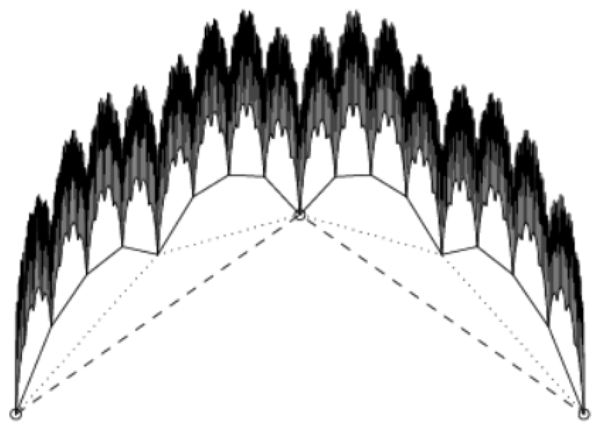
4. Main Theorems of Uniform Convergence of Sequence of Fractal Interpolation Functions and Properties

Theorem 1.

Suppose $\left\{(T{f}_n)(x)\right\}$ is the sequence of fractal interpolation functions generated by affine transformation from Equation (3) to (5), which converges to the attractor $(Tf)(x)$ of $IFS$ defined above, then $\left\{(T{f}_n)(x)\right\}$ uniformly converges to $(Tf)(x)$. Proof On the one hand, since $\left\{(T{f}_n)(x)\right\}$ converges to $(Tf)(x)$, for an arbitrary $\epsilon$ greater than zero, for all $x\in [x_0,x_N]$, so that $\left|(T{f}_n)(x)-(Tf)(x)\right|<\epsilon$ is true.

In the direction of horizontal transformation,

$$\left|a_{n}x+e_n-(a_{m}x+e_m)\right|\le \left|a_n-a\right|\left|x_N\right|+\left|a_m-a\right|\left|x_N\right|+\left|e_n-e\right|+\left|e_m-e\right|<\epsilon$$

In the direction of vertical transformation,

$$\begin{array}{l}\left|(T{f}_n)(x)-(T{f}_m)(x)\right|=\left|c_n{l}_n^{-1}(x)+d_{n}f(l_n^{-1}(x))+f_n-(c_m{l}_m^{-1}(x)+d_{m}f(l_m^{-1}(x))+f_m)\right|\\ \le \left|c_n{l}_n^{-1}(x)-c{l}^{-1}(x)\right|+\left|c_m{l}_m^{-1}(x)-c{l}^{-1}(x)\right|\\ +\left|d_{n}f(l_n^{-1}(x))-df(l^{-1}(x))\right|+\left|d_{m}f(l_m^{-1}(x))-df(l^{-1}(x))\right|\\ +\left|f_n-f\right|+\left|f_m-f\right|<\epsilon \end{array}$$

Therefore, from the Cauchy uniform convergence criterion, the sequence of fractal interpolation functions $\left\{(T{f}_n)(x)\right\}$ uniformly converges to $(Tf)(x)$.

Theorem 2.

Suppose the functions sequence $\left\{(T{f}_n)(x)\right\}$ defined above uniformly converges to $(Tf)(x)$ over the interval $[x_0,x_N]$. If $n$ belongs to positive integer set and there is the following limit formula

$$\underset{x\to x^{\prime }}{\lim }(T{f}_n)(x)=A_n, \mathrm{for} \mathrm{all} x^{\prime }\in [x_0,x_N],$$

then both limit $\underset{n\to \infty }{\lim }{A}_n$ and $\underset{x\to x^{\prime }}{\lim }(T{f}_n)(x)$ exist and they are equal.

Proof. 

At first, it is proved that the limit $\underset{n\to \infty }{\lim }{A}_n$ exists.

In fact, the functions sequence $\left\{(T{f}_n)(x)\right\}$ uniformly converges to its limit function $(Tf)(x)$. That is, for all real numbers $\epsilon >0$, there exists a positive integer $N$ such that, for all integers $n>N$ and an arbitrary positive integer $p$, for all $x\in [x_0,x_N]$, the following formula is true.

$$\begin{array}{l}\left|(T{f}_n)(x)-(T{f}_{n+p})(x)\right|\\ =\left|c_n{l}_n^{-1}(x)+d_{n}f(l_n^{-1}(x))+f_n-(c_{n+p}{l}_{n+p}^{-1}(x)+d_{n+p}f(l_{n+p}^{-1}(x))+f_{n+p})\right|\\ \le \left|c_n{l}_n^{-1}(x)-c_{n+p}{l}_{n+p}^{-1}(x)\right|+\left|c_m{l}_m^{-1}(x)-c{l}^{-1}(x)\right|\\ +\left|d_{n}f(l_n^{-1}(x))-d_{n+p}f(l_{n+p}^{-1}(x))\right|+\left|f_n-f_{n+p}\right|<\epsilon .\end{array}$$

Let $x$ infinitely tend to $x^{\prime }$, there exists the following inequality.

$$\underset{x\to x^{\prime }}{\lim }\left|(T{f}_n)(x)-(T{f}_{n+p})(x)\right|=\left|A_n-A_{n+p}\right|\le \epsilon ,$$

which illustrates the number sequence $\left\{A_n\right\}$ is a convergent number sequence according to the number sequence convergence Cauchy criterion. Let the limit of $\left\{A_n\right\}$ is $B$. The result that the limit $\underset{x\to x^{\prime }}{\lim }(Tf)(x)$ is equal to $B$ can be proved. In fact, since $\left\{(T{f}_n)(x)\right\}$ uniformly converges to its limit function $(Tf)(x)$ and $\underset{n\to \infty }{\lim }{A}_n=B$. In other words, for arbitrary $\epsilon$ greater than zero, there exists a positive integer $N$, so that for all $n>N$, for all $x\in [x_0,x_N]$, the following formula is true.

$$\begin{array}{l}\left|(T{f}_n)(x)-(Tf)(x)\right|\\ =\left|c_n{l}_n^{-1}(x)+d_{n}f(l_n^{-1}(x))+f_n-(c{l}^{-1}(x)+df(l^{-1}(x))+f)\right|<\frac{\epsilon }{3}.\end{array}$$

And $\left|A_n-B\right|<\frac{\epsilon }{3}$.

Especially, choose $n=N+1$,

$$\begin{array}{l}\left|(T{f}_{N+1})(x)-(Tf)(x)\right|\\ =\left|c_{N+1}{l}_{N+1}^{-1}(x)+d_{N+1}f(l_{N+1}^{-1}(x))+f_{N+1}-(c{l}^{-1}(x)+df(l^{-1}(x))+f)\right|\\ =\left|c_{N+1}{l}_{N+1}^{-1}(x)-c{l}^{-1}(x)\right|+\left|d_{N+1}f(l_{N+1}^{-1}(x))-df(l^{-1}(x))\right|+\left|f_{N+1}-f\right|<\frac{\epsilon }{3}.\end{array}$$

And $\left|A_{N+1}-B\right|<\frac{\epsilon }{3}$.

On the other hand, since the following limit formula is true.

$$\underset{x\to x^{\prime }}{\lim }(c_{N+1}{l}_{N+1}^{-1}(x)+d_{N+1}f(l_{N+1}^{-1}(x))+f_{N+1})=A_{N+1}.$$

For the same $\epsilon$ above, there exists a real number $\delta >0$ such that the following inequality holds for all $x$ satisfying $0<\left|x-x_0\right|<\delta$.

$$\left|c_{N+1}{l}_{N+1}^{-1}(x)+d_{N+1}f(l_{N+1}^{-1}(x))+f_{N+1}-A_{N+1}\right|<\frac{\epsilon }{3}.$$

According to the inequality, the following inequality is true.

$$\begin{array}{l}\left|(Tf)(x)-B\right|=\left|c{l}^{-1}(x)+df(l^{-1}(x))+f-B\right|\\ \le |c{l}^{-1}(x)+df(l^{-1}(x))+f-(c_{N+1}{l}_{N+1}^{-1}(x)+d_{N+1}f(l_{N+1}^{-1}(x))+f_{N+1})\\ +(c_{N+1}{l}_{N+1}^{-1}(x)+d_{N+1}f(l_{N+1}^{-1}(x))+f_{N+1})-A_{N+1}+A_{N+1}-B|\\ \le \left|c{l}^{-1}(x)+df(l^{-1}(x))+f-(c_{N+1}{l}_{N+1}^{-1}(x)+d_{N+1}f(l_{N+1}^{-1}(x))+f_{N+1})\right|\\ +\left|c_{N+1}{l}_{N+1}^{-1}(x)+d_{N+1}f(l_{N+1}^{-1}(x))+f_{N+1})-A_{N+1}\right|+\left|A_{N+1}-B\right|\\ <\frac{\epsilon }{3}+\frac{\epsilon }{3}+\frac{\epsilon }{3}<\epsilon ,\end{array}$$

which illustrates when $x\to x^{\prime }$ the limit of the fractal interpolation function $(Tf)(x)$ exists and its limit is equal to $B$. That is, $\underset{x\to x^{\prime }}{\lim }(Tf)(x)=B$. Theorem 2 describes, under the uniform convergence condition of fractal interpolation functions sequence, both the independent variables $x$ and $n$ can exchange limit operations order. That is,

$$\underset{x\to x^{\prime }}{\lim }\underset{n\to \infty }{\lim }(T{f}_n)(x)=\underset{n\to \infty }{\lim }\underset{x\to x^{\prime }}{\lim }(T{f}_n)(x).$$

□

Theorem 3.

The fractal interpolation functions sequence $\left\{(T{f}_n)(x)\right\}$ converges to limit function $(Tf)(x)$ and each of $\left\{(T{f}_n)(x)\right\}$ is continuous over the interval $[x_0,x_N]$, then $(Tf)(x)$ is continuous over the interval $[x_0,x_N]$.

Proof. 

Since each of $\left\{(T{f}_n)(x)\right\}$ is continuous over the interval $[x_0,x_N]$, that is, for all $x\in [x_0,x_N]$, such that the following limit formula is true.

$$\begin{array}{l}\underset{x\to x^{\prime }}{\lim }(T{f}_n)(x)=\underset{x\to x^{\prime }}{\lim }(c_n{l}_n^{-1}(x)+d_{n}f(l_n^{-1}(x))+f_n)\\ =c_n{l}_n^{-1}(x^{\prime })+d_{n}f(l_n^{-1}(x^{\prime }))+f_n=(T{f}_n)(x^{\prime }).\end{array}$$

From Theorem 2,

$$\begin{array}{l}\underset{x\to x^{\prime }}{\lim }(Tf)(x)=\underset{x\to x^{\prime }}{\lim }(c{l}^{-1}(x)+df(l^{-1}(x))+f)\\ =\underset{x\to x^{\prime }}{\lim }\underset{n\to \infty }{\lim }(c_n{l}_n^{-1}(x)+d_{n}f(l_n^{-1}(x))+f_n)\\ =\underset{n\to \infty }{\lim }\underset{x\to x^{\prime }}{\lim }(c_n{l}_n^{-1}(x)+d_{n}f(l_n^{-1}(x))+f_n)\\ =\underset{n\to \infty }{\lim }(c_n{l}_n^{-1}(x^{\prime })+d_{n}f(l_n^{-1}(x^{\prime }))+f_n)\\ =c{l}^{-1}(x^{\prime })+df(l^{-1}(x^{\prime }))+f\\ =(Tf)(x^{\prime }),\end{array}$$

which implies the limit function $(Tf)(x)$ of the fractal interpolation functions sequence $\left\{(T{f}_n)(x)\right\}$ is continuous on the point $x^{\prime }$ and because of the arbitrariness of $x^{\prime }$ on the interval $[x_0,x_N]$, the limit function $(Tf)(x)$ of the fractal interpolation functions sequence is a continuous function over the interval $[x_0,x_N]$. □

Theorem 4.

Let $\left\{(T{f}_n)(x)\right\}$ be the sequence of fractal interpolation functions defined by affine transformation uniformly converges to $(Tf)(x)$ and each of the $\left\{(T{f}_n)(x)\right\}$ is continuous over the interval $[x_0,x_N]$, then the following formula is true.

$$\begin{gathered} {\displaystyle {\int }_{x_0}^{x_N}(}c{l}^{-1}(x)+df(l^{-1}(x))+f)dx \\ =\underset{n\to \infty }{\lim }{\displaystyle {\int }_{x_0}^{x_N}(c_n{l}_n^{-1}(x)+d_{n}f(l_n^{-1}(x))+f_n})dx. \end{gathered}$$

Proof. 

Because $(T{f}_n)(x)=c_n{l}_n^{-1}(x)+d_{n}f(l_n^{-1}(x))+f_n$ uniformly converges to $(Tf)(x)$$=c{l}^{-1}(x)+df(l^{-1}(x))+f$ and each of $(T{f}_n)(x)$ is continuous over the interval $[x_0,x_N]$. From Theorem 2, the sequence of fractal interpolation functions $(T{f}_n)(x)$ and its attractor $(Tf)(x)$ are integral functions over the interval $[x_0,x_N]$.

Since the sequence of fractal interpolation functions $\left\{(T{f}_n)(x)\right\}$ uniformly converges to the function $(Tf)(x)$, then for any given real number $\epsilon >0$, there is a positive integer $N$ so that for all integers $n>N$, the following inequality is true.

$$\begin{array}{l}\left|(T{f}_n)(x)-(Tf)(x)\right|=\left|c_n{l}_n^{-1}(x)+d_{n}f(l_n^{-1}(x))+f_n-(c{l}^{-1}(x)+df(l^{-1}(x))+f)\right|\\ \le \left|c_n{l}_n^{-1}(x)-c{l}^{-1}(x)\right|+\left|d_{n}f(l_n^{-1}(x))-df(l^{-1}(x))\right|+\left|f_n-f\right|<\frac{\epsilon }{x_N-x_0}.\end{array}$$

According to the inequality property of integral, as $n>N$, it follows that

$$\begin{array}{l}\left|{\displaystyle {\int }_{x_0}^{x_N}(T{f}_n})(x)dx-{\displaystyle {\int }_{x_0}^{x_N}(Tf})(x)dx\right|\\ =\left|{\displaystyle {\int }_{x_0}^{x_N}(c_n{l}_n^{-1}(x)+d_{n}f(l_n^{-1}(x))+f_n})dx-{\displaystyle {\int }_{x_0}^{x_N}(}c{l}^{-1}(x)+df(l^{-1}(x))+f)dx\right|\\ \le {\displaystyle {\int }_{x_0}^{x_N}\left|c_n{l}_n^{-1}(x)-c{l}^{-1}(x)+(d_{n}f(l_n^{-1}(x))-df(l^{-1}(x)))+(f_n-f)\right|}\\ \le {\displaystyle {\int }_{x_0}^{x_N}\frac{\epsilon }{x_N-x_0}dx}=\epsilon ,\end{array}$$

That is,

$${\displaystyle {\int }_{x_0}^{x_N}\underset{n\to \infty }{\lim }(c_n{l}_n^{-1}(x)+d_{n}f(l_n^{-1}(x))+f_n})dx=\underset{n\to \infty }{\lim }{\displaystyle {\int }_{x_0}^{x_N}(c_n{l}_n^{-1}(x)+d_{n}f(l_n^{-1}(x))+f_n})dx.$$

□

This completes the proof. Theorem 4 illustrates that both the limit and integral operations can be exchanged under the condition of uniform convergence of the sequence of fractal interpolation functions.

In sum, from Theorem 1 to Theorem 4, the following results have been studied. It is clarified that the fractal interpolation functions sequence is uniformly convergent and the limit function of the sequence of uniform convergence fractal interpolation functions is continuous and integrable over a closed interval.

5. Discussion

It will be very important that uniform convergence of fractal interpolation functions sequence is applied in researching complicated networks, for example, the speed of uniform convergence in the small-world network. Another example, the uniform convergence of the fractal interpolation functions sequence is used to prove the stability of complicated network systems and so on.

References

1. Song, C.M.; Havlin, S.; Makse, H.A. Self-similarity of complex networks. Nature 2005, 433, 392–395. [Google Scholar] [CrossRef] [PubMed] [Green Version]
2. Song, C.M.; Havlin, S.; Makse, H.A. Origins of fractality in the growth of complex networks. Nat. Phys. 2006, 2, 275–281. [Google Scholar] [CrossRef] [Green Version]
3. Bo, L.; Makse, H.A. Topological features of a fractal model for complex networks. In Proceedings of the American Physical Society, APS March Meeting 2012, Boston, MA, USA, 27 February–2 March 2012. [Google Scholar]
4. Barnsley, M.F. Lecture notes on iterated function systems. Proc. Symp. Appl. Math. 1989, 39, 127–144. [Google Scholar]
5. Barnsley, M.F. Fractal functions and interpolation. Constr. Approx. 1986, 2, 303–329. [Google Scholar] [CrossRef]
6. Barnsley, M.F. Fractal interpolation (The sixth chapter). In Fractals Everywhere, 2nd ed.; Elsevier Pte Ltd.: Singapore, 2009; pp. 205–245. [Google Scholar]
7. Massopust, P.R. Fractal surfaces. J. Math. Anal. Appl. 1990, 151, 275–290. [Google Scholar] [CrossRef] [Green Version]
8. Massopust, P.R. Fractal Functions, Fractal Surfaces, and Wavelets, 2nd ed.; Academic Press: Orlando, FA, USA, 1995. [Google Scholar]
9. Gowrisankar, A.; Khalili Golmankhaneh, A.; Serpa, C. Fractal Calculus on Fractal Interpolation Functions. Fractal Fract. 2021, 5, 157. [Google Scholar] [CrossRef]
10. School of Mathematical Sciences, East China Normal University. Thirteenth Chapter Function series. In Mathematical Analysis, 4th ed.; Higher Education Press: Beijing, China, 2010. [Google Scholar]
11. Xu, S.L.; Xue, C.H. Mathematical Analysis; TsingHua University Press: Beijing, China, 2005. [Google Scholar]
Figure 1. A fractal interpolation curve.
Mathematics 10 03834 g001
Figure 2. A fractal interpolation surface.
Mathematics 10 03834 g002
Publisher’s Note: MDPI stays neutral with regard to jurisdictional claims in published maps and institutional affiliations.