Interactions of Logistic Distribution to Credit Valuation Adjustment: A Study on the Associated Expected Exposure and the Conditional Value at Risk

Abstract

In Basel III, the credit valuation adjustment (CVA) was given, and it was discussed that a bank covers mark-to-market losses for expected counterparty risk with a CVA capital charge. The purpose of this study is threefold. Using the logistic distribution, it is shown how the expected exposure can be derived for an interest rate swap. Secondly, the risk measure of VaR is contributed for the CVA under this distribution. Thirdly, generalizations for the CVA VaR and CVA CVaR are given by considering both the credit spread and the expected positive exposure to follow the logistic distributions with different parameters. Finally, several simulations are provided to uphold the theoretical discussions.

1. Introduction

1.1. Credit Valuation Adjustment

Credit valuation adjustment (CVA) is a significant valuation measure in financial engineering that determines how much a financial institute requires adapting a derivative contract value to account for a potential loss of positive exposure when the counterparty is faced with breakdown or default. Technically speaking, CVA is the expected loss of a derivative contract because of the counterparty default.

There is no full theoretical CVA definition. This is normally because regulatory CVA may differ from CVA used for accounting purposes, as well as there being two approaches in computing the CVA capital, i.e., the basic procedure and the standardized procedure [1]. However, we have a CVA formula by considering a continuous stream of cash flows as follows [2]:

$$\mathrm{CVA}(u,T)=(1-R){\int }_u^{T}B(t,T)EE(t,T)DPD(t,T)dt,$$

(1)

where R is the rate of recovery for the counterparty, B is the risk-free discount factor (i.e., $B(t,T)$ represents the time-t value of a risk-free bond with maturity at time T in years), $EE$ is the expected exposure and $DPD$ is the conditional default probability.

In general, we do not know much about the recovery rate. It will depend on the similar factors that influence the probability of default by the counterparty; for more, see [3,4].

Now, by denoting h as the counterparty’s hazard rate (default probability) and V as the expected positive exposure (abbreviated as EPE), and if we assume the involved modeling parameters to be constant over time (and a single cash flow), then the CVA in the continuous-time mode can be given approximately in what follows [5]:

$$\begin{array}{cc}\hfill \mathrm{CVA}& =(1-R){\int }_0^{T}hV{e}^{-(h+r)t}dt,\hfill \\ \hfill & =\frac{h(1-R)V\left(1-e^{-T(h+r)}\right)}{h+r}.\hfill \end{array}$$

(2)

The CVA is essentially based on (i) EPE, (ii) time and (iii) recovery, and partially the hazard rate (h) and the risk-free interest rate (r). To understand the concept of (1) more, we express the counterparty credit risk more in the next subsection. CVA is one of the key pillars of the counterparty credit risk management. In fact, in the regulatory context, the CVA is defined under Basel III as the risk of loss on the over-the-counter (OTC) derivative (financing transaction) due to creditworthiness. Note that the probability measure used here is the pricing measure Q.

Some queries may arise, such as: what causes the fat tail of the exposure? More precisely, in the context of value investing, investors move their money back and forth among trend strategies and value strategies, relying on who has been more successful recently, and, accordingly, fat tails and clustered volatility are produced via temporary increases in destabilizing trend strategies [6]. For further related discussions, one may refer to works [7,8] or chapters of the book [9] by top quantitative analysts Piterbarg, Green, Kjaer, Kenyon and Burgard, who developed the XVA framework over the last decade.

1.2. Counterparty Credit Risk

The concentration of this work is on the credit risk that contains the uncertainty of expected results because of the previous inputs. Counterparty credit risk evaluates the replacement price of a derivative contract to be the default of the counterparty at any time throughout the life term before having the contractual cash flows [10]. Counterparty credit risk depends on several factors, such as exposures, CVA, recovery, collateral, credit ratings, stress scenarios, etc. All of them have some influence on the current state of the economy [11,12,13,14].

Some exposure measures are employed by banks in practice. For instance, the EE profile is mostly employed in pricing counterparty credit risk and in the default risk charges of the Basel regulatory framework. Banks also compute potential future exposures (PFEs) that show a maximum amount of exposure at a high level of confidence, viz., $\alpha =99\%$, at any forthcoming date.

1.3. CVA Value-at-Risk (VaR) and a Variant

By considering $\alpha$ as the pre-determined confidence level, VaR is expressed as follows [15]:

$${\mathrm{VaR}}_{\alpha }\left(X\right):=inf\{z\in \mathbb{R}|F_X\left(z\right)\ge \alpha \},$$

(3)

where $F_X(·)$ is the cumulative distribution function (CDF) and X is a random variable. To discuss the features and shortcomings of (3), we recall that there is sometimes a chance of an adverse market movement that could yield a high loss [16]. The shortcomings of VaR have been discussed in the seminal paper by Artzner et al. in [17] by pointing out that the sub-additivity feature does not hold, and thus loses the coherency.

The CVA VaR according to the Basel III document as a regulatory formula is given by [18] (p. 235):

$$\mathrm{Basel}\mathrm{III}\mathrm{CVA}\mathrm{VaR}=2.33\sqrt{{\eta }_i+\sum _i\frac{3}{4}{w}_i^2{(M_{i}EA{D}_i-M_i{B}_i)}^2},$$

(4)

where

$${\eta }_i={\left(\sum _i\frac{1}{2}{w}_i(M_{i}EA{D}_i-M_i{B}_i)-\sum _i{w}_i{M}_i{B}_i\right)}^2,$$

(5)

where the risk weight for the counterparty i is shown by $w_i$, which is basically a scalar in the range 0.7% to 10% relying on the credit rating of the counterparty, the time horizon is set to 1 year, M stands for the maturity of the exposure/hedge, EAD is the exposure at default (i.e., EE/EPE) and B denotes the notional of the hedge instrument (such as CDS, etc.)

Another risk measure that we used later in this work is the conditional VaR (a.k.a., CVaR), which is a generalization of (3) [19]. The CVaR_α(X) is continuous in terms of $\alpha$. The CVaR can be given as follows:

$${\mathrm{CVaR}}_{\alpha }\left(X\right):=\mathbb{E}\left[X|X\ge {\mathrm{VaR}}_{\alpha }\left(X\right)\right],$$

(6)

where the random variable X is interpreted as a loss variable.

1.4. Motivation

In this work, the logistic distribution was first chosen rather than the well-known normal distribution, which the CVA VaR (4) was built on. The reason is its fatter tail, which is more useful with real observations from the market, which do not follow normal or log-normal distributions [20]. The idea of logistic distribution for obtaining new EE and CVA VaR and CVA CVaR formulas would be fruitful in the counterparty credit risk.

Some remarks are in order:

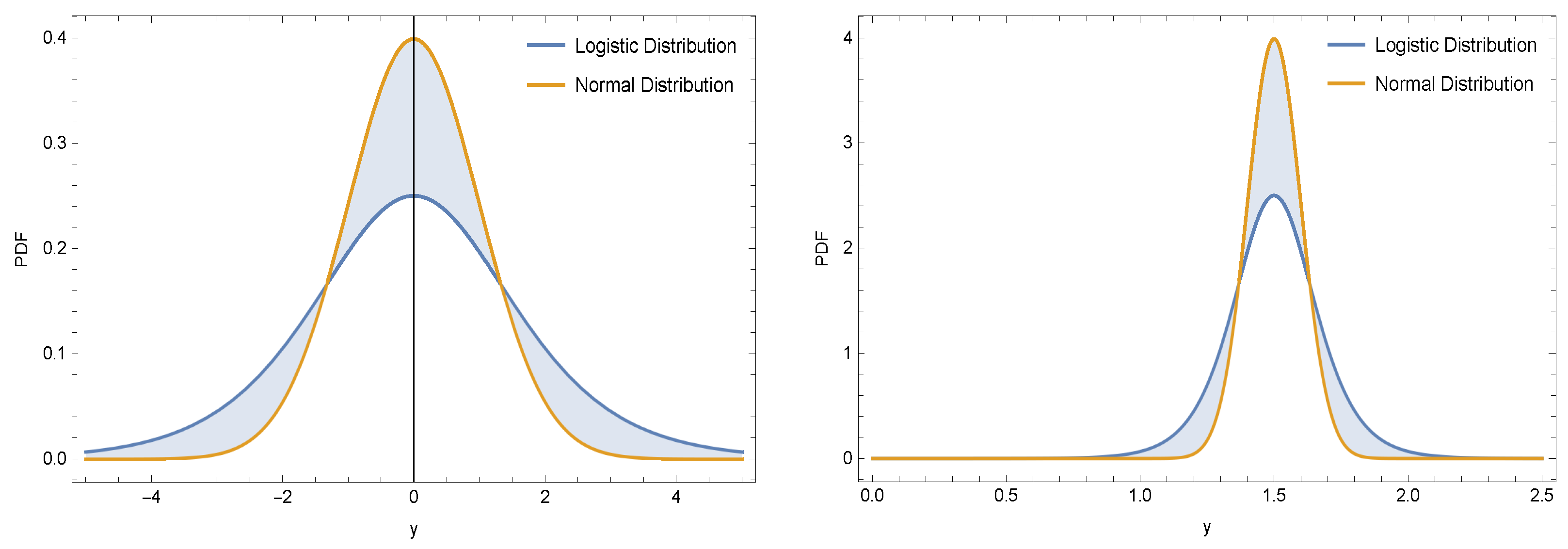
• As pointed out in [21], credit spread levels and changes provide signs of the characteristic fat-tailed behavior and, in both cases, recommend that both series are away from a distribution of the normal. This justifies why we chose the fatter tail logistic distribution in this work in contrast to the normal distribution.
• The logistic model has also recently been applied in the work [22] in another context and showed promising results.
• It is pointed out that, in Table 1 of [23], some empirical evidence for the use of a logistic distribution for modeling the distribution of a risk variable is provided.
• Note that experiencing all of the non-Gaussian distributions in modeling stock data [24] is not the major aim here since it is not feasible. As a matter of fact, our strategy is to adopt a fat-tailed distribution, namely, logistic distribution, that is good enough to accommodate the features of financial data with respect to computing the CVA VaR and CVA CVaR in higher dimensions.

To incorporate the dependence among the factors existing in a CVA formulation, in terms of a mathematical point of view, we consider not only the spread rate but also the EPE to not be constant any more and to follow logistic distributions. However, such a dependence can be followed by other approaches, such as defining a copula function on the spread rate and the EPE. For precise definitions of EE, PFE, EPE, etc., readers can refer to [25] (Chapter 2).

1.5. Problems to Be Solved and Novelty

An interest rate swap’s (IRS’s) effective description is a derivative contract, agreed between two counterparties, that determines the nature of an exchange of payments benchmarked against an interest rate index. Accordingly:

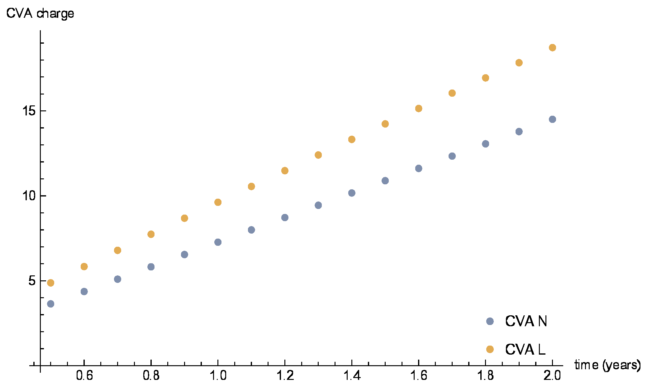
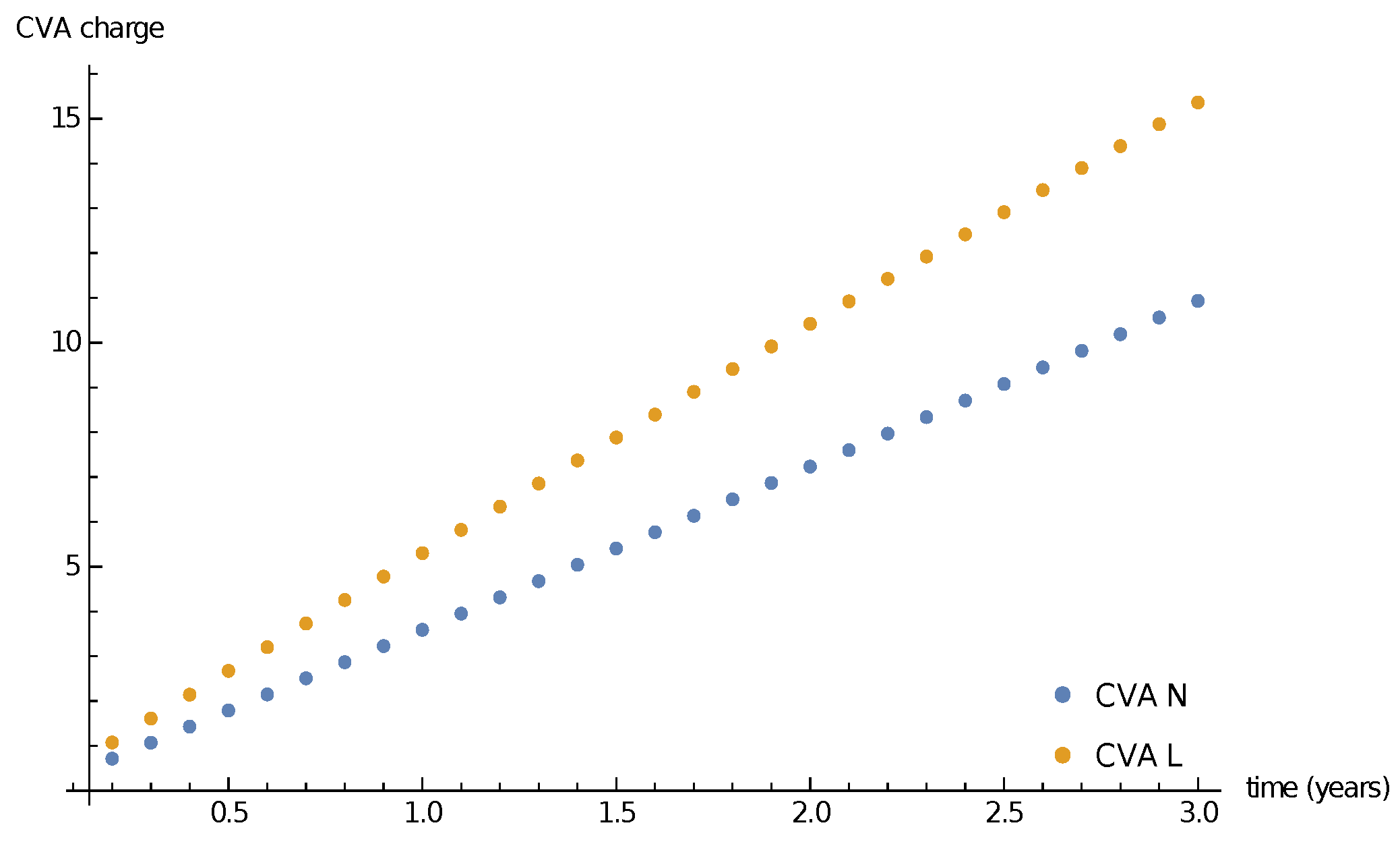
• Here, we first focused on IRS CVA and improved the existing EEs formulas given for IRS CVA using the logistic distribution. The existing relations are based on the normal distribution. In fact, here, the novelty is that we explored the model distribution for the exposure based on a proxy for the swap duration and the logistic distribution.
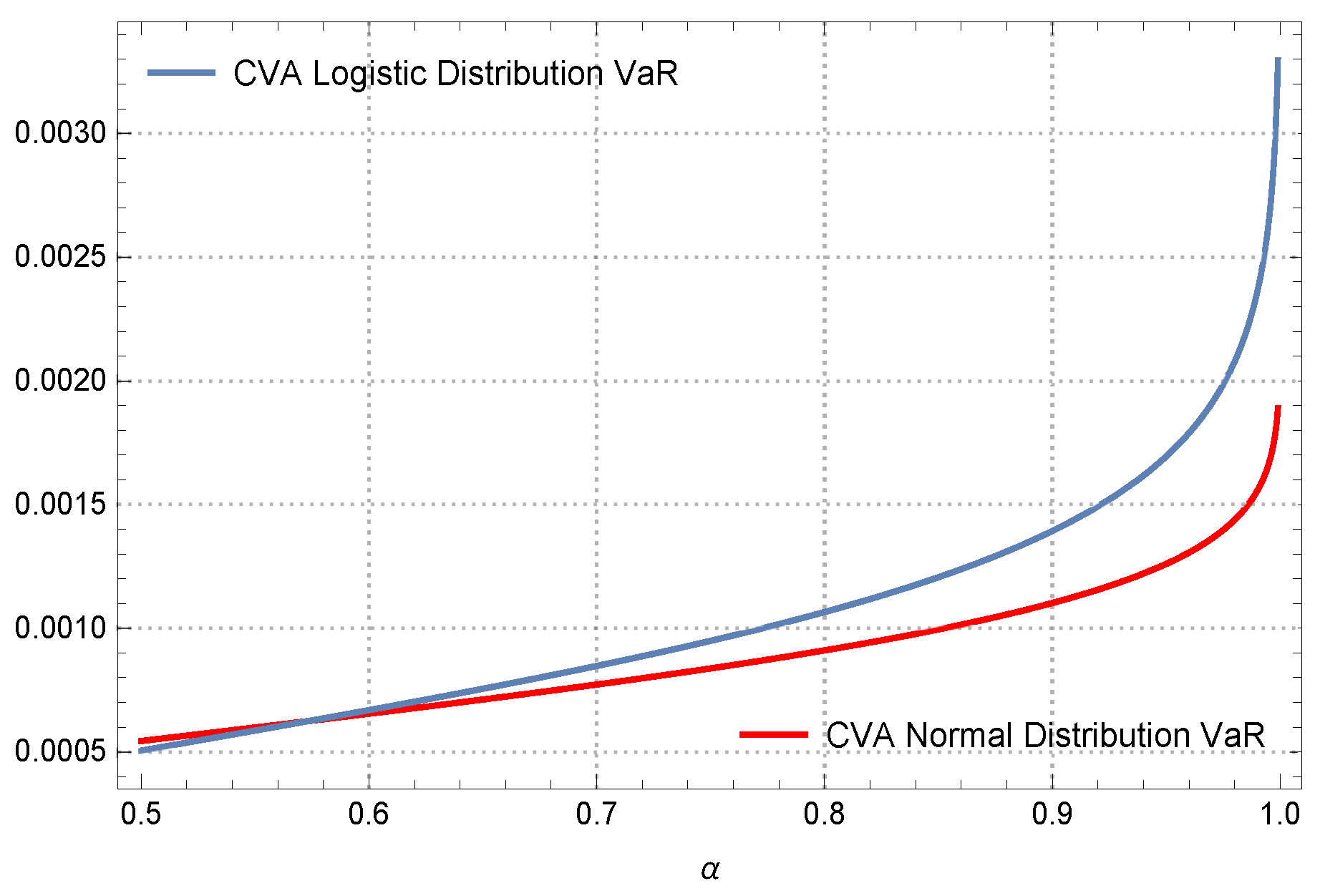
• Next, we employed the logistic distribution to propose a new formulation for CVA VaR. In fact, the existing CVA VaR formulation is based on the normal distribution and, here, we assumed that the CDS spread follows a logistic distribution and obtained a new formulation that is more consistent with real financial data having fatter tails.
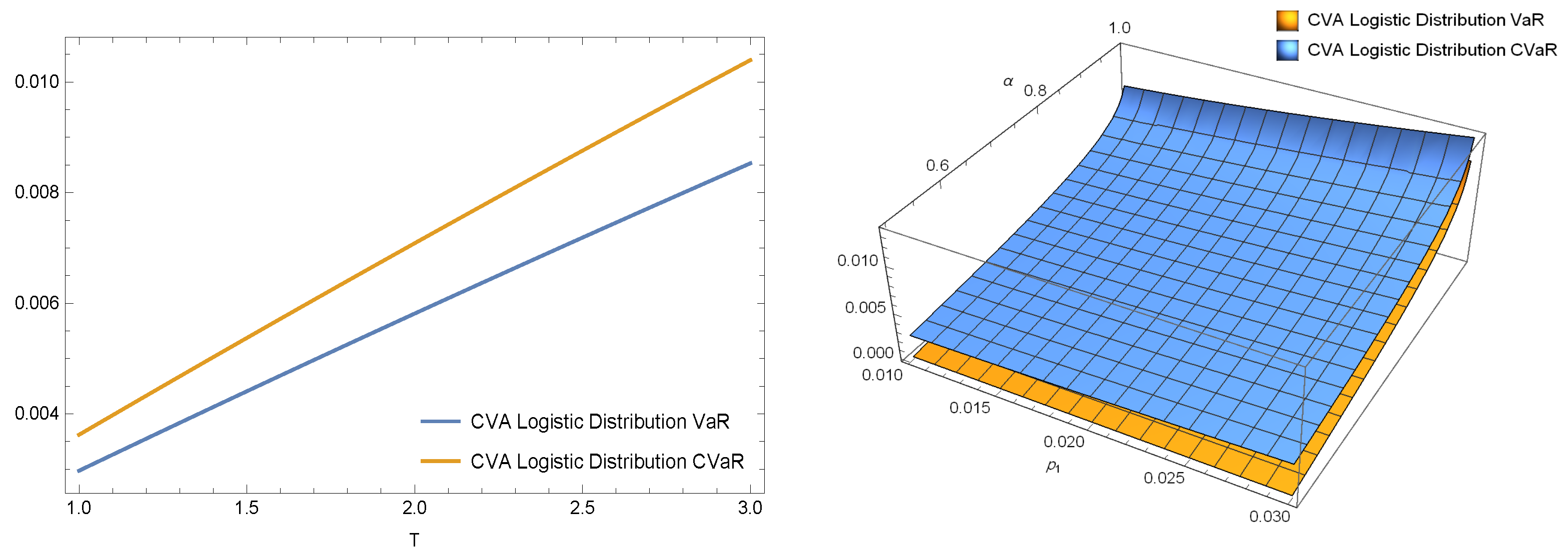
• The final important factor that has been addressed in this piece of work is to assume that not only the credit spread but also the EPE follow logistic distributions having different parameters. This novelty of the work extends the computation of CVA VaR and CVaR in higher dimensions.

To discuss further, an indication of the added value of the current research in the actual literature is that an extension for the CVA logistic VaR and CVA logistic CVaR are contributed by considering both the credit spread and the EPE to follow the logistic distributions with different parameters.

1.6. Organization

The remaining sections are structured as follows. Since one focus of this article is on IRS CVA, in Section 2, the new EEs for this heavy-tail distribution were constructed. Laplace distribution has wider tails than the normal distribution, so it is more applicable with the financial data and furnishes a further understanding of the likelihood of extreme events; for more details, refer to [26]. Then, Section 3 is devoted to the derivation of new analytic formulations for the CVA VaR and CVA CVaR under the logistic distribution. Next, Section 4 discusses the applicability and usefulness of the contributed formulas in practice. Several comparisons are made, along with numerical simulations. At last, a summary of the work, along with some comments for forthcoming works, are provided in Section 5.

2. New EE Formulas

2.1. Logistic Distribution

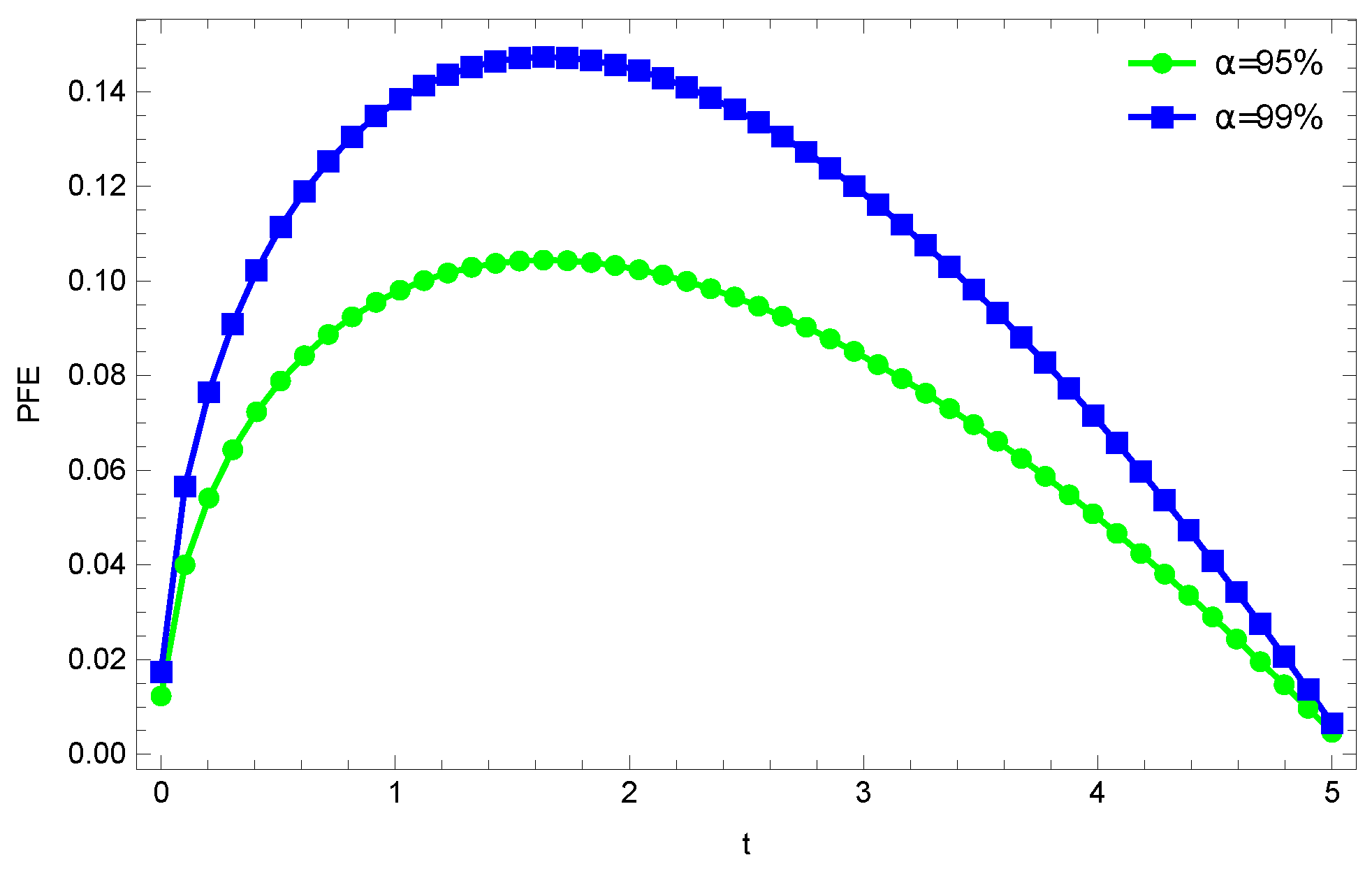
The logistic distribution on the set of real numbers $\mathbb{R}$ gives a statistical continuous distribution under the two constants $\mu$ and $\sigma$ as its mean and scale parameter, respectively. The PDF of this has a single peak, though its overall curve is obtained via the parameters of $\mu$ and $\sigma$.

Now, assume that Y is a stochastic variable and is distributed by $Y\sim \mathrm{Logistic}(\mu ,\sigma )$. The CDF for this distribution could be attained as [26]: $F\left(y\right)=\frac{1}{e^{-\frac{y-\mu }{\sigma }}+1},$ whereas its PDF is given by: $f\left(y\right)=\frac{e^{-\frac{y-\mu }{\sigma }}}{\sigma {\left(e^{-\frac{y-\mu }{\sigma }}+1\right)}^2}$.

To show the characteristics of this distribution, we show

Table 1. Features for the two compared continuous distributions.

Name	Mean	Variance	Median	Skewness	Kurtosis	q-Quantile
Normal	$\mu$	${\sigma }^2$	$\mu$	0	3	$\mu -\sqrt{2}\sigma {\mathrm{erfc}}^{-1}\left(2q\right)$, $0\le q\le 1$
Logistic	$\mu$	$\frac{{\pi }^2{\sigma }^2}{3}$	$\mu$	0	$\frac{21}{5}$	$\mu -\sigma log\left(\frac{1}{q}-1\right)$, $0<q<1$

, which provides different features of the logistic distribution in comparison to the normal distribution. In Table 1, we have $\mathrm{erfc}\left(z\right)=1-\frac{2}{\sqrt{\pi }}{\int }_0^z{e}^{-t^2}dt$. Throughout the work, $log(·)$ stands for the natural logarithm. In order to compare the PDFs of the normal and logistic distributions, they are plotted in Figure 1. The major difference between the logistic and the normal distributions lies in the tails and in the behavior of the failure rate function.

2.2. PFE

In order to calculate the CVA charge for the IRS, we proceeded as follows. A popular model for interest rates (IRs), which was constructed by a sole source of market risk, is the stationary Ornstein–Uhlenbeck (OU) SDE process with long-term mean $\mu$, volatility $\sigma$ (non-zero real number), speed of adjustment $\theta$ and positive real number $x_0$ as the initial condition as follows [27] (chapter 7.3.3):

$$dx\left(t\right)=\theta (\mu -x(t\left)\right)dt+\sigma dw\left(t\right),$$

(7)

where $w\left(t\right)$ is a standard Wiener process and $x\left(t\right)$ is the OU process. Here, $\mu$ and $\theta$ are non-zero real numbers of the same sign.

Now, in order to compute the exposure based on (7), we obtain the model distribution for the exposure in the form [28]:

$$(T-t)\left(x\right(t)-s),$$

(8)

where s is the deal swap rate and $T-t$ is the proxy for the swap duration.

Thus, we have a transformed distribution (each may have different distributions under several assumptions) on (8) where $x\left(t\right)$ is an OU process, $T>t$ and $x>0$. This can be deduced as

$$(T-t)(x\left(t\right)-s)\sim \mathrm{Normal}\left[{ϵ}_1,{ϵ}_2\right],$$

(9)

where

$$\begin{array}{cc}\hfill {ϵ}_1& =e^{\theta (-t)}(t-T)(\mu +(s-\mu )e^{\theta t}-x_0),\hfill \\ \hfill {ϵ}_2& =\frac{\sigma \sqrt{\frac{1-e^{-2\theta t}}{\theta }}(T-t)}{\sqrt{2}}.\hfill \end{array}$$

(10)

Now, the maximum EP under the confidence level $\alpha$ is obtained, i.e., how far can exposure go under a given level of confidence. Using the inverse CDF, we find the PFE as follows ($T>t$:)

$$\mathrm{PFE}=e^{\theta (-t)}(t-T)\left(\sigma {\mathrm{erfc}}^{-1}\left(2\alpha \right)e^{\theta t}\sqrt{\frac{1-e^{-2\theta t}}{\theta }}+\mu +(s-\mu )e^{\theta t}-x_0\right).$$

(11)

Here, the exposure as a function of the OU model is normally distributed.

To have a better picture, this is plotted in Figure 2 for various values of $\alpha$ on the time horizon $t\in [0,5]$. As a matter of fact, Figure 2 is the profile of a 5Y ATM swap with a 3.5% spread rate s in (11) with 1.5% swap volatility, as well as $\mu =0.04$, $\theta =0.03$, $x_0=0.035$.

2.3. Derivation of New EE Relations

While potential exposure is a good measure to see where the exposure can go, in most cases, we are interested in the average exposure over the time of transaction. This is exactly what carries out the EE.

To calculate the EE, we here assume further that $x\left(t\right)$ can follow the logistic distribution, unlike the normal distribution (9). In fact, we consider that the normal distribution can be approximated by a logistic distribution having fatter tails [29]. It is well known that the logistic and normal distributions are quite similar, since the respective distributions determined by a location and a scale parameter are both bell-shaped. Accordingly, we consider

$$x\sim \mathrm{Logistic}[\mathrm{a},\mathrm{b}],$$

(12)

and then take the expectation with respect to logistic distribution (12). Since the exposure is directional, we compute separate measures from (8) for both the payer and receiver swap, respectively, as follows:

$$\begin{array}{ccc}\hfill \mathbb{E}\left[(T-t){\Omega }_1,\right.& \left.x\sim \mathrm{Logistic}[\mathrm{a},\mathrm{b}]\right]\hfill & \\ \hfill & ={\int }_{-\infty }^{+\infty }\left((T-t){\Omega }_1\right)\frac{e^{-\frac{x-\mu }{\sigma }}}{\sigma {\left(e^{-\frac{x-\mu }{\sigma }}+1\right)}^2}dx\hfill & \\ \hfill & =(t-T)\left(s-blog\left(e^{a/b}+e^{s/b}\right)\right),\hfill \end{array}$$

(13)

where

$${\Omega }_1=\left\{\begin{array}{cc}x-s\hfill & x>s,\hfill \\ 0\hfill & \mathrm{otherwise}.\hfill \end{array}\right.$$

Now, we have:

$$\begin{array}{ccc}\hfill \mathbb{E}\left[(T-t){\Omega }_2,\right.& \left.x\sim \mathrm{Logistic}[\mathrm{a},\mathrm{b}]\right]\hfill & \\ \hfill & ={\int }_{-\infty }^{+\infty }\left((T-t){\Omega }_2\right)\frac{e^{-\frac{x-\mu }{\sigma }}}{\sigma {\left(e^{-\frac{x-\mu }{\sigma }}+1\right)}^2}dx\hfill & \\ \hfill & =(t-T)\left(a-blog\left(e^{a/b}+e^{s/b}\right)\right),\hfill \end{array}$$

(14)

where

$${\Omega }_2=\left\{\begin{array}{cc}s-x\hfill & s>x,\hfill \\ 0\hfill & \mathrm{otherwise}.\hfill \end{array}\right.$$

When computing the CVA, the exposure is non-negative; see, e.g., expression (1). Finally to obtain the EE explicitly, we first obtain the following mean and volatility parameters from the OU model (7) (using a similar methodology as in [30] by taking advantage of Itô lemma and the crucial properties of Itô integral.)

To calculate the mean and variance of the linear SDE (7), we proceed as follows. The solution of (7) reads:

$$x\left(t\right)=\mu +(x_0-\mu )e^{-\theta t}+\sigma {\int }_0^t{e}^{-\theta (t-s)}dw\left(s\right).$$

(15)

Hence, the expectation of $x\left(t\right)$ can be written as follows:

$$\begin{array}{cc}\hfill \mathbb{E}\left[x\right(t\left)\right]& =\mathbb{E}\left[\mu +(x_0-\mu )e^{-\theta t}+\sigma {\int }_0^t{e}^{-\theta (t-s)}dw\left(s\right)\right],\hfill \\ \hfill & =\mu +(x_0-\mu )e^{-\theta t}+\sigma \mathbb{E}\left[{\int }_0^t{e}^{-\theta (t-s)}dw\left(s\right)\right],\hfill \\ \hfill & =\mu +(x_0-\mu )e^{-\theta t}.\hfill \end{array}$$

(16)

Similarly, for the variance, we have

$$\begin{array}{cc}\hfill \mathrm{Var}\left[x\right(t\left)\right]& =\mathbb{E}\left[x{\left(t\right)}^2\right]-\mathbb{E}{\left[x\left(t\right)\right]}^2,\hfill \\ \hfill & =\mathbb{E}\left[{\left(\mu +(x_0-\mu )e^{-\theta t}+\sigma {\int }_0^t{e}^{-\theta (t-s)}dw\left(s\right)\right)}^2\right]-{(\mu +(x_0-\mu )e^{-\theta t})}^2,\hfill \\ \hfill & ={(\mu +(x_0-\mu )e^{-\theta t})}^2+2\sigma {(\mu +(x_0-\mu )e^{-\theta t})}^2\mathbb{E}\left[{\int }_0^t{e}^{-\theta (t-s)}dw\left(s\right)\right]\hfill \\ \hfill & +{\sigma }^2\mathbb{E}\left[{\left({\int }_0^t{e}^{-\theta (t-s)}dw\left(s\right)\right)}^2\right]-{(\mu +(x_0-\mu )e^{-\theta t})}^2,\hfill \\ \hfill & ={\sigma }^2\mathbb{E}\left[{\int }_0^t{e}^{-2\theta (t-s)}d\left(s\right)\right],\hfill \\ \hfill & ={\sigma }^2{\int }_0^t{e}^{-2\theta (t-s)}d\left(s\right),\hfill \\ \hfill & =\frac{{\sigma }^2}{2\theta }(1-e^{-2\theta t}),\hfill \end{array}$$

(17)

where the Itô isometry has been used for simplifications. Here, we used the assumptions that $\mu$ and $\theta$ are constant.

Now, the EE for the payer can be proposed from (13) by substituting a and b from (16) and (17) as follows:

$${\mathrm{EE}}_p=\frac{1}{2}(t-T)\left(2s-\sigma \sqrt{\frac{2-2e^{-2\theta t}}{\theta }}log\left(\psi \right)\right),$$

(18)

where

$$\psi =e^{\left(\frac{\sqrt{2}\left(\mu +e^{\theta (-t)}(x_0-\mu )\right)}{\sigma \sqrt{\frac{1-e^{-2\theta t}}{\theta }}}\right)}+e^{\frac{\sqrt{2}s}{\sigma \sqrt{\frac{1-e^{-2\theta t}}{\theta }}}}.$$

(19)

Similarly, the EE for the receiver can be deduced as follows:

$${\mathrm{EE}}_r=(t-T)\left(-\frac{\sigma \sqrt{\frac{1-e^{-2\theta t}}{\theta }}log\left(\psi \right)}{\sqrt{2}}+\mu +e^{\theta (-t)}(x_0-\mu )\right).$$

(20)

The relations (18) and (20) are further illustrated computationally in Section 4.

3. Novel Risk Measure Formulas for CVA

3.1. CVA VaR under the Logistic Distribution

Here, it is recalled that the author in [5] proposed the VaR formulation under the logistic distribution ($Y\sim \mathrm{Logistic}(\mu ,\sigma )$) as follows:

$${\mathrm{VaR}}_{\alpha }\left(Y\right)=\mu -\sigma log\left(\frac{1}{\alpha }-1\right),$$

(21)

which would be used later in this section.

Let us now choose

$$h(1-R)=s,$$

(22)

in (2) to yield:

$$\mathrm{CVA}=\frac{sV\left(1-e^{-T(h+r)}\right)}{h+r}.$$

(23)

The relation (23) shows that the CVA is a product of three factors: (i) risky duration, (ii) EPE and (iii) CDS spread. Since the duration impact is rather limited, we follow the Basel logic and conclude that CVA changes due to the counterparty creditworthiness deterioration [31], i.e., the widening of the credit spread s. This takes us to an elegant formula that we can derive under the logistic distribution in the following theorem.

Here, s is in the $L^{\mathfrak{p}}$ spaces, which are function spaces defined by a natural extension of the $\mathfrak{p}$-norm for finite-dimensional vector spaces.

Theorem 1.

Let the credit spread $s\in L^{\mathfrak{p}}$ be a random variable presenting a continuous distribution under the $\mathrm{Logistic}(p,q)$; then, the CVA VaR measure is provided in the following closed form:

$$\mathit{CVA}\mathit{VaR}=\frac{V{e}^{T(-(h+r\left)\right)}\left(e^{T(h+r)}-1\right)\left(p-qlog\left(\frac{1}{\alpha }-1\right)\right)}{h+r}.$$

Proof. 

Having s be distributed by the logistic distribution, we obtain the following transformed distribution:

$$\frac{sV\left(1-e^{-T(h+r)}\right)}{h+r}\sim \mathrm{Logistic}\left[\frac{pV\left(1-e^{-T(h+r)}\right)}{h+r},\frac{qV\left(1-e^{-T(h+r)}\right)}{h+r}\right].$$

(24)

Note that, here, p and q are the credit spread mean and its volatility, respectively. Now, by employing (24) in (3) and (21), we have

$$\begin{array}{ccc}\hfill \mathrm{CVA}\mathrm{VaR}& =min\{z\in \mathbb{R}|F_Y\left(z\right)\ge \alpha \},\hfill & \hfill 0<\alpha <1,\\ \hfill & =\frac{V{e}^{T(-(h+r\left)\right)}\left(e^{T(h+r)}-1\right)\left(p-qlog\left(\frac{1}{\alpha }-1\right)\right)}{h+r},\hfill & \hfill 0<\alpha <1.\end{array}$$

(25)

The proof is complete. □

3.2. Extension to Higher Dependency Based on the Logistic Distribution

We can extend the CVA model (24) further to incorporate an additional factor—say, (i) EPE—and (ii) bring the dependency pattern into the model.

Let us consider (23) to be influenced under two continuous distributions on the most important elements of the credit spread and EPE as follows:

$$\zeta =\frac{sV\left(1-e^{-T(h+r)}\right)}{h+r},s\sim \mathrm{Logistic}\left[p_1,q_1\right],V\sim \mathrm{Logistic}\left[p_2,q_2\right].$$

(26)

Here, we do not assume that the product of two logistically distributed variables is logistically distributed, since this is not true in general and a mixture distribution must be obtained. In fact, we consider that both s and V come from the logistic distribution when they are not constant. In such a case, the CVA VaR and CVA CVaR are best addressed in the following theorem.

Theorem 2.

Having the conditions of Theorem 1, the CVA VaR and CVA CVaR measures employing the logistic distribution are derived in closed forms as follows:

$$\mathrm{CVA}\mathrm{VaR}=-\frac{1}{3}\pi log\left(\frac{1}{\alpha }-1\right)\vartheta ,$$

(27)

where

$$\vartheta =\sqrt{\frac{\left(3p_2^2{q}_1^2+q_2^2\left(3p_1^2+{\pi }^2{q}_1^2\right)\right)e^{-2T(h+r)}{\left(e^{T(h+r)}-1\right)}^2}{{(h+r)}^2}}.$$

(28)

In addition,

$$\mathit{CVA}\mathit{CVaR}=-\frac{\pi \vartheta \left(log\left(\frac{1}{1-\alpha }\right)+\alpha \left(log(1-\alpha )+log\left(\frac{1}{\alpha }\right)\right)\right)}{3(\alpha -1)}.$$

(29)

Proof. 

By taking into account that $h>0$, $T>0$ and $r>0$, and since a direct VaR formula does not exist, we first compute the mean and variance of the transformed distribution (26) as follows:

$$\begin{array}{cc}\hfill \mathbb{E}\left[\zeta \right]& =\frac{p_1{p}_2{e}^{T(-(h+r\left)\right)}\left(e^{T(h+r)}-1\right)}{h+r}.\hfill \end{array}$$

(30)

$$\begin{array}{cc}\hfill \mathrm{Var}\left[\zeta \right]& =\frac{{\pi }^2\left(3p_2^2{q}_1^2+q_2^2\left(3p_1^2+{\pi }^2{q}_1^2\right)\right)e^{-2T(h+r)}{\left(e^{T(h+r)}-1\right)}^2}{9{(h+r)}^2}.\hfill \end{array}$$

(31)

Now, by replacing the standard deviation from (31) into the relation (21), we obtain the CVA VaR under the logistic distribution for the two-dimensional case as comes next (27). In a similar manner, by employing (6) and the following CVaR formulation proposed by Hlivka in [5] for the logistic distribution ($Y\sim \mathrm{Logistic}(\mu ,\sigma )$):

$${\mathrm{CVaR}}_{\alpha }\left(Y\right)=\frac{\alpha \mu -\sigma log\left(\frac{1}{1-\alpha }\right)-\alpha \sigma log(1-\alpha )-\alpha \sigma log\left(\frac{1}{\alpha }\right)-\mu }{\alpha -1},$$

(32)

we can construct the CVA CVaR formulation under the bi-logistic distribution as (29). The proof has now ended. □

4. Applications

The aim of this section is to check and uphold the contributed EE formulations and the CVA risk measures of Section 2 and Section 3. The simulations here were performed employing Mathematica 12.0 [32] on a laptop with Windows 10 Home and a Core i7-9750H CPU having 16GB of RAM along with SSD memory.

No special data are used in this section and the set of parameters were taken from the literature, as cited accordingly.

The most famous kind of swaps includes IRS, where one side exchanges a floating rate loan for a fixed rate loan. The net present value of the fixed cash flows of an IRS is then named as the fixed leg and the expected net present value of the floating cash flows is named by the floating leg. If the fixed leg is paid and the floating leg is received, one calls the agreement a payer IRS, whereas if the floating leg is paid and the fixed leg is received, one can name it a receiver IRS or receiver swap.

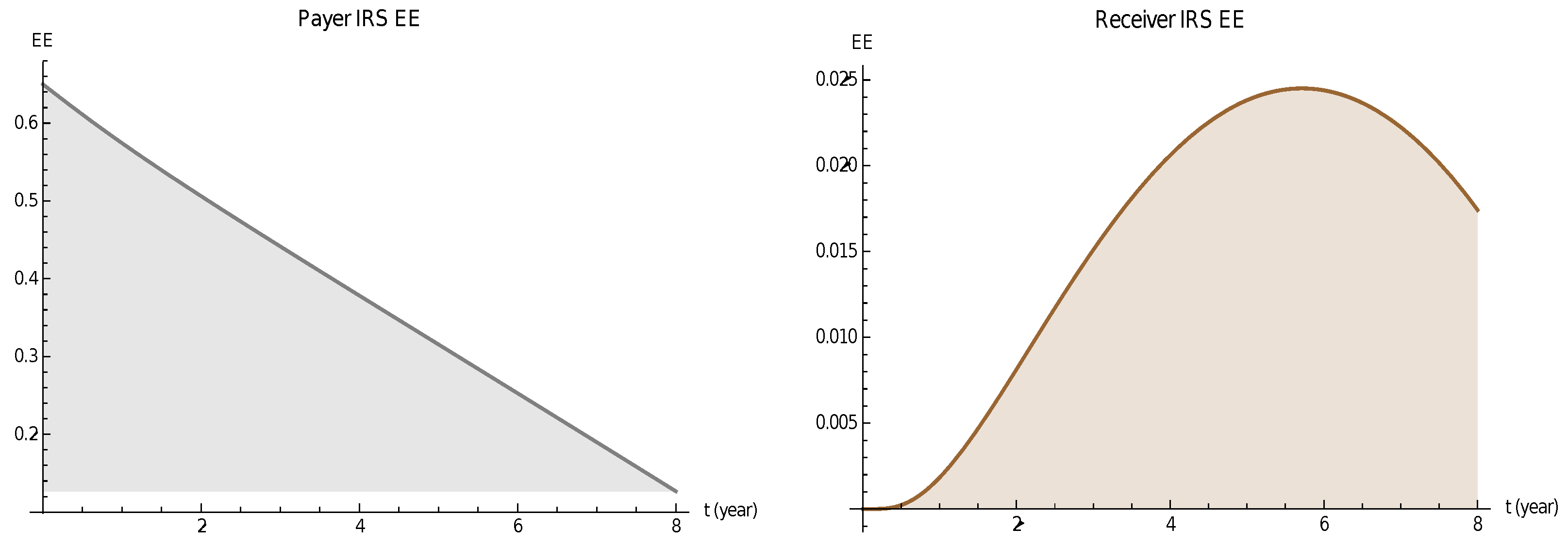
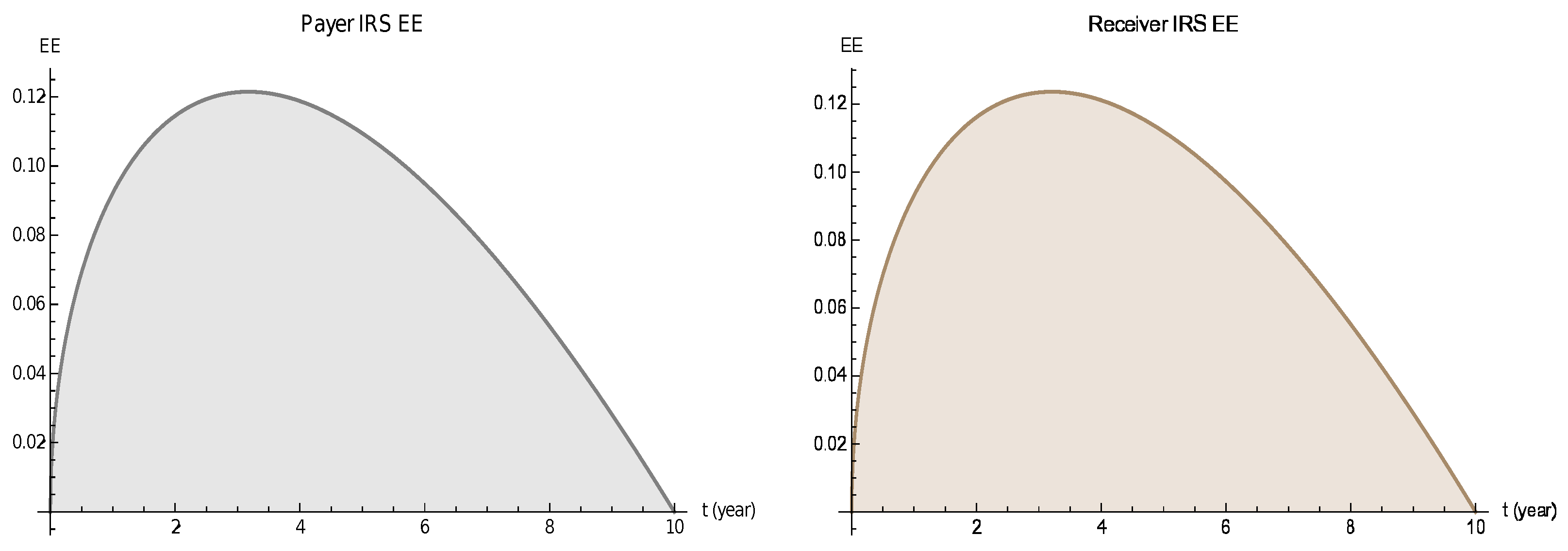
4.1. EEs for the Payer and Receiver Swap

The computational EEs for the payer and receiver swap are given in Figure 3 and Figure 4 based on (18) and (20). Here, the set of parameters are [28]:

$$s=0.035,T=max\left\{t\right\}\mathrm{years},\mu =0.03,\theta =0.02,\sigma =0.015.$$

(33)

As we can see, the EE has a much lower quantity if compared to the PFE as expected for various values of time and the initial conditions.

To theoretically show that CVA L>CVA N, we must investigate that the following holds true:

$$\frac{V{e}^{T(-(h+r\left)\right)}\left(e^{T(h+r)}-1\right)\left(p-qlog\left(\frac{1}{\alpha }-1\right)\right)}{h+r}>\frac{pV\left(e^{T(h-r)}-1\right)}{h-r}-\sqrt{2}qV{\mathrm{erfc}}^{-1}\left(2\alpha \right)\Delta ,$$

(34)

where $\Delta =\frac{e^{T(h-r)}-1}{h-r}$. Note that $\Delta$ is always positive regardless of the choice of $h>r$ or $r>h$. This depends on the choice of the parameters. However, as long as the parameters are positive and chosen properly, then it holds. To formally pursue this, we might go on (approximately) by writing the Taylor expansion of the left and right sides of (34) as follows:

$$\frac{V{e}^{T(-(h+r\left)\right)}\left(e^{T(h+r)}-1\right)\left(p-qlog\left(\frac{1}{\alpha }-1\right)\right)}{h+r}=TV\left(p-qlog\left(\frac{1}{\alpha }-1\right)\right)+O\left(T^2\right),$$

(35)

and

$$\frac{pV\left(e^{T(h-r)}-1\right)}{h-r}-\sqrt{2}qV{\mathrm{erfc}}^{-1}\left(2\alpha \right)\Delta =pTV-\sqrt{2}qVT{\mathrm{erfc}}^{-1}\left(2\alpha \right)+O\left(T^2\right),$$

(36)

which is the Taylor expansion up to the first order on T, h and r. On the other hand, as long as $p,q,V>0$, $\alpha >1/2$, by using (35) and (36), we have ${\mathrm{erfc}}^{-1}\left(2\alpha \right)<0$ and

$$-qTVlog\left(\frac{1}{\alpha }-1\right)>-\sqrt{2}qTV{\mathrm{erfc}}^{-1}\left(2\alpha \right).$$

(37)

Then, we obtain

$$log\left(\frac{1}{\alpha }-1\right)<\sqrt{2}{\mathrm{erfc}}^{-1}\left(2\alpha \right).$$

(38)

Note that this gives a condition on the choice of $\alpha$ to have (34). However, as long as $\alpha \gg 1/2$, then it would be valid. From the point of view of the real application of the CVA L indicator, or other similar indicators, $\alpha$ must be close to 1 and, in almost all cases, it is considered to be higher than 90% to clearly give a proper sight of the risk involved in the financial problem. It is also noted that this does not contradict the results in Figure 5 around $\alpha =1/2$, since, first of all, (38) is obtained based on the first order Taylor expansion, which is an approximation procedure, and, second, it reveals that, as long as we get close to $\alpha =1/2$ (although this does not happen in practice), and only theoretically, more data can be covered by the normal PDF rather than the logistic PDF, which is a confirmation of Figure 1, and, once again, says that the fatter tail helps us in risk management when $\alpha \gg 1/2$.

4.2. Results for 1D CVA VaR and Advantages over the Existing Solver

To check the validity of (25), the CVA charges are obtained via (25) and compared to the values of CVA normal VaR (CVA N) and CVA logistic VaR (CVA L) in

Table 2. CVA charges in comparisons to the CVA N and CVA L.

T	2.0	2.1	2.2	2.3	2.4	2.5	2.6	2.7	2.8	2.9	3.0
CVA charge	3.44	3.60	3.77	3.93	4.09	4.25	4.41	4.57	4.73	4.89	5.05
CVA N, $\alpha =80\%$	6.05	6.35	6.66	6.96	7.27	7.57	7.88	8.187	8.49	8.79	9.10
CVA L, $\alpha =80\%$	7.26	7.60	7.95	8.29	8.63	8.97	9.31	9.6517	9.98	10.3211	10.65
CVA N, $\alpha =90\%$	7.32	7.69	8.06	8.43	8.80	9.17	9.54	9.90	10.27	10.64	11.01
CVA L, $\alpha =90\%$	9.49	9.94	10.39	10.84	11.29	11.73	12.18	12.62	13.05	13.49	13.93
CVA N, $\alpha =95\%$	8.37	8.80	9.22	9.64	10.06	10.48	10.90	11.33	11.75	12.17	12.60
CVA L, $\alpha =95\%$	11.55	12.10	12.65	13.19	13.74	14.28	14.82	15.35	15.88	16.42	16.95
CVA N, $\alpha =99\%$	10.35	10.87	11.39	11.91	12.43	12.95	13.47	13.99	14.52	15.04	15.56
CVA L, $\alpha =99\%$	16.09	16.86	17.63	18.39	19.14	19.90	20.65	21.39	22.14	22.88	23.62

. The considered parameters here are:

$$r=0.02,h=0.015/0.6=0.025,V=0.012,R=0.4,p=0.015,q=0.012.$$

(39)

Note that the default probability h is equal to the CDS value s over $1-R$.

Since most financial data are characterized by leptokurtosis (fat-tails), the usefulness of the logistic distribution can be confirmed from Table 2. Results are given in bp (basis points, e.g., one basis point is equal to 1/100th of 1%, or 0.01% or 0.0001) and show that, for confidence levels of more than 50%, the CVA L gives a better hedge rather than CVA N. The CVA L values for the 99% are higher than the CVA N measure, which is what we expected.

Remark 1.

From Table 2, the CVA VaR values from the normal and logistic distributions at the 99% confidence level may be around three to four times higher than the respective CVA charges. In addition, from Table 2, the CVA VaR values from the logistic distribution are less than double of the respective CVA VaR values from the normal distribution.

Finally, the shape of the CVA logistic VaR is plotted in Figure 5, which is very similar to the market risk VaR and is compared to CVA L.

Now, three more case studies, in order to confirm the superiority of the use of logistic distribution instead of normal distribution, are given based on

$$\mathrm{Case}\mathrm{A}:r=0.03,h=0.015/0.6=0.025,V=0.02,p=0.02,q=0.01,\alpha =0.95.$$

$$\mathrm{Case}\mathrm{B}:r=0.01,h=0.015/0.6=0.025,V=0.01,p=0.01,q=0.02,\alpha =0.90.$$

$$\mathrm{Case}\mathrm{C}:r=0.05,h=0.015/0.6=0.025,V=0.05,p=0.02,q=0.02,\alpha =0.99.$$

The results are reported in Figure 6, Figure 7, Figure 8 and Figure 9, re-confirming the superiority.

4.3. Results for 2D CVA VaR

The sets of parameters in Figure 6 (left and right) are as follows, respectively:

$$r=0.02,h=0.015/0.6,p_1=0.015,q_1=0.012,p_2=0.015,q_2=0.012,\alpha =0.99,$$

(40)

$$T=3\mathrm{years},r=0.02,h=0.015/0.6,q_1=0.012,p_2=0.015,q_2=0.012.$$

(41)

Comparisons of (27) and (29) are given in Figure 6, confirming the applicability of the new formulations for higher dimensions, while the CVaR estimate leads to higher values than the VaR values.

With respect to the CPU time, all of the discussed methods here needed almost equal timings to provide the risk values, and the Mathematica snippet code for managing risk via the logistic distribution with VaR or CVaR can be performed in several seconds only.

5. Conclusions

CVA is usually expressed as the difference among the value of the same position traded with a given counterparty and the value of a position traded with a default free counterparty. In an OTC transaction, the value of mark-to-market is not fixed, and thus the credit exposure changes in response to the factors of the market at each forthcoming date. The counterparty credit risk is evaluated as an exposure profile (EP) over the rest of the transaction’s life. Note that, since the exposure is from a bilateral contact, the mark-to-market of the exposure could become negative or positive. Regardless, if the exposure is positive, then there would only be counterparty credit risk.

This paper discussed an up-to-date topic of credit risk that constantly evolves, which is reflected in new or adjusted approaches in consequent Basel documents. In fact, this paper proposed a logistic distribution for the modeling of credit spread, as well as EPE on the basis that this is seen in practice to have fatter tails than a normal distribution. In fact, the risk measure of VaR was contributed for the CVA under this distribution. Then, generalizations for the CVA VaR and CVA CVaR were given by considering both the credit spread and the expected positive exposure to follow the logistic distributions with different parameters. Computational aspects of the formulas were provided to uphold the theoretical discussions.

References

1. Geurdes, J.F. On the mathematical form of CVA in Basel III. 2011, MPRA Paper No. 30955. Available online: https://mpra.ub.unimuenchen.de/30955/ (accessed on 26 August 2022).
2. Hlivka, I. Credit Valuation Adjustment with Mathematica 10; Research Note; Quant Solutions Group: London, UK, 2014; pp. 1–2. [Google Scholar]
3. Bade, B.; Rosch, D.; Scheule, H. Default and recovery risk dependencies in a simple credit risk model. Euro. Finan. Manag. 2011, 17, 120–144. [Google Scholar] [CrossRef]
4. Pouliasis, P.; Kyriakou, I.; Papapostolou, N. On equity risk prediction and tail spillovers. Int. J. Fin. Econ. 2017, 22, 379–393. [Google Scholar] [CrossRef]
5. Hlivka, I. VaR, CVaR and Their Time Series Applications; Research Note; Quant Solutions Group: London, UK, 2015; pp. 1–2. [Google Scholar]
6. Thurner, S.; Doyne Farmer, J.; Geanakoplos, J. Leverage causes fat tails and clustered volatility. Quant. Finan. 2012, 12, 695–707. [Google Scholar] [CrossRef] [Green Version]
7. Green, A. XVA: Credit, Funding and Capital Valuation Adjustments; Wiley Finance, John Wiley and Sons Inc.: Chichester, UK, 2015. [Google Scholar]
8. Piterbarg, V. Cooking with collateral. Risk Mag. 2012, 2, 58–63. [Google Scholar]
9. Kenyon, C.; Green, A. Landmarks in XVA: From Counterparty Risk to Funding Costs and Capital; Risk Publications: London, UK, 2016; p. 688. [Google Scholar]
10. Skoglund, J.; Chen, W. Financial Risk Management, Applications in Market, Credit, Asset and Liability Management and Firmwide Risk; Wiley: Toronto, ON, Canada, 2015. [Google Scholar]
11. Mohamadinejad, R.; Neisy, A.; Biazar, J. ADI method of credit spread option pricing based on jump-diffusion model. Iran. J. Numer. Anal. Optim. 2021, 11, 195–210. [Google Scholar]
12. Itkin, A.; Soleymani, F. Four-factor model of quanto CDS with jumps-at-default and stochastic recovery. J. Comput. Sci. 2021, 54, 101434. [Google Scholar] [CrossRef]
13. Soleymani, F.; Zhu, S. On a high-order Gaussian radial basis function generated Hermite finite difference method and its application. Calcolo 2021, 50, 58. [Google Scholar] [CrossRef]
14. Soheili, A.R.; Soleymani, F. Iterative methods for nonlinear systems associated with finite difference approach in stochastic differential equations. Numer. Algorithms 2016, 71, 89–102. [Google Scholar] [CrossRef]
15. Markowitz, H. Portfolio selection. J. Finance 1952, 7, 77–91. [Google Scholar]
16. Lechner, L.A.; Ovaert, T.C. Value-at-risk: Techniques to account for leptokurtosis and asymmetric behavior in returns distributions. J. Risk Fin. 2010, 11, 464–480. [Google Scholar] [CrossRef]
17. Artzner, P.; Delbaen, F.; Eber, J.-M.; Heath, D. Coherent measures of risk. Math. Finan. 1999, 9, 203–228. [Google Scholar] [CrossRef]
18. Witzany, J. Credit Risk Management; Springer International Publishing AG: Cham, Switzerland, 2017. [Google Scholar]
19. Sarykalin, S.; Serraino, G.; Uryasev, S. Value-at-risk vs. conditional value-at-risk in risk management and optimization. Tutorials Oper. Res. 2008, 270–294. [Google Scholar] [CrossRef] [Green Version]
20. Mwaniki, I.J. Modeling heteroscedastic, skewed and leptokurtic returns in discrete time. J. Appl. Finan. Bank. 2019, 9, 1–14. [Google Scholar]
21. Manzoni, K. Modeling credit spreads: An application to the sterling Eurobond market. Int. Rev. Finan. Anal. 2002, 11, 183–218. [Google Scholar] [CrossRef]
22. Itkin, A.; Lipton, A.; Muravey, D. From the Black-Karasinski to the Verhulst model to accommodate the unconventional Fed’s policy. arXiv 2021, arXiv:2006.11976v2. [Google Scholar]
23. Toma, A.; Dedu, S. Quantitative techniques for financial risk assessment: A comparative approach using different risk measures and estimation methods. Procedia Econ. Finan. 2014, 8, 712–719. [Google Scholar] [CrossRef] [Green Version]
24. Kaweto, K.S.; Joseph, M.I.; Onyino, S.R. Modeling stock returns and trading volume in regime switching world. Finan. Math. Appl. 2021, 6, 1–14. [Google Scholar]
25. Gregory, J. Counterparty Credit Risk, The New Challenge for Global Financial Markets; John Wiley & Sons Ltd.: West Sussex, UK, 2010. [Google Scholar]
26. Yeh, H.-C. Multivariate semi-logistic distributions. J. Multi. Anal. 2010, 101, 893–908. [Google Scholar] [CrossRef] [Green Version]
27. Akkizidis, I.; Kalyvas, L. Final Basel III Modelling: Implementation, Impact and Implications; Palgrave Macmillan: Cham, Switzerland, 2018. [Google Scholar]
28. Hlivka, I. Explaining CVA Derivatives; Research Note; Quant Solutions Group: London, UK, 2015; pp. 1–13. [Google Scholar]
29. Savalei, V. Logistic approximation to the normal: The KL rationale. Psychometrika 2006, 71, 763–767. [Google Scholar] [CrossRef]
30. Arévalo, R.-V.; Cortés, J.-C.; Villanueva, R.-J. The Cox-Ingersoll-Ross Interest Rate Model Revisited: Some Motivations and Applications; Instituto Universitario de Matematica Multidisciplinar: Valencia, Spain, 2016; Chapter 13; pp. 165–176. [Google Scholar]
31. Lipton, A.; Sepp, A. Credit value adjustment for credit default swaps via the structural default model. J. Credit Risk 2009, 5, 127–150. [Google Scholar] [CrossRef]
32. Georgakopoulos, N.L. Illustrating Finance Policy with Mathematica; Springer International Publishing: Cham, Switzerland, 2018. [Google Scholar]
Figure 1. The comparison of normal and logistic PDFs for the parameters μ = 0 , σ = 1 in left and μ = 1.5 , σ = 0.1 , in right.
Mathematics 10 03828 g001
Figure 2. PFE profile of the swap for different confidence levels.
Mathematics 10 03828 g002
Figure 3. EEs for payer and receiver swap for t [ 0 , 8 ] and x 0 = 0.1 .
Mathematics 10 03828 g003
Figure 4. EEs for payer and receiver swap for t [ 0 , 10 ] and x 0 = 0.035 .
Mathematics 10 03828 g004
Figure 5. The CVA VaR under the logistic distribution for α [ 0.5 , 0.999 ] compared to CVA VaR under the normal distribution.
Mathematics 10 03828 g005
Figure 6. VaR and CVaR when both the credit spread and the EPE are given by the logistic distribution. When only T changes in left. When two other parameters p 1 and α change in right.
Mathematics 10 03828 g006
Figure 7. Comparison of CVA N and CVA L for Case A.
Mathematics 10 03828 g007
Figure 8. Comparison of CVA N and CVA L for Case B.
Mathematics 10 03828 g008
Figure 9. Comparison of CVA N and CVA L for Case C.
Mathematics 10 03828 g009