1. Introduction
The thermomechanical properties of materials vary with temperature. In many structural applications, the structural elements of materials are usually subjected to such extreme temperature changes that even in approximation mode, their material properties cannot be considered to be of constant values. Therefore, the dependence of physical properties on temperature should be taken into consideration during the heat stress analysis of these components. In recent decades, isotropic thermal stress issues have become increasingly significant for modern designs, such as nuclear reactors. This is due to the increased diversity of engineering structures and the prevalence of work in extremely hot environments.
The concept of thermoelasticity describes the effects of mechanical and thermal disturbances on elastic as well as viscous materials. Two equations govern the thermal conductivity theory: one dealing with heat transfer and conduction and the other dealing with motion. For this concept, in the traditional theory, there are two drawbacks. First, the formulation of heat transfer in this concept does not include elastic components. Another problem is that according to the parabolic heat equation, the temperature can spread at an infinite rate, a claim that experimental data have demonstrated.
In conventional thermoelasticity, stress, tension, or deformations caused by measurable thermal stress are predicted. Generalized thermoelastic models were presented because the use of the concept of traditional thermoelasticity leads to the spread of thermal signals at an infinite rate. In recent years, thermoelasticity has been utilized to calculate stress fields based on low-temperature conditions, which cause their rapid changes through a good signal-to-noise ratio in infrared thermography, but it is only relevant to periodic loads. Based on the concepts of irreversible processes in thermodynamics, Biot [
1] developed a theory known as classical thermoelasticity. Hyperbolic motion and parabolic heat transfer equations are used in this framework. Even with the parabolic type of heat conduction equation, it still has an uncorrelated theoretical error. There are modified thermoelastic models in which the mathematical heat transfer model is hyperbolic to remove this drawback of the conventional thermoelastic concept.
To fix the Fourier law of thermal conductivity, Cattaneo [
2] introduced one parameter that plays the role of relaxation time. Then, the wave-type equation was formulated in place of the traditional Fourier law. The first modification is attributed to Lord and Shulman [
3]. They developed a wave-type heat transfer equation by positing a new law of conduction of heat to repair the conventional Fourier law. The heat flow vector and its time derivative are included in this proposed law. It also has a new parameter that acts as a relaxation period. Since the heat equation in this theory is of the wave type, it ensures that heat and elastic waves propagate at limited velocities. This theory has the same equations of motion and constitutive relationships as both coupled and uncoupled theories. The second extension of the thermocoupled theory is what is referred to as the two-time relaxation thermoelastic model or the rate-dependent thermal conductivity model. Green and Lindsay came up with this second concept [
4]. In this case, the thermal conductivity and kinetic equations change, because these two constants, which act as relaxation times and are part of this theory, are present.
Green and Naghdi [
5,
6,
7] discussed linear and nonlinear models of thermoelastic bodies with and without energy squandering. They suggested three new heat conduction models based on the equivalence of entropy. Their thermoelastic models are known as the GN-I, GN-II, and GN-III models. In a linear system, type I may become the conventional heat equation, while type II and III models predict the limited rate of thermal waves upon linearization. Recent attempts to modify the conventional Fourier formula were conducted by Abouelregal [
8,
9,
10,
11,
12,
13,
14] by utilizing higher-order time derivatives.
A discrepancy is observed (e.g., in [
2,
3,
4]) when the conventional Fourier law is applied to wave propagation, which leads to the problem of infinite signal velocity. As a result, many different constitutive relationships for heat flow are considered while formulating the linear and nonlinear sound wave equations and the heat equation. Quintanilla [
15] created a novel thermoelastic heat conduction model based on the equation of Moore–Gibson–Thompson [
15,
16]. Quintanilla [
15] suggested a new, improved heat equation that includes a relaxation parameter in the Green–Naghdi theory of type III. The Moore–Gibson–Thompson equation is a third-order-in-time wave equation that describes the nonlinear dispersion of sound and eliminates the unlimited signal velocity conundrum of conventional second-order-in-time heavily damped theories of linear acoustics, which include the Westervelt and Kuznetsov formula. The Moore–Gibson–Thompson (MGT) equation is based on simulations of sound waves with high amplitudes. There are a lot of studies on this subject because it has so many uses, such as using high-intensity ultrasound in medicine and industry for extracorporeal shock waves, light therapy, ultrasonic cleaning, etc. Since the advent of the Moore–Gibson–Thompson equation, many studies on this concept have been performed [
17,
18,
19,
20]. In recent years, the analysis of thermomechanical and structural interactions among many frameworks has been effectively used [
21,
22,
23,
24,
25,
26].
In recent years, research and development efforts have heavily focused on creating linear Fresnel reflecting concentrators to transform solar energy into usable forms such as heat and light. Sheikholeslami and Ebrahimpour [
27] used multi-way twisted tape (MWTT) to improve the thermal processing of the linear Fresnel reflector (LFR) unit. Singh et al. [
28] analyzed the thermal efficiency of a linear Fresnel reflecting solar device with four identical trapezoidal cavity absorbers. Sheikholeslami [
29] attached horseshoe-shaped fins to the tube’s base, and he put perforated tape through the pipe’s middle, all in an effort to increase output. The enhanced thermal characteristics of the working fluid also contributed to the enhanced mixing rate brought about by the usage of dispersed hybrid nano-powders. In addition, he examined how nanoparticles in a honeycomb arrangement affected the melting process of paraffin [
30].
Researchers have been studying the phenomena of thermomechanical and electromagnetic interactions among materials since the nineteenth century. Hydrophones were the first devices to use piezoelectric materials around the middle of the 20th century. Before the 1960s, researchers studied the thermomagnetic elasticity theory [
31]. There are many applications for this important phenomenon, such as in geophysics, to analyze the behavior of the Earth’s magnetic field with respect to seismic waves and damp sound waves within a magnetic field. Studying how thermomechanical and electromagnetic materials interact has also uses in nuclear devices (e.g., in the making of very sensitive magnetometers), electrical power engineering, optics, etc. [
32].
The idea of electromagnetic composite structures has only recently emerged in the last two decades. Unlike the monolithic constituent materials, such composites can show field coupling. Ultrasound imaging technologies, sensor systems, electronic controls, transducers, and other developing components can benefit from so-called “smart” materials and composites. It is common to find these materials in various applications [
33]. High-tech fields such as lasers, supersonic devices, microwaves, and infrared applications utilize these materials because of their versatility in converting energy types (between mechanical and electromagnetic energies). On the other hand, in magneto-electro-elastic materials, mechanical forces, electric currents, and magnetic fields act similarly [
34].
The main objective of presenting this paper is to address the issue of thermoelastic–magnetic interactions that occur in a transversely isotropic circular cylinder within the framework of a new mathematical model of generalized thermoelasticity (MGTTE), which includes the Moore–Gibson–Thompson (MGT) equation. Since the traditional models show that the speed at which the heat wave travels is infinite, the new generalized thermoelastic models are more realistic and better fit the physical observations. Through many studies, these models have proven their effectiveness, especially when trying to deal with theoretical and experimental flow problems involving very short periods of time and high heat, such as those that occur in lasers, power systems, nuclear reactors, etc. In addition, from the results of this work, the equations that govern the behavior of generalized thermoelasticity are derived, taking into consideration the effect of a magnetic field and the generalized Ohm’s law.
As an application of the problem, it is postulated that the inner surface of the hollow cylinder has no traction and is subject to a time-dependent thermal shock. In contrast, the outer surface has no traction but is thermally insulated. The problem can be solved using the Laplace transform methodology, while the reflection of the Laplace transform is calculated numerically. Numerical calculations of the physical quantities under study, such as temperature, thermal stresses, and deformations, are collected and compared to theories using graphs and tables. Calculations are made to determine how the non-Fourier effect affects how heat and thermoelastic waves are transmitted under conditions of thermal relaxation and the presence of magnetism. When the current study is compared to previous works, the results are found to be generally compatible.
The following organization forms the general form of the article: In
Section 2, the essential equations of Moore–Gibson–Thompson thermoelasticity are stated. In
Section 3, the problem statement, including the transversely isotropic annular circular cylinder, is discussed, while in
Section 4, the boundary and initial conditions are introduced. To obtain the problem’s solution in a transformed domain, the Laplace transform approach is applied in
Section 5. In
Section 6, the Laplace transform is numerically reversed.
Section 7 compares the numerical results of the studied fields in three different cases, while
Section 8 gives the main conclusions.
2. Basic Equation of Moore–Gibson–Thompson Thermoelastic Model
The constitutive and strain-displacement relations and motion equation for a homogenous transversely isotropic material are as follows [
28,
29,
30]:
Cattaneo and Vernotte [
2,
35] developed a generalized form of the Fourier law by including the concept of relaxation time with a heat flow vector differential as follows:
Later on, Green and Naghdi [
5,
6,
7] created three formulations for extended heat conduction of homogeneous isotropic materials. These concepts are called types I, II, and III, respectively. Using the GN-III model, we can write an improved version of the Fourier law as [
6]:
We can see that we can go back to type I (GN-I) when material parameter , while type II (GN-II) can be reached at .
The equation for determining the energy balance can be written as [
3,
4]:
The modified Fourier law (5) has the same defect as the usual Fourier model in predicting the rapid propagation of heat transfer waves. In this model, the principle of causation is not followed. As a result, this recommendation has been extensively updated, and a relaxation factor has been included to address this issue [
15]. Quintanilla [
16] formulated the proposed heat equation by adding the relaxation modulus to the Green–Naghdi type III framework. The resulting form of the improved thermal conductivity equation is given by [
16,
17]:
After combining Equations (6) and (7), we have a new linear form of the thermal conductivity equation (MGTTE), which is based on the Moore–Gibson–Thompson equation for an isotropic substance as shown in the following formula:
The latter form is a generalization of both the Lord–Shulman theory (LS) [
3] and the third type of the Green–Naghdi theory of thermoelasticity (GN-III) [
6].
It is supposed that the surrounding free space has an initial magnetic field
that permeates it. To meet the magnetic equations of Maxwell, as well as slow-moving medium, this generates a generated electro-field
and a generated magnetic field
. Without the displacement current and charge density, the electromagnetic field is described by the following Maxwell equations [
36]:
The Maxwell stress tensor,
, can be presented by:
When the small effect of temperature gradient on
is not taken into account, the generalized form of Ohm’s law for deformable continuums can be written as:
The ability of a material to conduct an electric current is measured only by means of its electrical conductivity. Many materials exhibit varying values of electrical conductivity () depending on their ability to allow electricity to pass through. Many researchers take into account that a material is perfectly conductive (zero resistivity); therefore, electrical conductivity would lead to infinity (i.e., ). However, this is not physically acceptable, as electrical conductivity, whatever the type of conductive material, is limited. Although there are no perfect electrical conductors in nature, the idea can be used as a model when electrical resistance is insignificant in comparison with other influences.
3. Formulation of the Problem
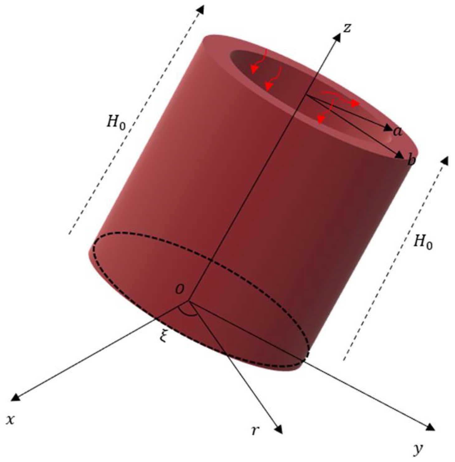
We consider a thermoelastic body to be an infinitely hollow cylinder made of a homogeneous transversely isotropic material with finite conductivity that has an inner radius
and an outer radius
and is free of traction (see
Figure 1). It begins in an undisturbed state at a uniform temperature
when a time-dependent symmetric thermal shock is applied to its inner surface while the outer surface is thermally insulated. We suppose that
denote the cylindrical polar coordinates, where the
-axis coincides with the cylinder axis. There are only two variables to consider in this problem: the distance variable,
, and the passage of time,
, due to the cylindrical symmetry of the problem.
As a result, the displacement vector involves the following components:
Using this displacement field, the corresponding strain components are derived as:
Therefore, the cubic dilatation,
, can be expressed as
The components that make up the mechanical stress tensor,
, can be deduced as follows:
where
,
, and
represent the normal thermal stresses.
In cylindrical coordinates, the following is the motion equation when external body forces are present:
where
represents the Lorentz force due to the presence of the magnetic field, which can be determined from the following relationship:
We take into account that the applied initial magnetic field,
, and the induced magnetic field,
, have the following components:
These equations clearly show that the non-vanishing components of vectors
and
only exist in the
-direction, i.e.,:
A linearization of Ohm’s law (11) yields:
In our situation, we can obtain the following two equations from Equation (9):
In the free space surrounding the cylinder, we can obtain the following two equations:
where
and
denote, respectively, the component of the electric field intensity and the induced magnetic field in free space surrounding the cylinder in the
-direction.
By removing variable
from Equations (20) and (21), we arrive at:
Again, when we remove
from Equations (21) and (23), and we obtain:
where
denotes the Laplace operator.
In our case, the radial component of the Maxwell stress tensor,
, is determined by:
The equation that describes the body force (Lorentz force) in the radial direction is as follows:
When Equations (15), (16), and (26), respectively, are used, the motion equation has the form:
Given that
for a transversely isotropic body, we may derive the following equation by applying the div operator on both sides:
In addition, the modified Moore–Gibson–Thompson heat conduction equation (MGTTE) (8) may be written as:
The following non-dimensional variables are used to simplify the system equations:
After removing the dashes for simplicity, the governing Equations (22)–(24), (27), and (28) may be reduced to:
where:
Parameter is an indicator of magnetic viscosity, while denotes the light speed. If , , and are all equal to zero, the above formulations simplify the standard generalized thermoelasticity equations without including magneto-electric influences.
In addition, the non-dimensional constitutive equations may be expressed as:
where:
5. Problem-Solving Approach Using Laplace Transform
Many areas of practical mathematics benefit significantly from the Laplace transform approach. Functions, measurements, and distributions are just a few of the numerous things that may be used to create it. After transforming Equations (31)–(38), using the Laplace transform under the starting conditions given in Equation (40) leads to:
where:
The following sixth-order differential equation is fulfilled by
after removing
and
from Equations (51)–(53):
where:
The factorization of Equation (36) yields:
where
,
, and
denote the solutions to the following characteristic polynomial:
The following is a valid representation of the solution to the Bessel Equation (57), which can be expressed as:
where
and
are the first and second kinds of modified Bessel functions of order zero, and
and
, with
, are some parameters that depend only on
.
We may write the following solutions similarly:
Equations (52) and (53), which are compatible with these equations, provide:
When Equation (59) is substituted into Equation (14), which is integrated concerning
, it yields the following result:
Displacement
can be derived using the Bessel function’s well-known relations, which are as follows:
When we enter the values from Equations (61) and (63) into Equation (47), we obtain:
The induced fields in free space,
and
, are obtained by removing
between Equation (48) to yield:
Equation (49) has a solution that is limited at the origin and at infinity, respectively, and is provided by:
where
and
denote the integration parameters.
Using relationship (64) and incorporating Equation (65) into (48), we obtain:
When both sides of Equation (44) are differentiated for
, we obtain:
When Equations (60), (63), and (71) are substituted into Equation (49), the components of the stress tensor are given as:
After substituting Equation (63) into (50), we obtain:
After applying the Laplace transforms, the boundary conditions (41)–(46) are converted to:
Substituting the solution functions into the above boundary conditions (Equations (60), (61), (65), (67)–(70), and (72)) yields a linear system of equations with unknown parameters, , with , and , with . By solving this system, the values of these constants can be set. As a result, an integrated solution to the problem is achieved in the field of the Laplace transform. Now, we have to find the inverse transformations of the solutions of the studied system domains to the space–time domain.
7. Graphical Results and Discussion
For computational reasons, a material with physical constants that is transversely isotropic is proposed. We consider a numerical case for which numerical solutions are offered to illustrate the previously supplied analytical approach and contrast the theoretical conclusions from the preceding sections. A numerical computation is created using the Mathematica software package. The physical constants of magnesium (Mg) are listed as follows [
31]:
In the calculations, we use the inner radius of the cavity as ; the outer radius as , with respect to the center of the hole; and one value of time () unless otherwise specified.
In three scenarios, numerical computations are performed. The first scenario examines how the non-dimensional field variables fluctuate with the magnetic field, while time and relaxation time stay constant. The second objective is to examine how non-dimensional temperature change , radial displacement , and thermal stresses ( and ) fluctuate for various thermoelastic models while time remains constant. The third instance investigates how the studied non-dimensional fields fluctuate with time while all other parameters are held constant. The numerical results of the fields of study are represented in tables and figures for the purpose of comparison and the discussion of the problem.
7.1. The Effect of the Applied Magnetic Field
Because it can be used in many different fields, including Earth sciences, plasma physics, nuclear engineering, and other similar topics, the mechanical properties and how electromagnetic forces, temperature, pressure, and strain affect each other in a thermoelastic material are very important topics of investigation. The ability of magnetic materials to exhibit reversibility, that is, the production of electric charge in response to an applied mechanical force and the internal generation of mechanical vibration in response to an applied electric field, are among their greatest properties. Due to their intrinsic properties, magnetic materials are widely used in the fields of electrical and electronic engineering, structural engineering, medical equipment, and contemporary industry.
The present section focuses on studying thermoelasticity waves in a hollow, flexible cylinder that conducts electricity and has a stress-free boundary. The cylinder is placed inside a magnetic field surrounding its inner surface. While maintaining constant relaxation time (
) and transit time (
) parameters, the first situation is a study of non-dimensional investigated field variables using the proposed generalized Moore–Gibson–Thompson thermoelasticity (MGTTE) model in the presence
and absence of the electromagnetic field effect
. If parameters
,
, and
, which are defined in equation (36), are all equal to zero, the generalized thermoelasticity equations do not include magneto-electric influences. Changes in the spatial coordinates can be seen in
Figure 2,
Figure 3,
Figure 4,
Figure 5 and
Figure 6.
It is clear from the curves in the figures that the nature of the variation in the fields varies with time. The data clearly show that the applied magnetic field significantly affects each field under investigation. The phenomenon of finite propagation velocity is also found in all figures. On the other hand, the propagation speed in the case of the coupled and uncoupled classical theories of thermoelasticity is infinite; all the functions involved have infinite values at every point in the medium away from sources and thermal shocks.
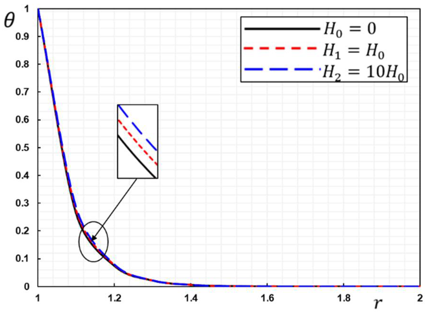
The variation in temperature c across the radial distance is shown in
Figure 2. The temperature changes are initially of larger magnitudes and become smaller over time to ensure that they meet the boundary requirements, as shown in
Figure 2. In addition, for all values of
, it goes down quickly as the distance from the center increases and goes away before
. The heat wave front moves forward over time at a finite pace. The graph shows that only in a finite space field at a given moment, the temperature has a non-zero value. Thermal oscillation is sensed in the region close to the heat shock, and the turbulence disappears outside this region. In many locations, the non-zero region moves all the time, consistently. Although the magnetic field has a slight effect on the temperature distribution, it helps to increase the amount of temperature change.
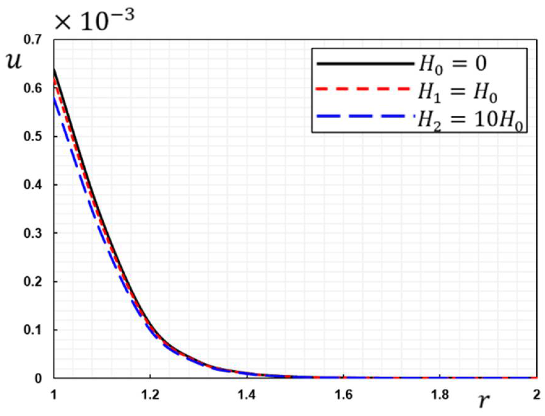
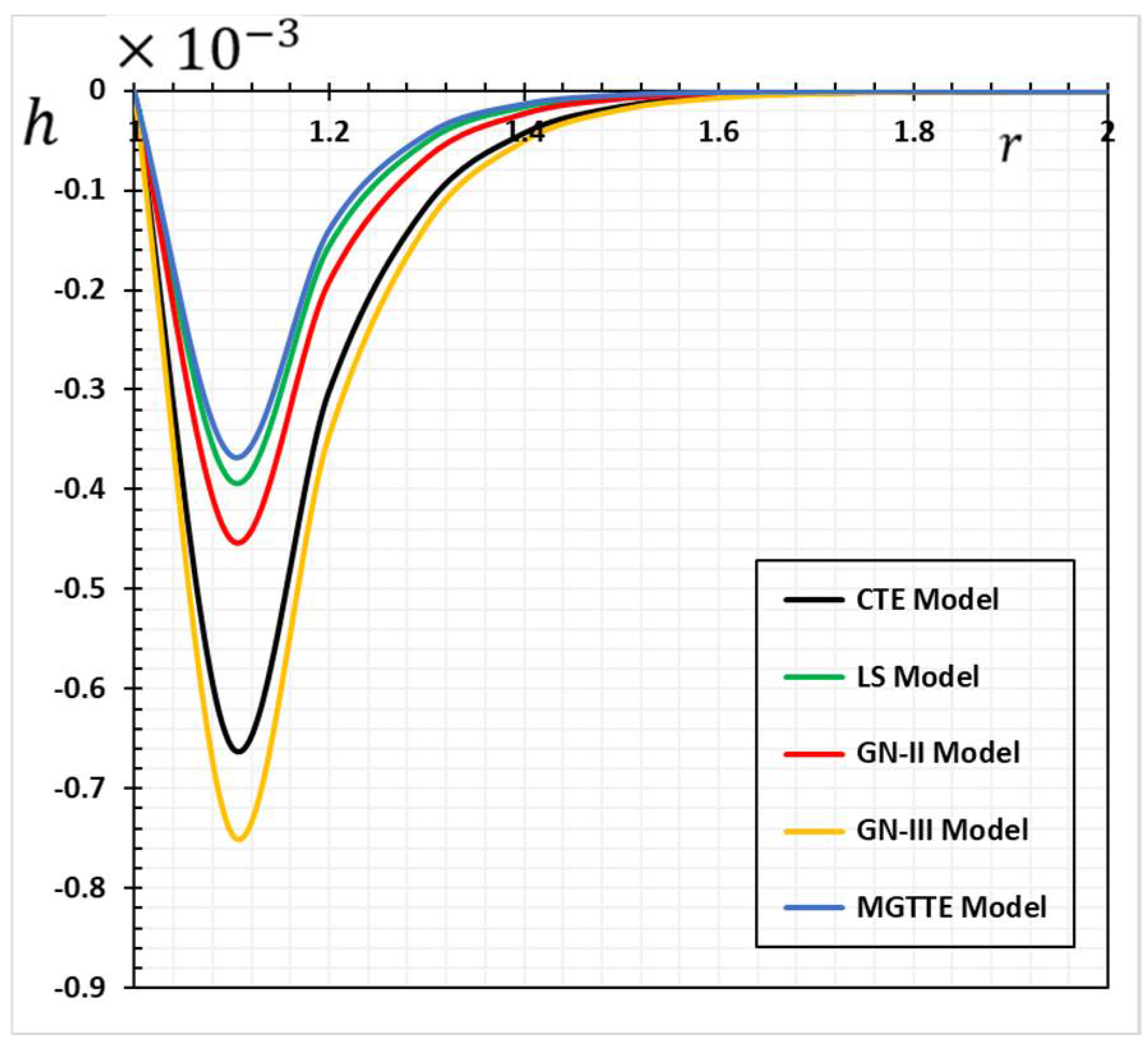
Figure 3 represents the variation in radial displacement
versus radial distance
for different values of the magnetic field.
Figure 3 depicts the displacement variation, starting with positive values in all situations and decreasing to zero over time. This distortion is the result of a dynamic phenomenon. When magnetic field
values increase, we see a decrease in the magnitudes of the displacement. It can be seen from
Figure 2 that the wave effect limits the temperature of the non-zero region of the radial displacement at a given moment. Over time, it appears that heat is transmitted to the deeper layers of the medium at a limited rate. The thermal turbulence and the radial displacement area go up directly with the investigated moment.
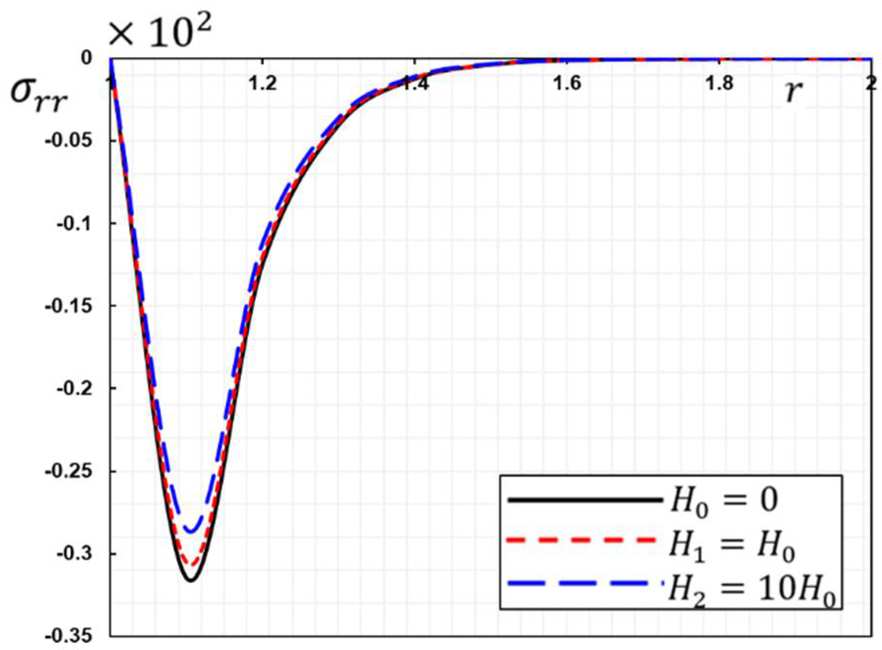
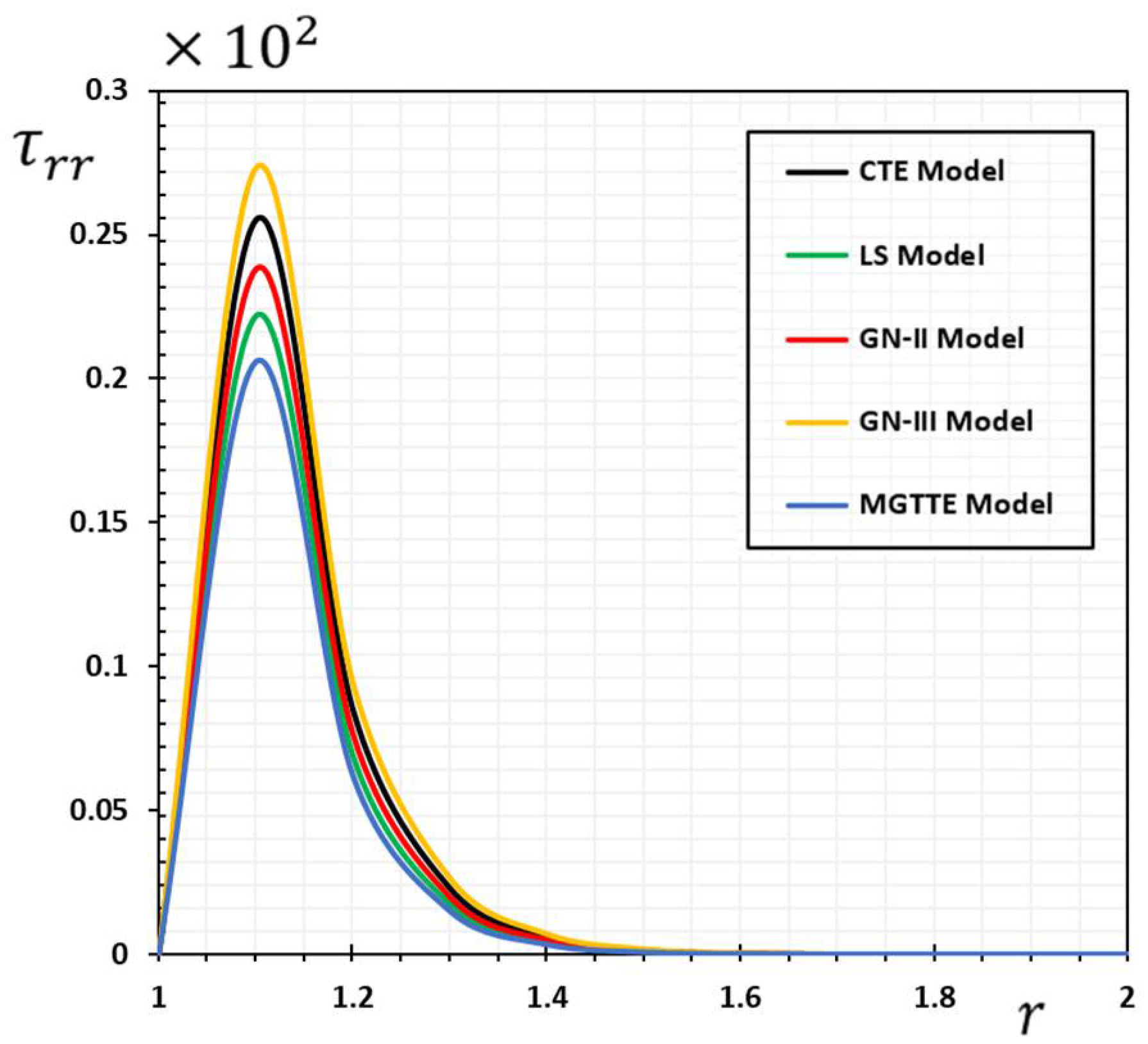
Figure 4 shows how radial tension
varies with redial position
in each example. It should be noticed that radial stress
rapidly rises to zero values after immediately decreasing from zero to a minimum value. As can be seen in
Figure 4, thermal stress
fluctuations at the side walls of the hollow cylinder with
and
correspond to the boundary conditions, as they always start and end with zero values. The values of initial magnetic field
raise pressure
, which is another observation that can be gleaned from the graph. The tension affects the material on the inner surface of the cylinder. This change corresponds to the radial expansion deformation of the medium, as in
Figure 3. In addition, it is observed that the compressed region shrinks with time, and the tensile stress region grows, which is consistent with the previously mentioned dynamic stretching effect.
Figure 4 also shows that the area of non-zero stress is limited at some point near the heat shock. This shows how temperature waves affect the current change in stress
.
Elastic elements and systems subjected to mechanical loads while immersed in a magnetic field with a large energy variation can experience a wide range of stresses. The generated electrodynamic losses add thermal stress, and the Lorentz force adds magnetic stress to the already present mechanical stress. As well as influencing one another, these stressors are very complicated. Validating the current conclusions requires closely fitting the new data to the prior data [
42]. This means that the accuracy of present numerical estimates is quite good.
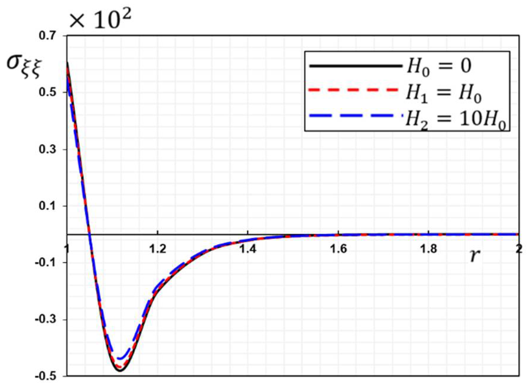
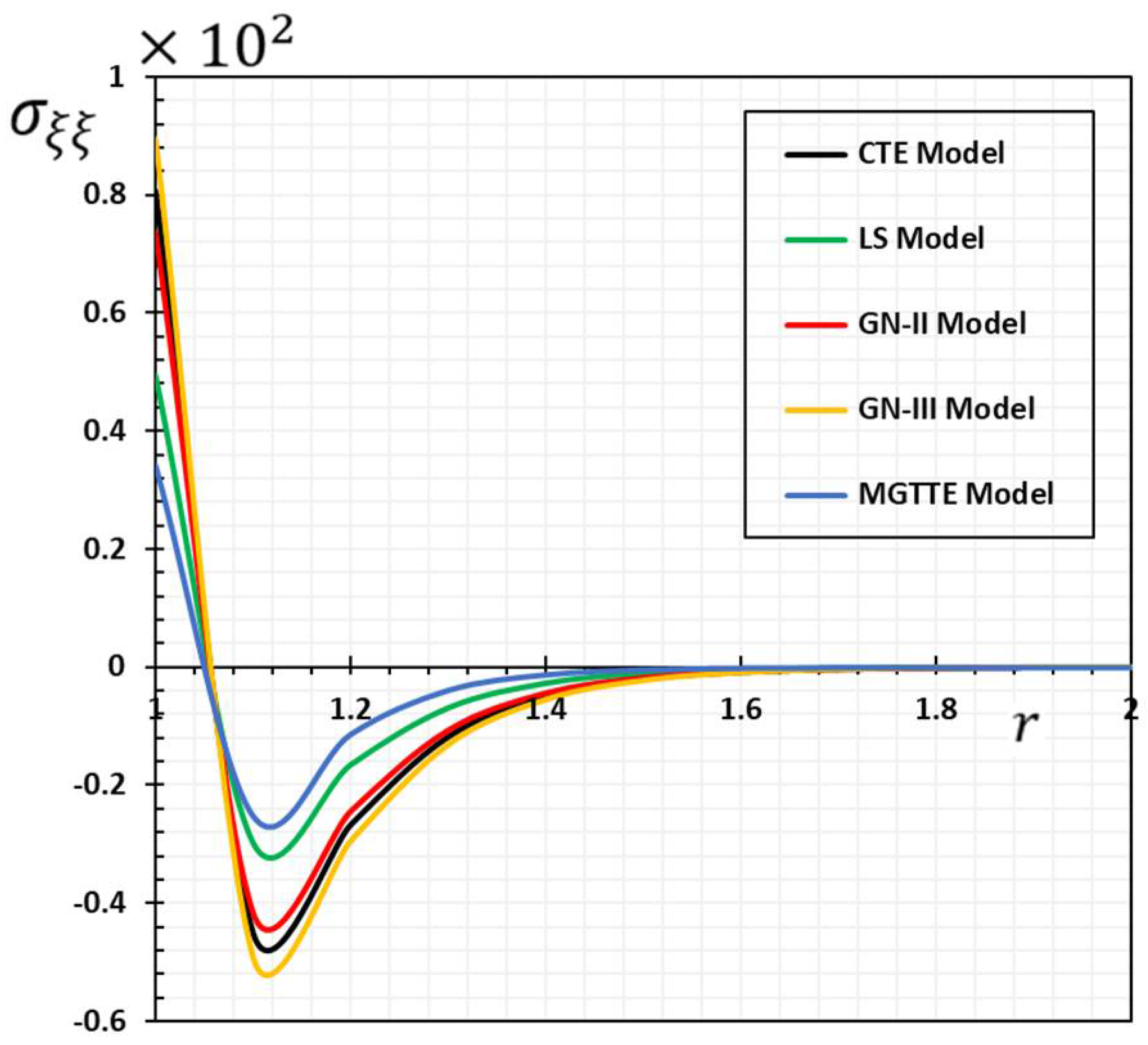
Figure 5 depicts the behavior of hoop stress
as the radial distance changes with and without the effect of initial magnetic field
changing. As the illustration shows, there is circumferential compressive stress for the transversely isotropic material. It is also clear from the figure that the behavior of circumferential stress
is the same as that of radial stress
, but the difference is in the starting point, where the hoop stress starts with positive values different from zero. Compression occurs in one section of the cylinder, while tension occurs in another, as shown in
Figure 4 and
Figure 5. The area close to the inner surface of the cylinder undergoes increasing tensile stress over time as it fades to the other side. From
Figure 4, we can find that the amount of stress
increases as the magnetic field immersing the cylinder increases. This shows that the effect of parameter
develops further into the hollow cylinder, in addition to the effect of thermal shock.
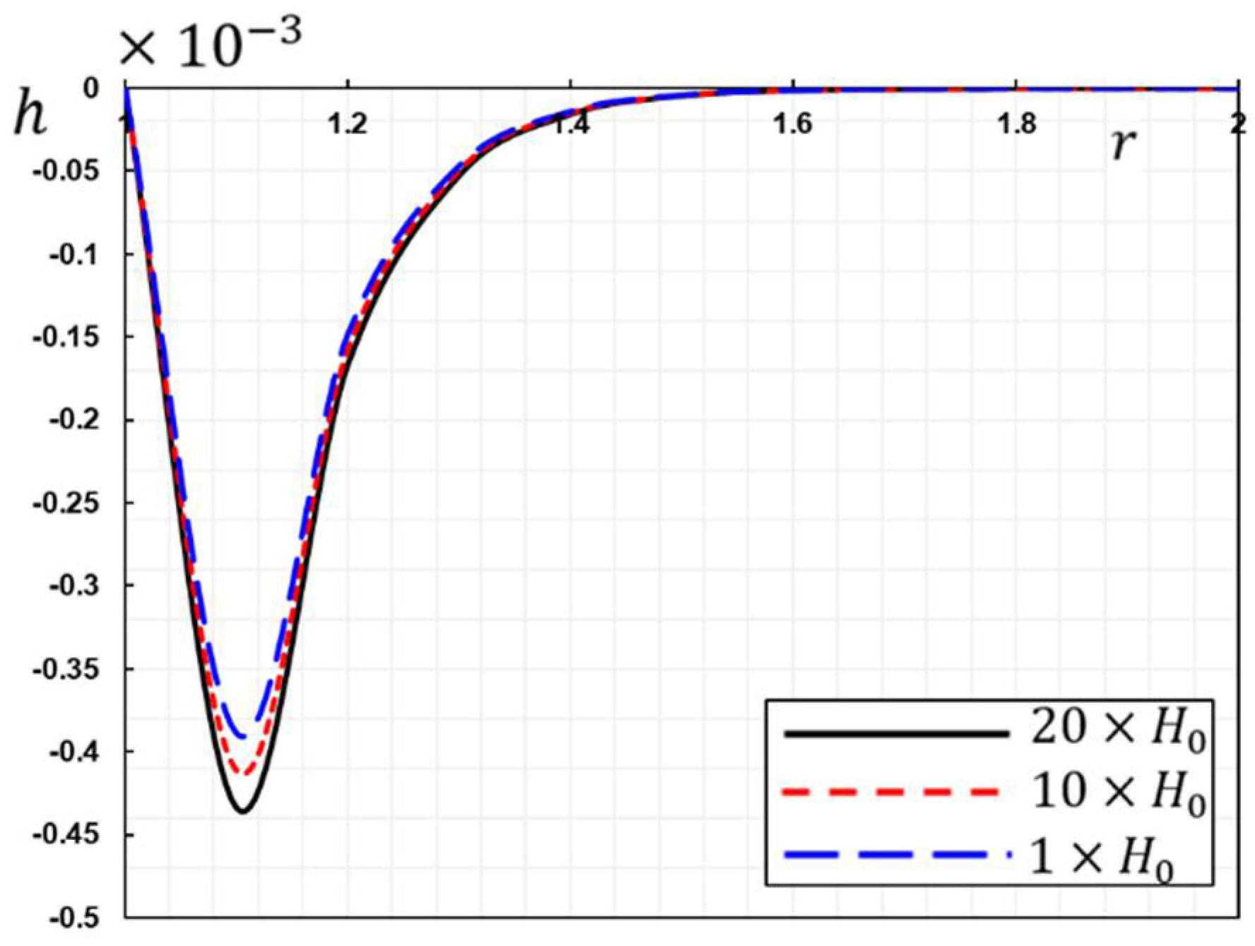
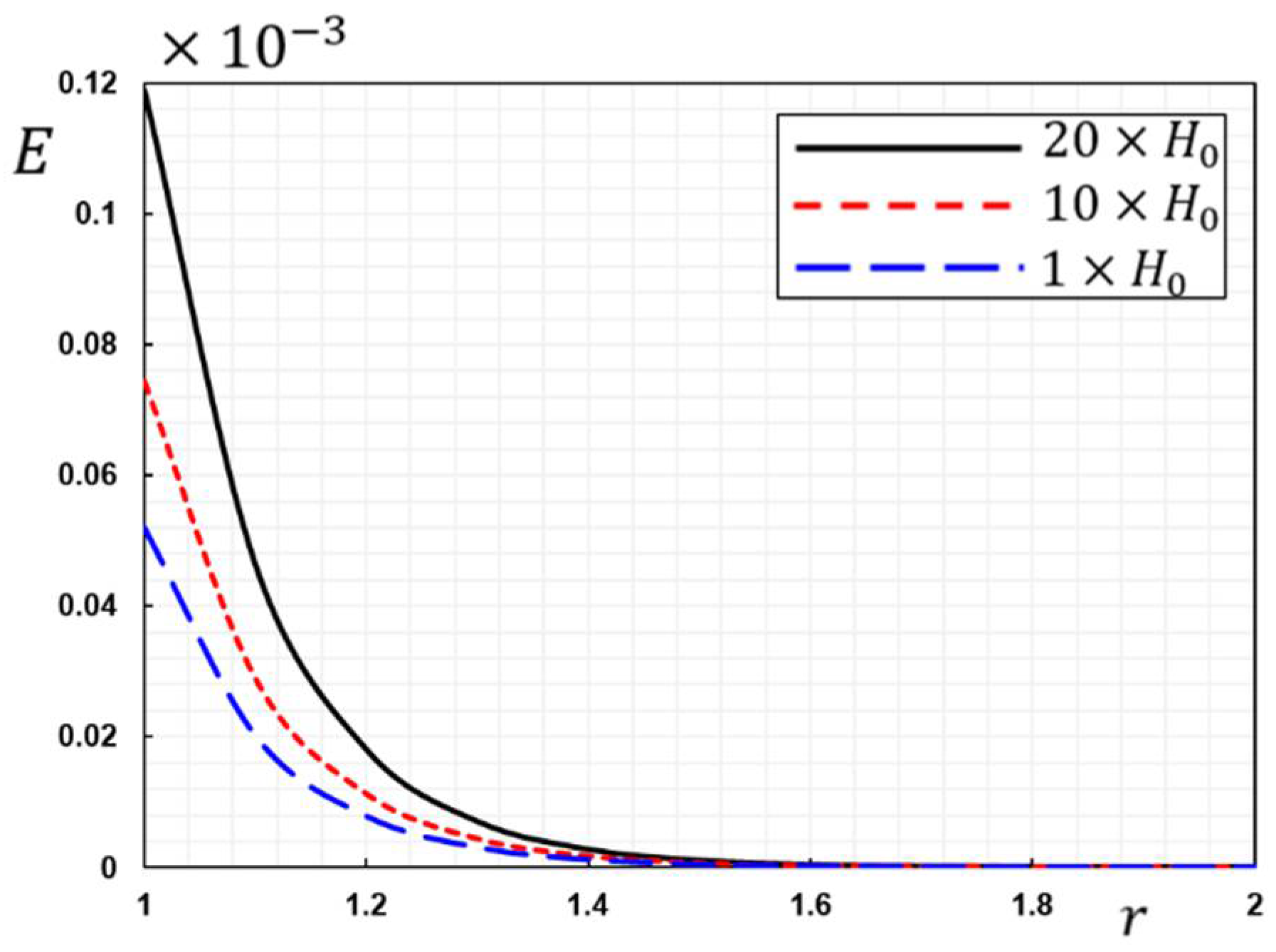
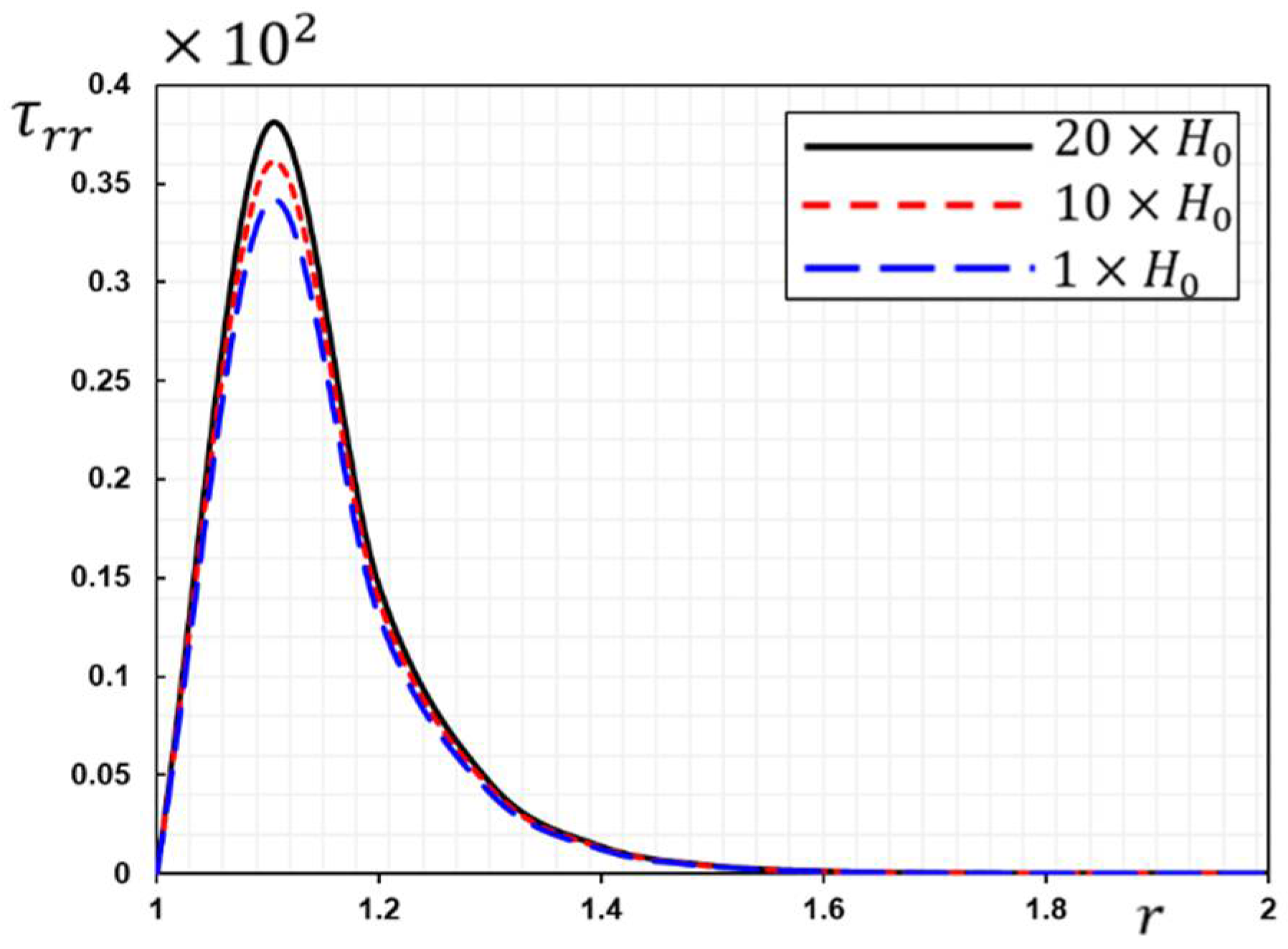
Figure 6,
Figure 7 and
Figure 8 depict non-dimensional induced magnetic field
, induced electric field
, and the radial Maxwell stress
distribution in the hollow cylinder with three different values of axial magnetic field
. The associated thermo-elastic and electromagnetic interactions can be easily found in
Figure 6,
Figure 7 and
Figure 8. Thermal shock causes the deformation of the electromagnetic medium, which is initially in a magnetic field. As a result, the magnetic flux passing through the cross-section of the cylinder changes. Thus, the medium contains an induced magnetic field in addition to an induced electric field. As the heat wave moves deeper into the cylinder, the magnetic and electric fields that it creates change. This is further proof that heat moves in a waveform.
According to the figures and numerical results, the coefficient of variation in axial magnetic field
has a significant effect on the behavior of all induced fields, whether electric or magnetic, which increases the importance of considering the effect of axial magnetic field
. It is clear from looking at
Figure 6,
Figure 7 and
Figure 8 that when
is equal to
and
, the absolute values of all the field variables are higher than they are when
is equal to
.
Thermo-magneto-elastic investigations of plates and shells have previously heavily relied on linear models and simplified ideas. In reality, however, most plate and shell constructions are subjected to high-energy, temperature-varying electromagnetic radiations, resulting in strongly coupled deformations [
43]. Sheets and circular panels are used in engineering for things such as pneumatics, turbine diaphragms, marine structures, nuclear reactors, optical systems, shipbuilding, cars and other vehicles, space shuttles, sound emitters and receivers, ports and swivel panels, and other annular tapers [
44].
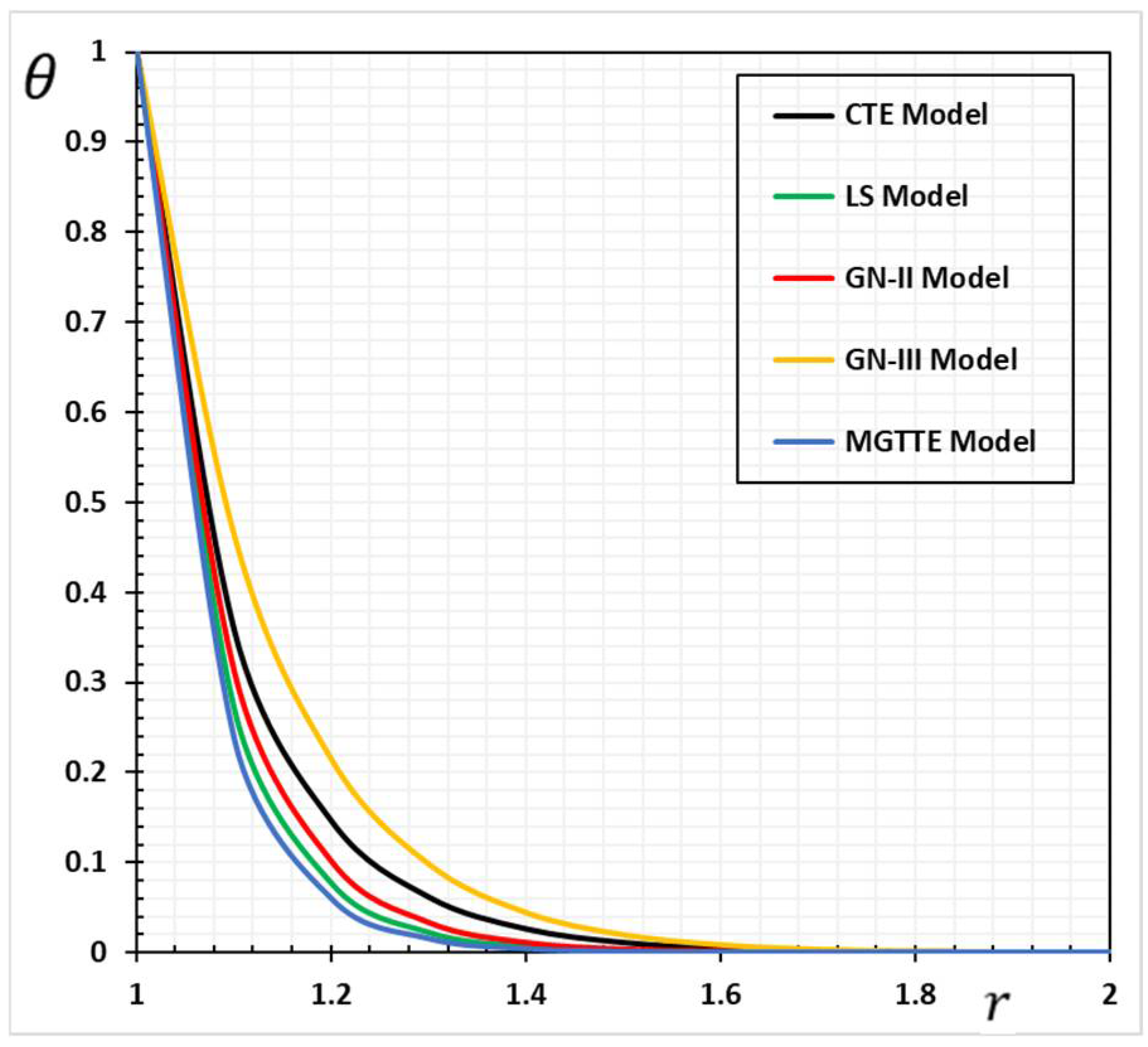
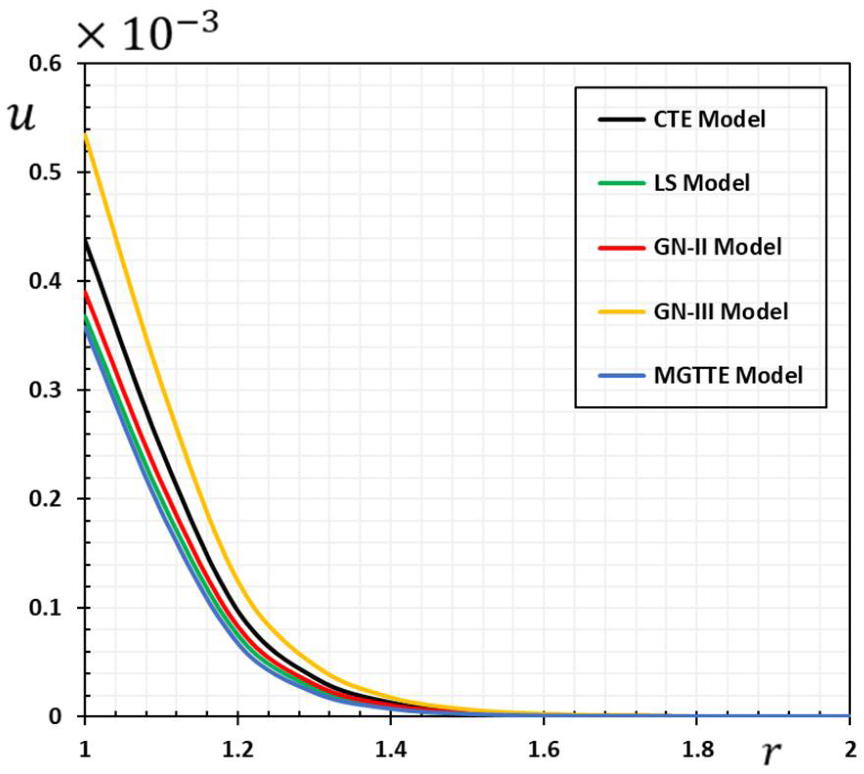
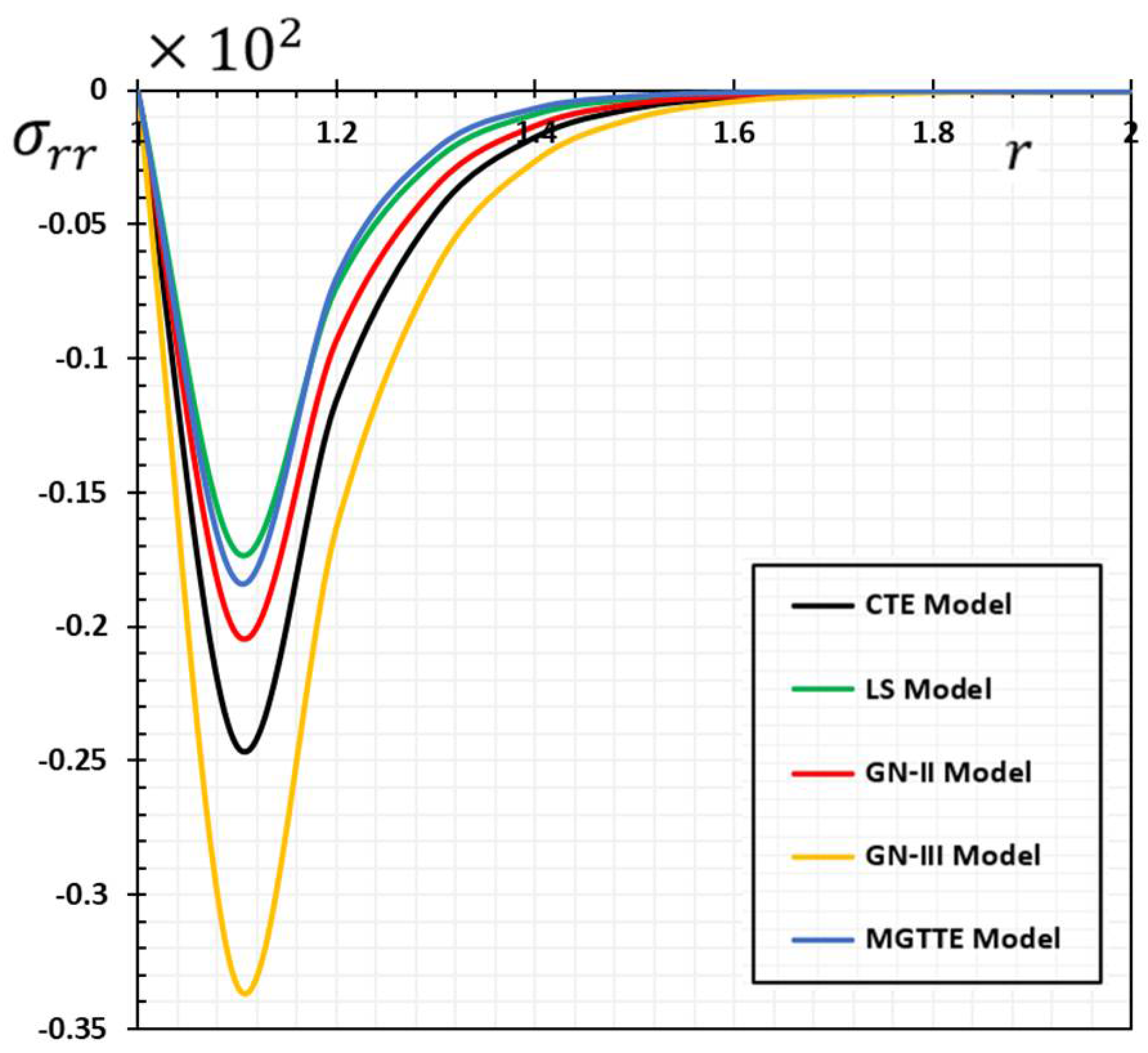
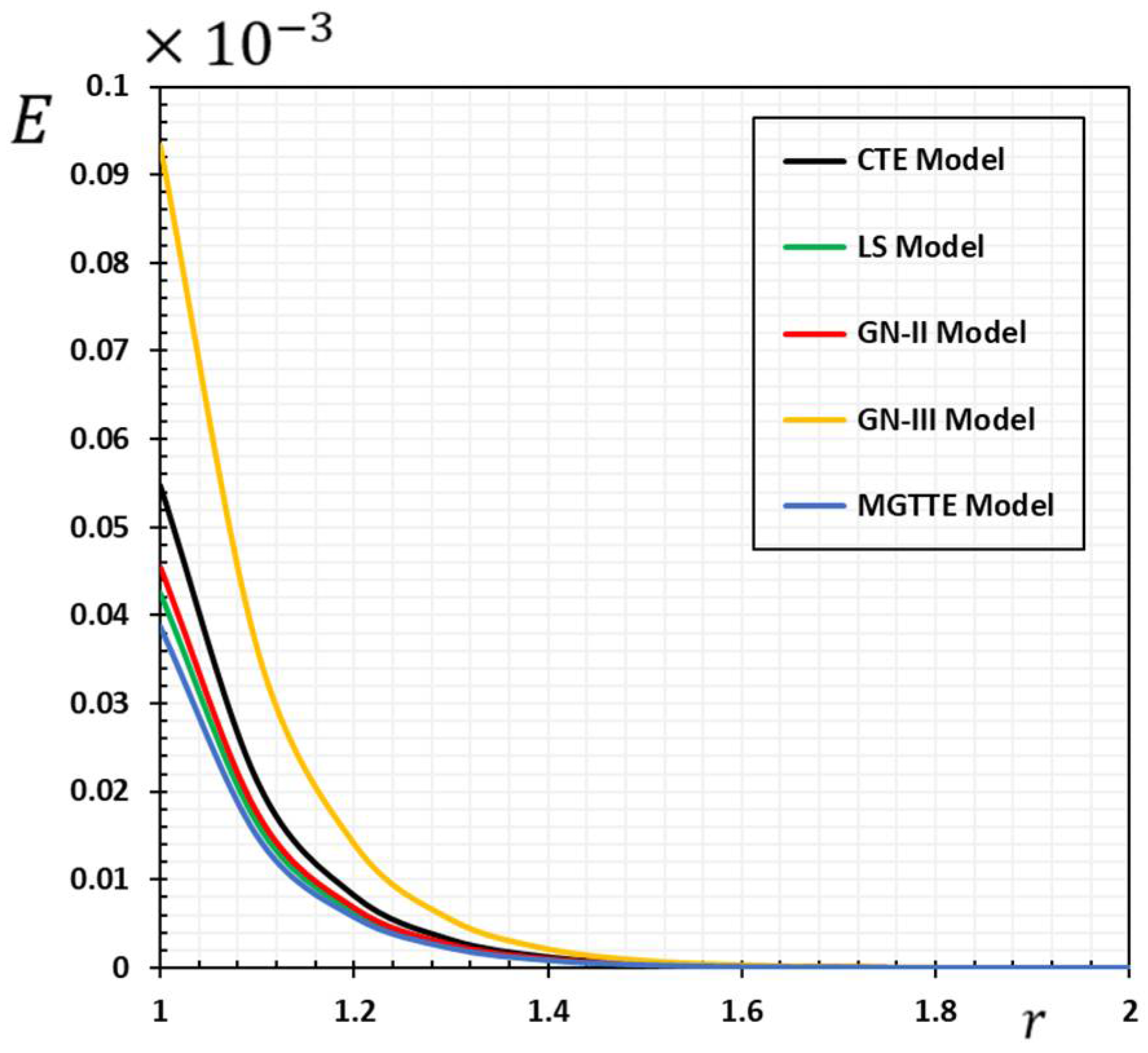
7.2. Comparison of Different Models of Thermoelasticity
In the second scenario of this discussion, the behavior of non-dimensional thermal and mechanical field variables as well as electromagnetic variables versus radial distance
are explored in the case of various thermoelastic theories. In this case, axial magnetic field
and time
remain the same.
Figure 8,
Figure 9,
Figure 10,
Figure 11,
Figure 12,
Figure 13 and
Figure 14 depict a different variant of the physical fields each to illustrate the differences between the different theories of thermoelasticity and their relationship to each other. The model proposed in this article presents many previous models in the general thermoelastic theory as special cases. The coupled dynamical thermoelasticity theory (CTE) can be obtained when
, while the Lord–Shulman model (LS) is in the case of
. In addition, the second type of the Green–Naghdi theorem (GN-II) can be derived when the term that includes parameter
is equal to zero and there is no thermal relaxation time. On the other hand, when neglecting the thermal relaxation time, the third type (GN-III) can be produced. In the presence of thermal relaxation
, and
and
parameters, we have the Moore–Gibson–Thompson generalized thermoelastic theory (MGTTE).
This subsection presents the results in
Table 1,
Table 2,
Table 3,
Table 4,
Table 5,
Table 6 and
Table 7 and
Figure 9,
Figure 10,
Figure 11,
Figure 12,
Figure 13,
Figure 14 and
Figure 15, aiming to facilitate comparisons between different thermoelastic models. Future scientists can compare their results using the tables in this article. Looking at the tables and noting
Figure 5,
Figure 6,
Figure 7 and
Figure 8, it can be seen that the thermal parameters strongly influence the distribution of the studied field quantities,
and
. It is also evident that the values of the fields vary with different thermal models. Both the generalized (LS, GNII, GNIII, and MGTTE) and coupled (CTE) thermoelastic models provide remarkably similar results in behavior near the inner cylinder surface where the boundary conditions imposed by the proposed problem are present. The findings, which are consistent with generalized thermoelasticity theories, are extremely comparable as the distance rises.
In contrast with generalized thermoelastic models, which assume that heat waves move at a limited speed, the coupled theory says that heat waves move at an unlimited speed. The numerical results show that the heat wave travels from the inside of the cylinder to the outside because the thermal shock is applied only to the inner surface of the cylinder.
Table 1,
Table 2,
Table 3 and
Table 4 and
Figure 9,
Figure 10,
Figure 11,
Figure 12,
Figure 13,
Figure 14 and
Figure 15 show the discrepancy between the predictions of the GN-III model and the MGTE model. The results show that the numerical values and curves in the case of the GN-III model are greater than the values and fields of the curves in the case of the MGTE model. It is also noticed that the numerical values of both the LS and MGTE models show similar results and behaviors. The reason for this is that there is a thermal relaxation time. The results of the Green and Naghdi type III thermoelastic model (GN-III) show that they differ significantly from the small energy dissipation type II thermoelastic concepts (GN-II) [
16,
27]. When comparing the GN-II model with other models, it can be seen that the temperature values and distributions are very different.
These illustrations clearly show that the waves propagate at limited rates in the extended Moore–Gibson–Thompson thermoelasticity theory (MGTTE). We see that all variables disappear uniformly outside a time-varying, finite region. This is not true for coupled thermoelasticity (CTE) and Green and Naghdi type III, where the function under consideration has non-vanishing values for all values of
because heat waves spread at an unlimited rate. Compared with previous generalized models of thermoelasticity, the results of GN-IIII show convergence with the classical elasticity model (CTE) results, which do not fade quickly under the influence of heat inside the medium. This matches perfectly with the information provided by Quintanilla [
25], which is why the new model is proposed in this article.
8. Conclusions
The main objective of the present work is to investigate the effects of a detailed analysis of thermally induced and mechanical vibrations of a transverse, thermoelastic, long, hollow cylinder under the proposed Moore–Gibson–Thompson (MGTTE) thermoelastic model. The governing equations of the system are solved using the Laplace transform method to figure out the studied physical fields.
According to the results of the study, the most important conclusions can be summarized as follows:
The applied axial magnetic field significantly influences the increase or decrease in the researched field variables through the thermoelastic materials in the investigated fields. Nevertheless, it has a small influence on the non-dimensional temperature;
When electromagnetic radiation hits flexible structures, it creates different temperature differences and a lot of energy, which distorts the highly coupled medium;
In the expanded Moore–Gibson–Thompson thermoelastic model, thermal waves are dispersed as finite-velocity waves rather than infinite waves in a transversely isotropic material, as in the conventional thermoelastic theory. In addition, there was convergence and similarity between the GN-III and CTE models, which indicates the validity and relevance of the presented thermoelastic model;
Both the LS and MGTE models show similar results and similar behaviors. The reason for this is that there is a thermal relaxation time.
Finally, the methodology described in this article applies to many thermodynamic challenges. The diaphragms of turbines, aircraft and missiles, marine structures, nuclear reactors, optical systems, shipbuilding, automobiles and other vehicles, space shuttles, sound emitters and receivers, ports and rotating plates, and other annular structures are just a few of the engineering applications of these circular sheets and plates. Experimental scientists and researchers who study this field can also benefit from these theoretical findings.


