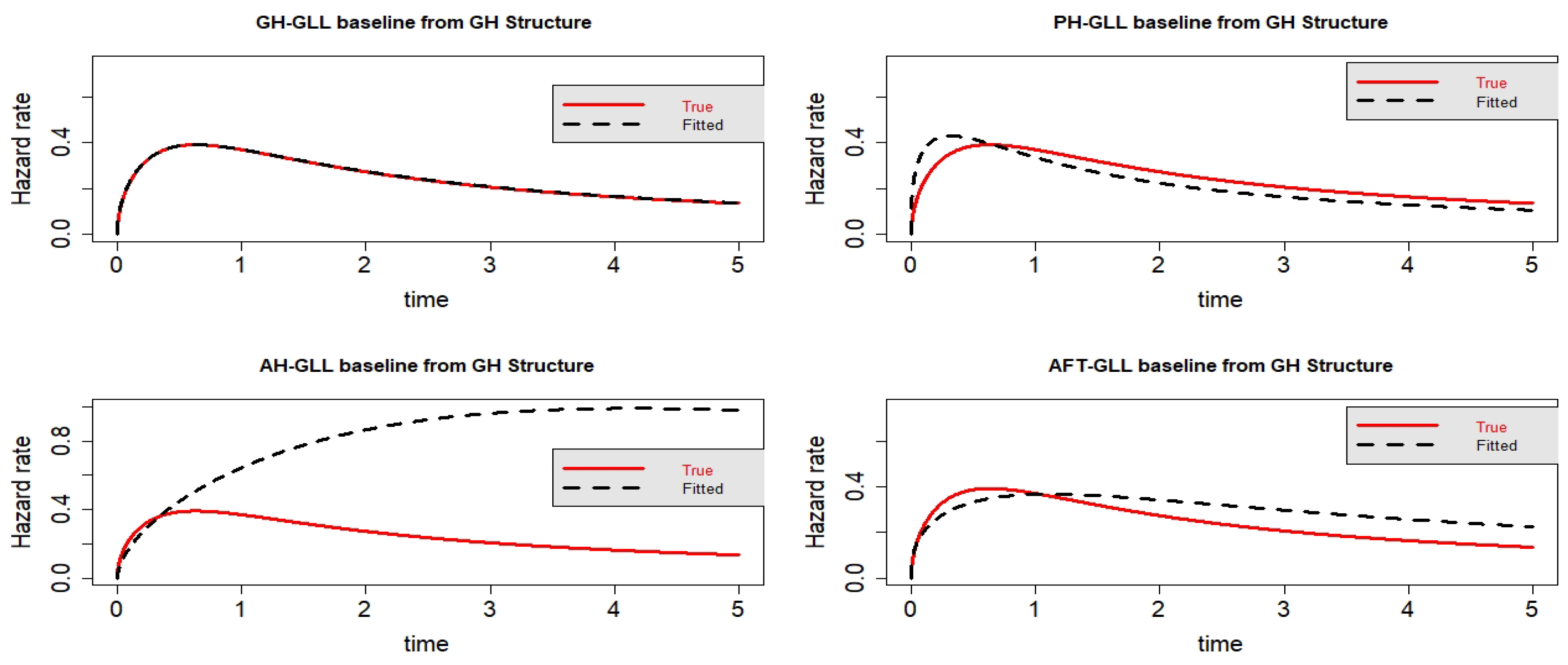
Figure 1.
Estimated baseline hrfs with censoring proportion of and a sample size of . The dashed and solid curves indicate the estimated and true hrfs, accordingly. The data generated from a GH structure.
Figure 1.
Estimated baseline hrfs with censoring proportion of and a sample size of . The dashed and solid curves indicate the estimated and true hrfs, accordingly. The data generated from a GH structure.
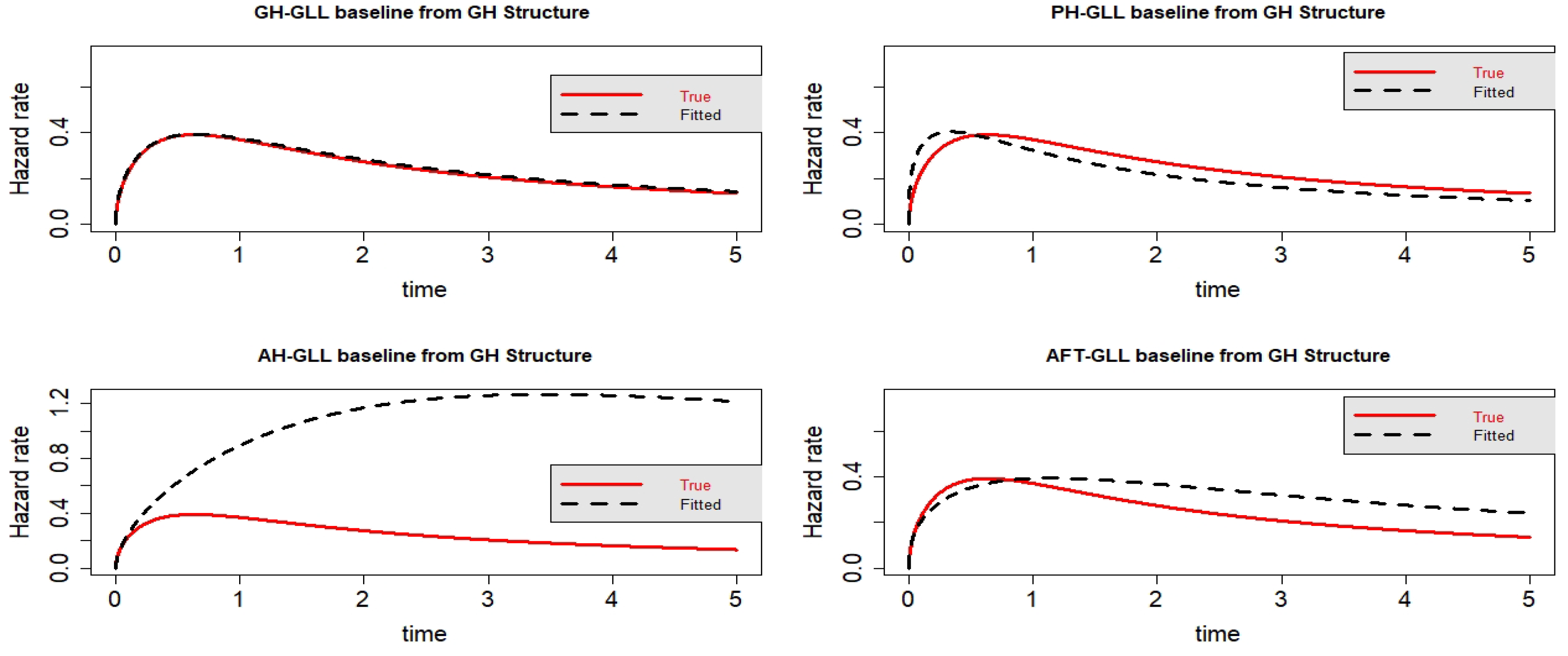
Figure 2.
Estimated baseline hrfs with censoring proportion of and a sample size of . The dashed and solid curves indicate the estimated and true hrfs, accordingly. The data generated from a GH structure.
Figure 2.
Estimated baseline hrfs with censoring proportion of and a sample size of . The dashed and solid curves indicate the estimated and true hrfs, accordingly. The data generated from a GH structure.
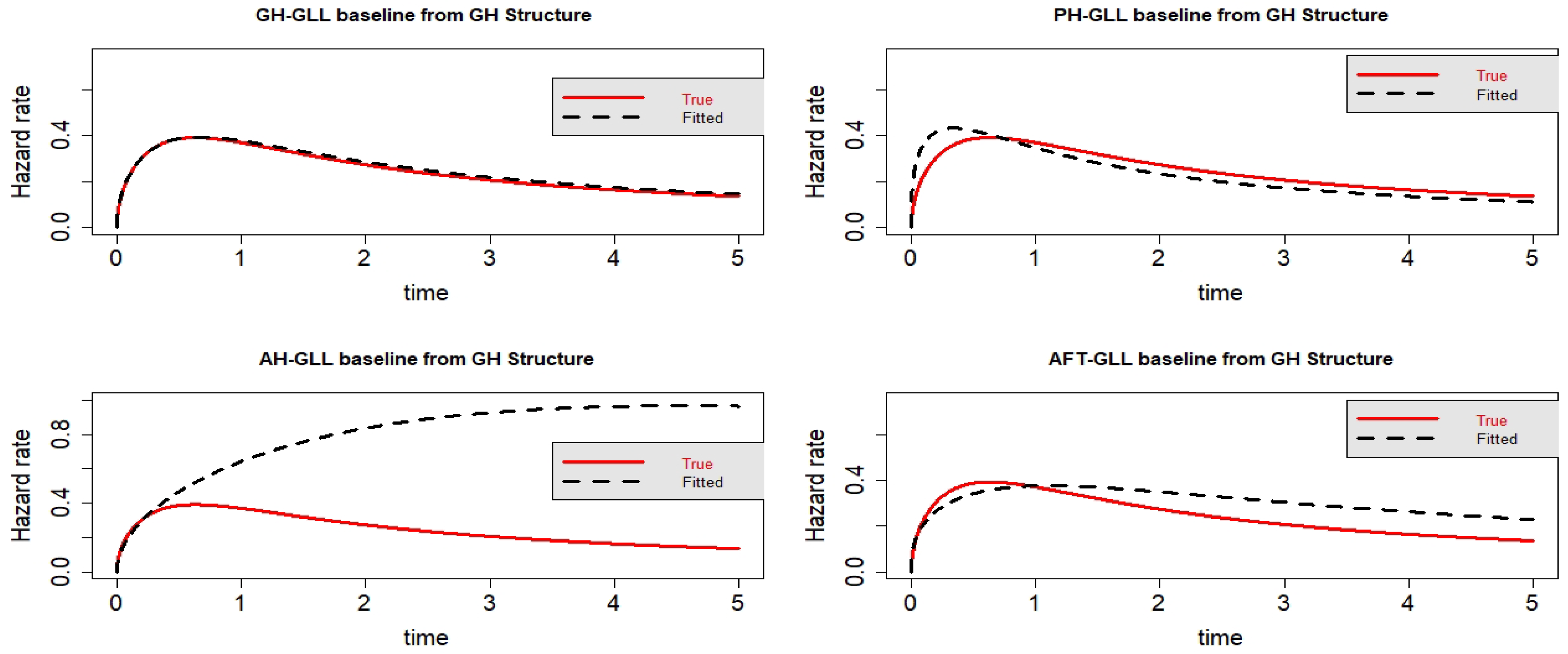
Figure 3.
Estimated baseline hrfs with censoring proportion of and a sample size of n = 10,000. The dashed and solid curves indicate the estimated and true hrfs, accordingly. The data generated from a GH structure.
Figure 3.
Estimated baseline hrfs with censoring proportion of and a sample size of n = 10,000. The dashed and solid curves indicate the estimated and true hrfs, accordingly. The data generated from a GH structure.
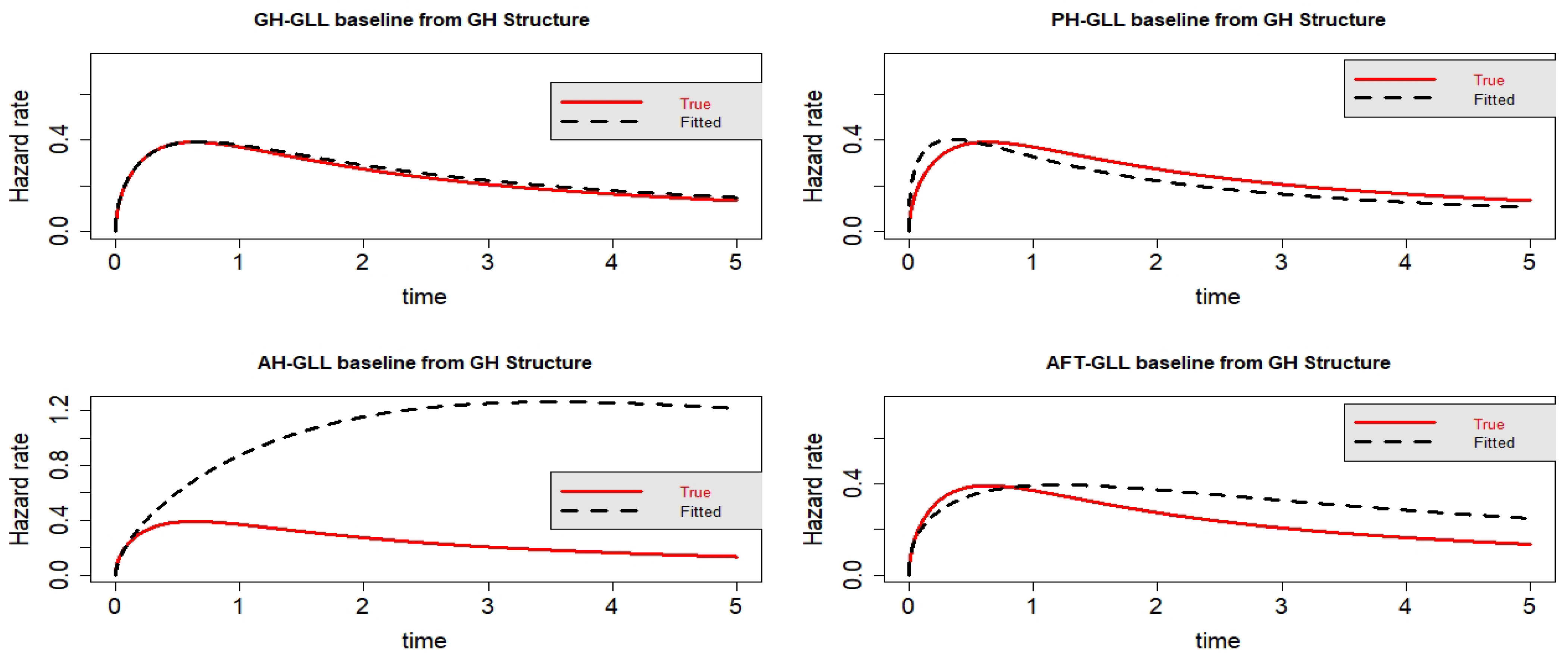
Figure 4.
Estimated baseline hrfs with censoring proportion of and a sample size of n =10,000. The dashed and solid curves indicate the estimated and true hrfs, accordingly. The data generated from a GH structure.
Figure 4.
Estimated baseline hrfs with censoring proportion of and a sample size of n =10,000. The dashed and solid curves indicate the estimated and true hrfs, accordingly. The data generated from a GH structure.
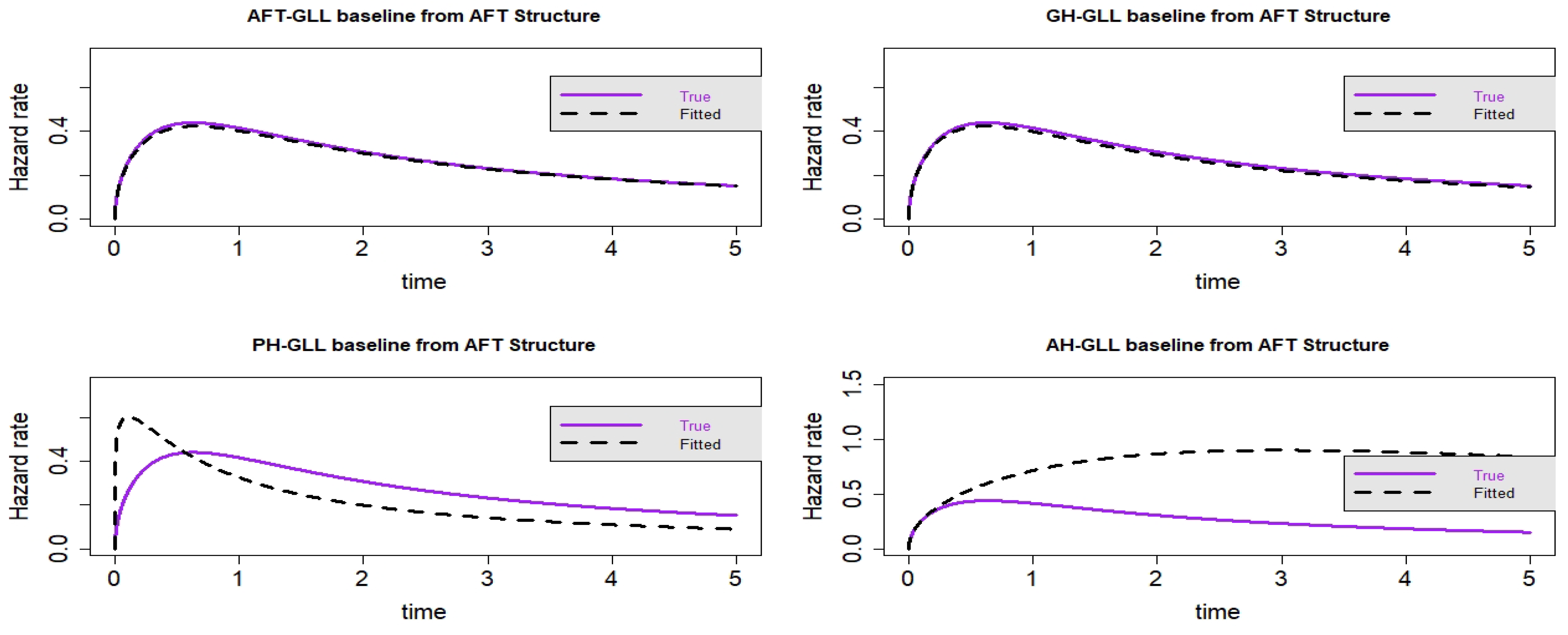
Figure 5.
Estimated baseline hrfs with censoring proportion of and a sample size of . The dashed and solid curves indicate the estimated and true hrfs, accordingly. The data generated from an AFT structure.
Figure 5.
Estimated baseline hrfs with censoring proportion of and a sample size of . The dashed and solid curves indicate the estimated and true hrfs, accordingly. The data generated from an AFT structure.
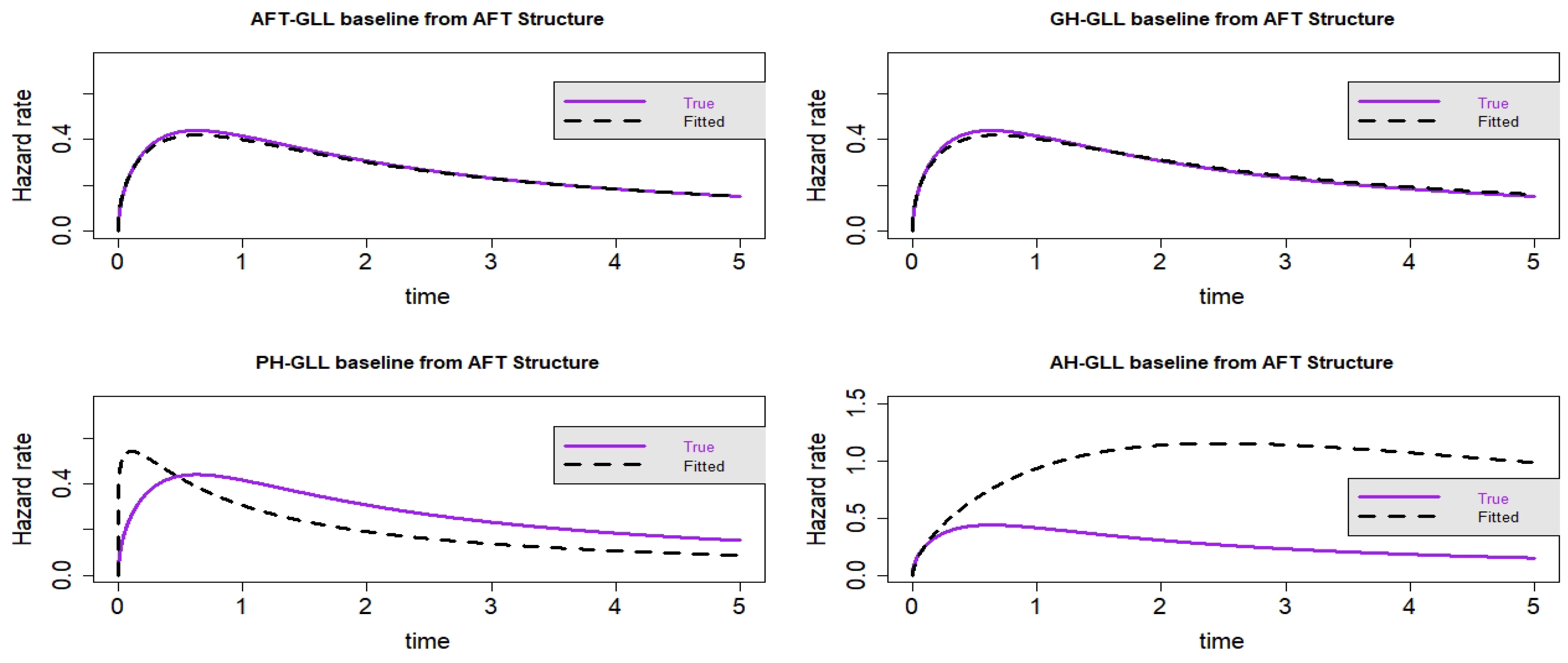
Figure 6.
Estimated baseline hrfs with censoring proportion of and a sample size of . The dashed and solid curves indicate the estimated and true hrfs, accordingly. The data generated from an AFT structure.
Figure 6.
Estimated baseline hrfs with censoring proportion of and a sample size of . The dashed and solid curves indicate the estimated and true hrfs, accordingly. The data generated from an AFT structure.
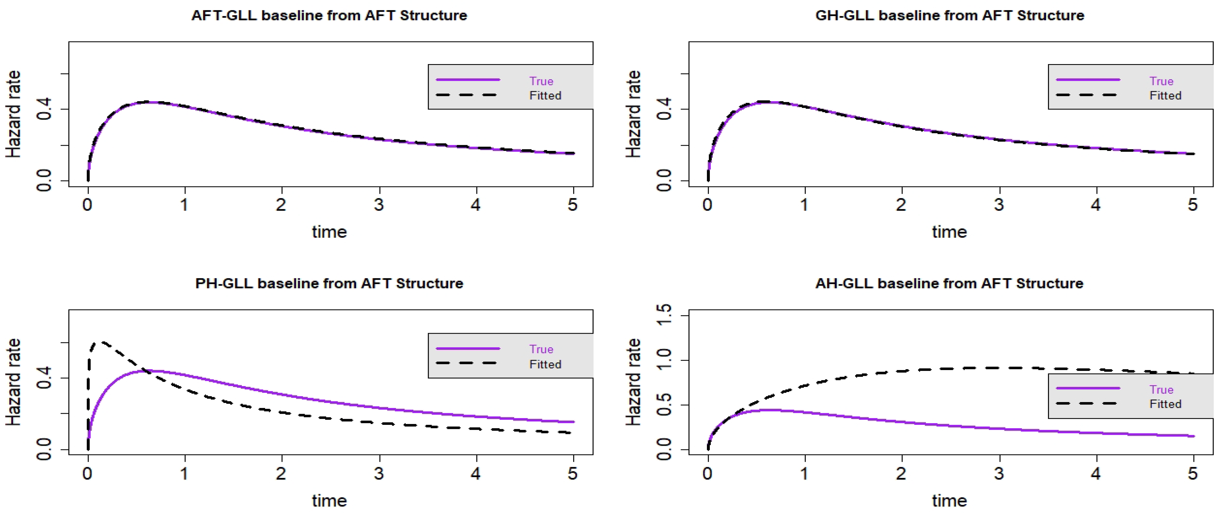
Figure 7.
Estimated baseline hrfs with censoring proportion of and a sample size of n = 10,000. The dashed and solid curves indicate the estimated and true hrfs, accordingly. The data generated from an AFT structure.
Figure 7.
Estimated baseline hrfs with censoring proportion of and a sample size of n = 10,000. The dashed and solid curves indicate the estimated and true hrfs, accordingly. The data generated from an AFT structure.
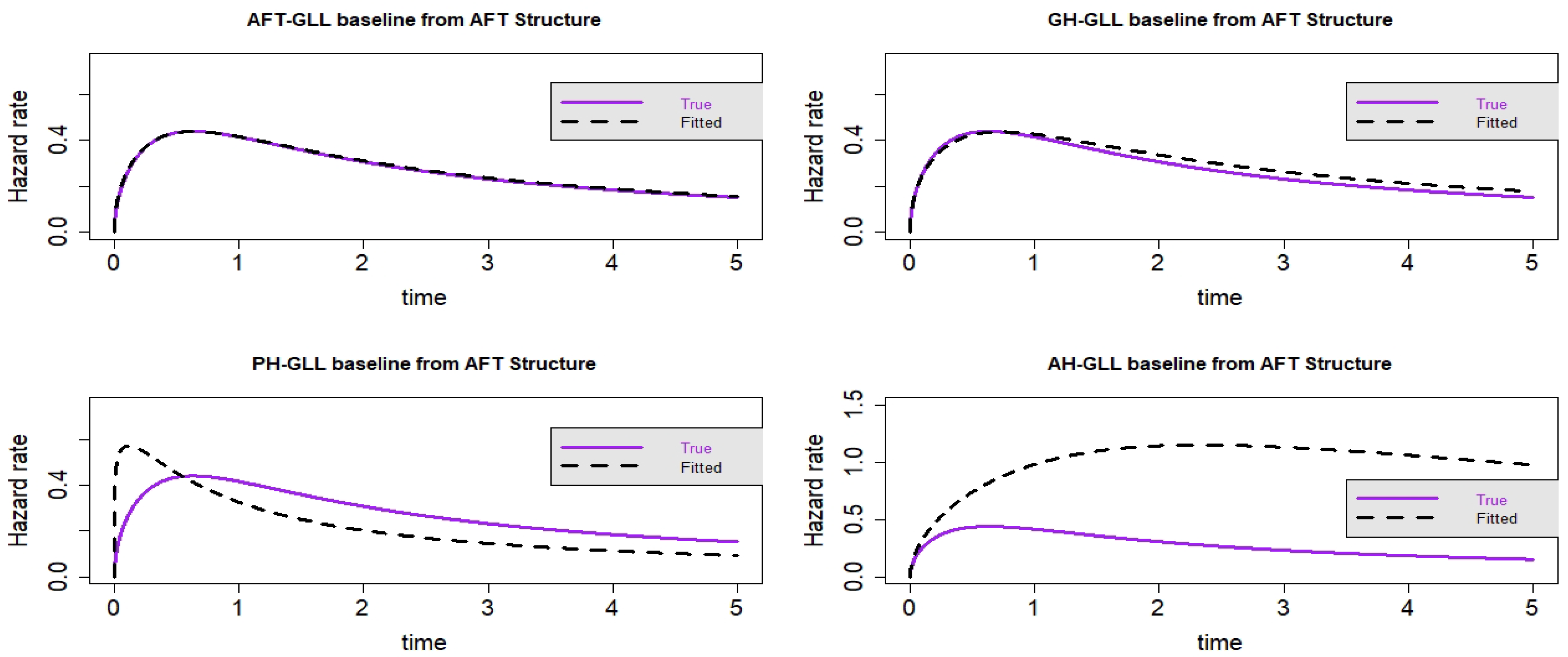
Figure 8.
Estimated baseline hrfs with censoring proportion of and a sample size of n = 10,000. The dashed and solid curves indicate the estimated and true hrfs, accordingly. The data generated from an AFT structure.
Figure 8.
Estimated baseline hrfs with censoring proportion of and a sample size of n = 10,000. The dashed and solid curves indicate the estimated and true hrfs, accordingly. The data generated from an AFT structure.
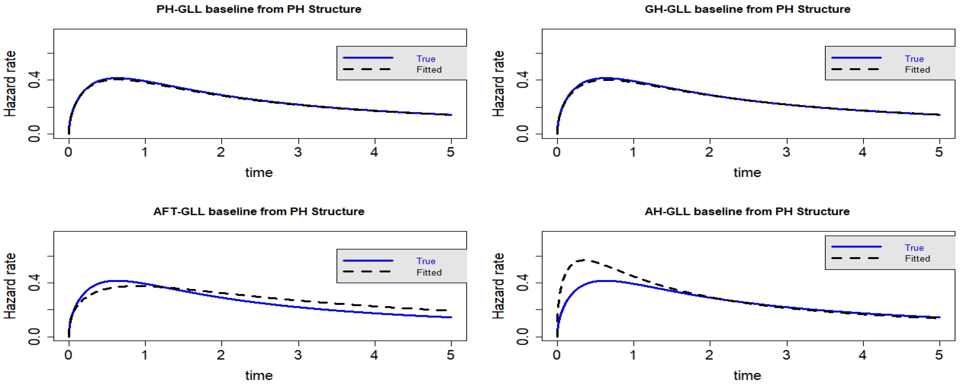
Figure 9.
Estimated baseline hrfs with censoring proportion of and a sample size of . The dashed and solid curves indicate the estimated and true hrfs, accordingly. The data generated from a PH structure.
Figure 9.
Estimated baseline hrfs with censoring proportion of and a sample size of . The dashed and solid curves indicate the estimated and true hrfs, accordingly. The data generated from a PH structure.
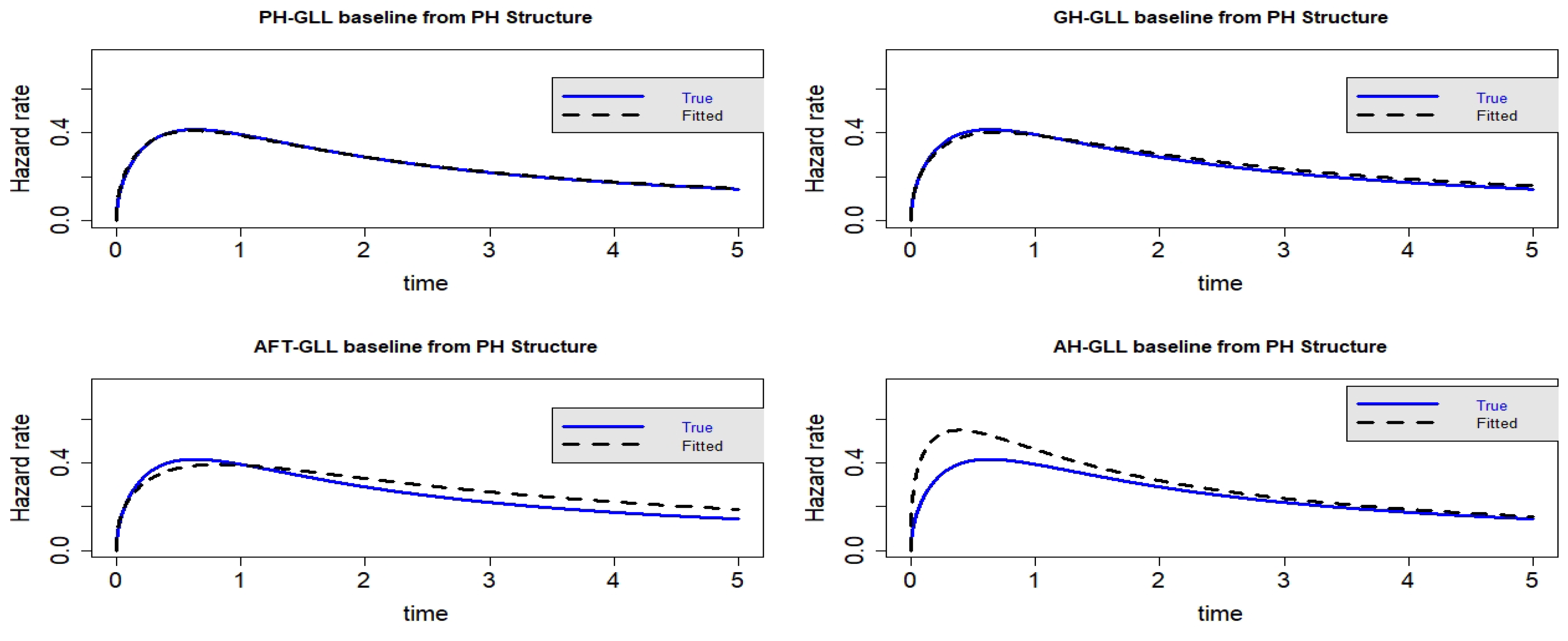
Figure 10.
Estimated baseline hrfs with censoring proportion of and a sample size of . The dashed and solid curves indicate the estimated and true hrfs, accordingly. The data generated from a PH structure.
Figure 10.
Estimated baseline hrfs with censoring proportion of and a sample size of . The dashed and solid curves indicate the estimated and true hrfs, accordingly. The data generated from a PH structure.
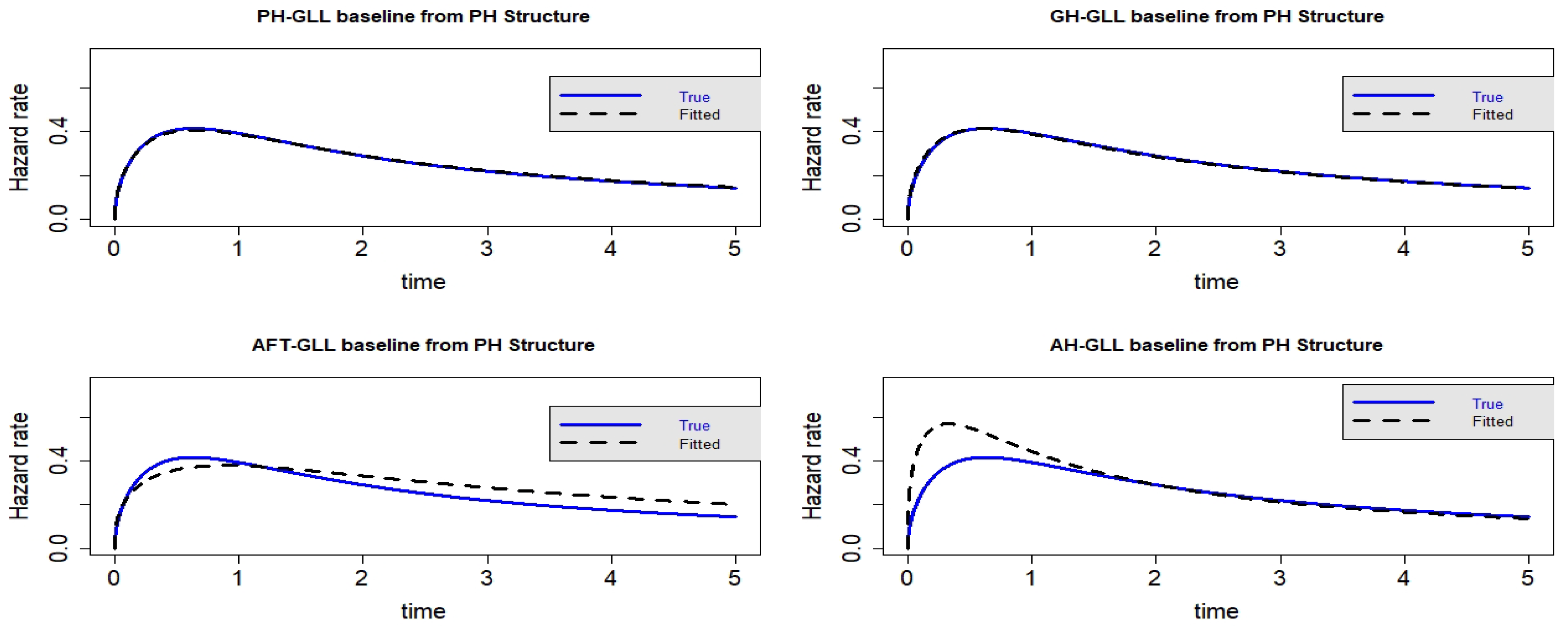
Figure 11.
Estimated baseline hrfs with censoring proportion of and a sample size of n = 10,000. The dashed and solid curves indicate the estimated and true hrfs, accordingly. The data generated from a PH structure.
Figure 11.
Estimated baseline hrfs with censoring proportion of and a sample size of n = 10,000. The dashed and solid curves indicate the estimated and true hrfs, accordingly. The data generated from a PH structure.
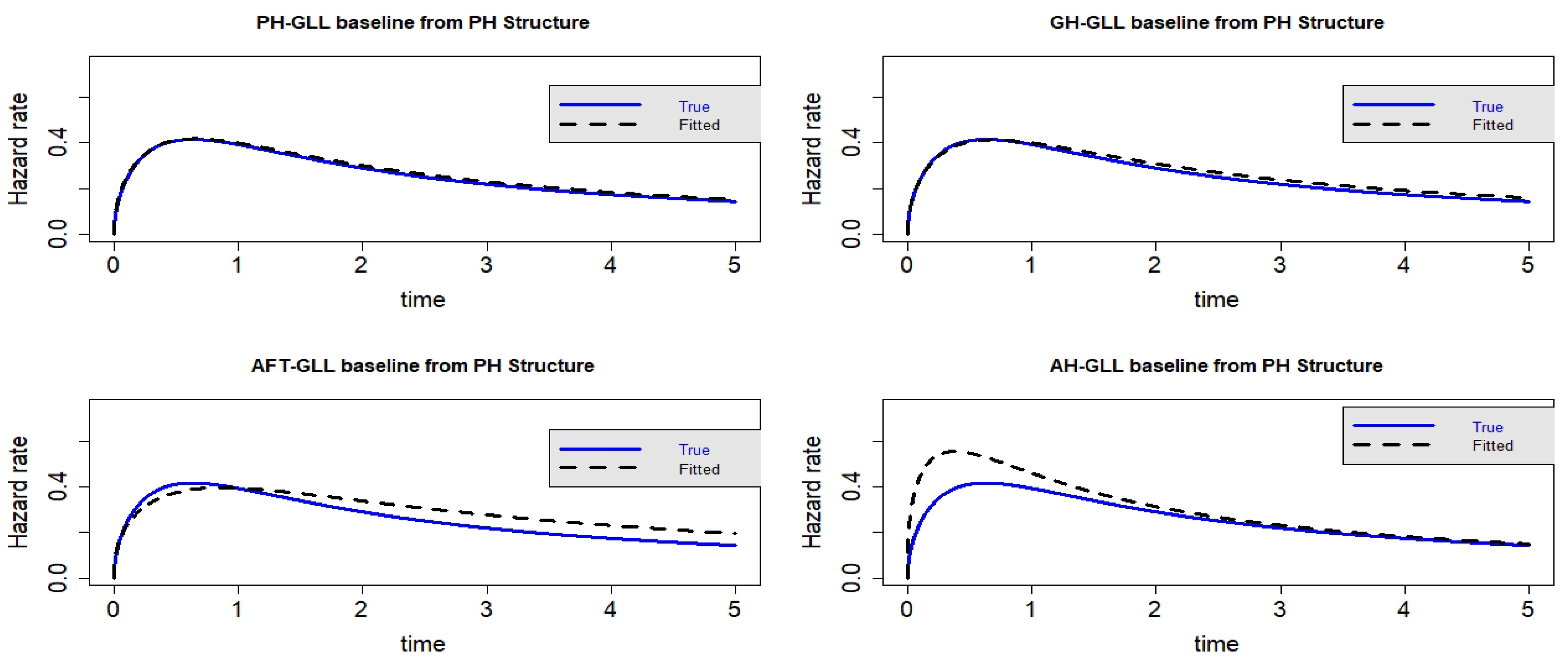
Figure 12.
Estimated baseline hrfs with censoring proportion of and a sample size of n = 10,000. The dashed and solid curves indicate the estimated and true hrfs, accordingly. The data generated from a PH structure.
Figure 12.
Estimated baseline hrfs with censoring proportion of and a sample size of n = 10,000. The dashed and solid curves indicate the estimated and true hrfs, accordingly. The data generated from a PH structure.
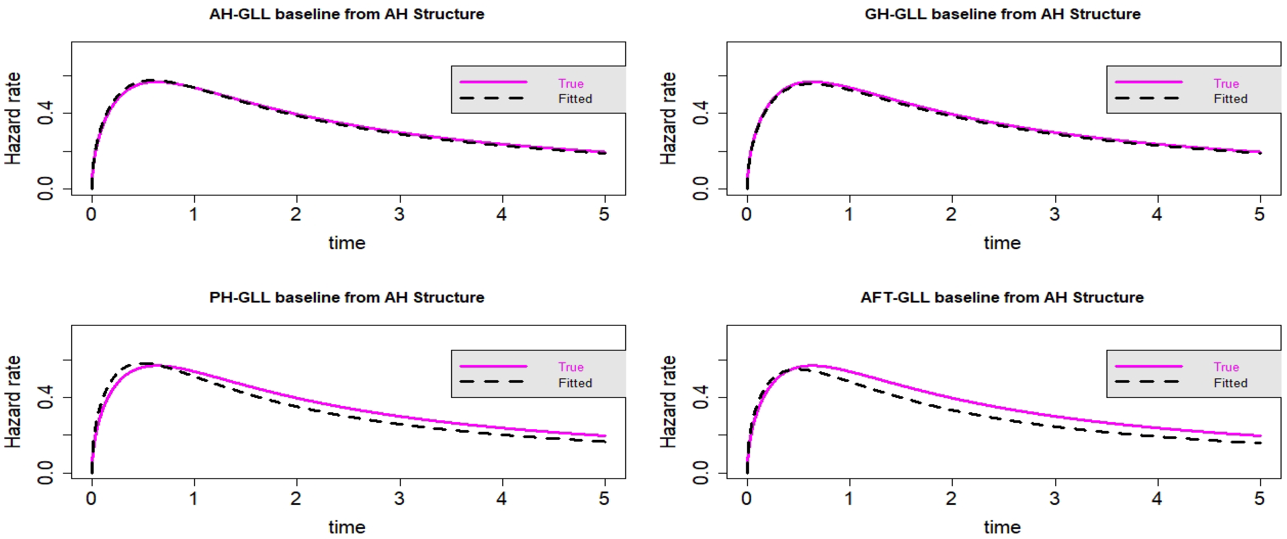
Figure 13.
Estimated baseline hrfs with censoring proportion of and a sample size of . The dashed and solid curves indicate the estimated and true hrfs, accordingly. The data generated from an AH structure.
Figure 13.
Estimated baseline hrfs with censoring proportion of and a sample size of . The dashed and solid curves indicate the estimated and true hrfs, accordingly. The data generated from an AH structure.
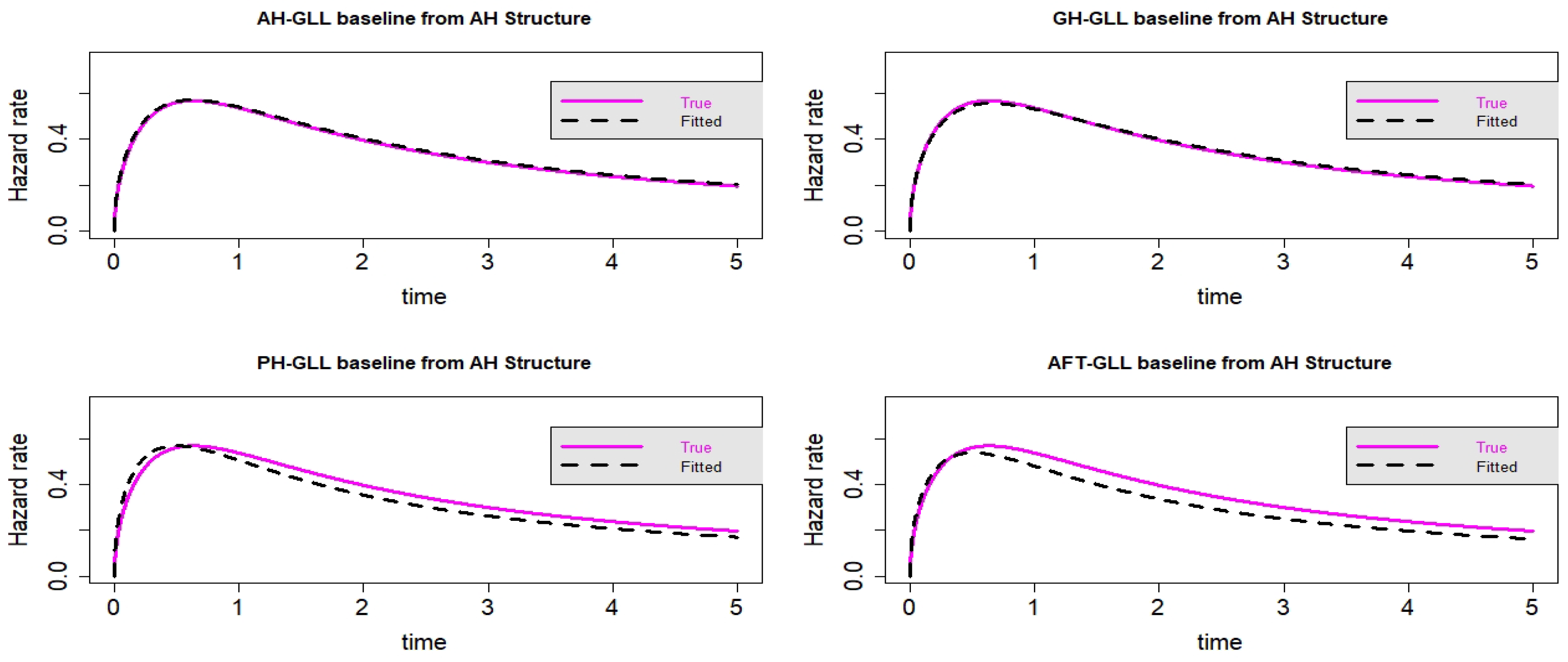
Figure 14.
Estimated baseline hrfs with censoring proportion of and a sample size of . The dashed and solid curves indicate the estimated and true hrfs, accordingly. The data generated from an AH structure.
Figure 14.
Estimated baseline hrfs with censoring proportion of and a sample size of . The dashed and solid curves indicate the estimated and true hrfs, accordingly. The data generated from an AH structure.
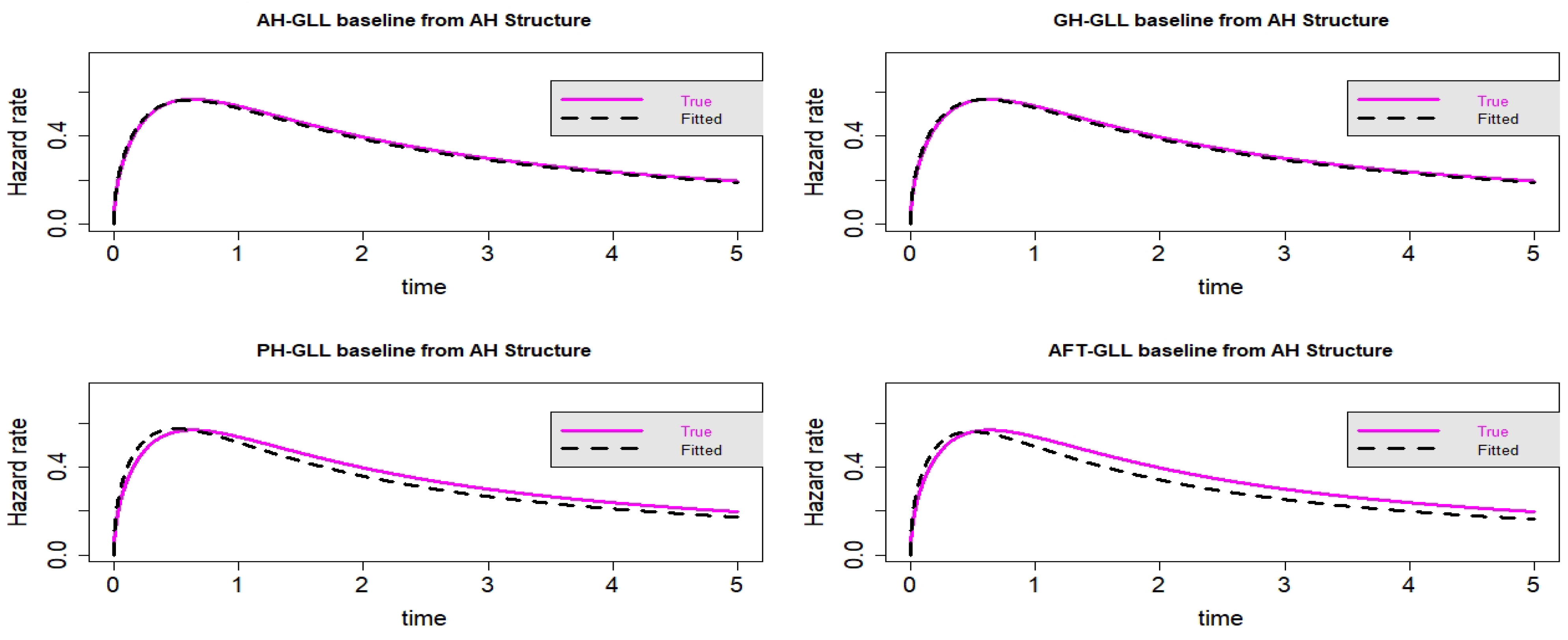
Figure 15.
Estimated baseline hrfs with censoring proportion of and a sample size of n = 10,000. The dashed and solid curves indicate the estimated and true hrfs, accordingly. The data generated from an AH structure.
Figure 15.
Estimated baseline hrfs with censoring proportion of and a sample size of n = 10,000. The dashed and solid curves indicate the estimated and true hrfs, accordingly. The data generated from an AH structure.
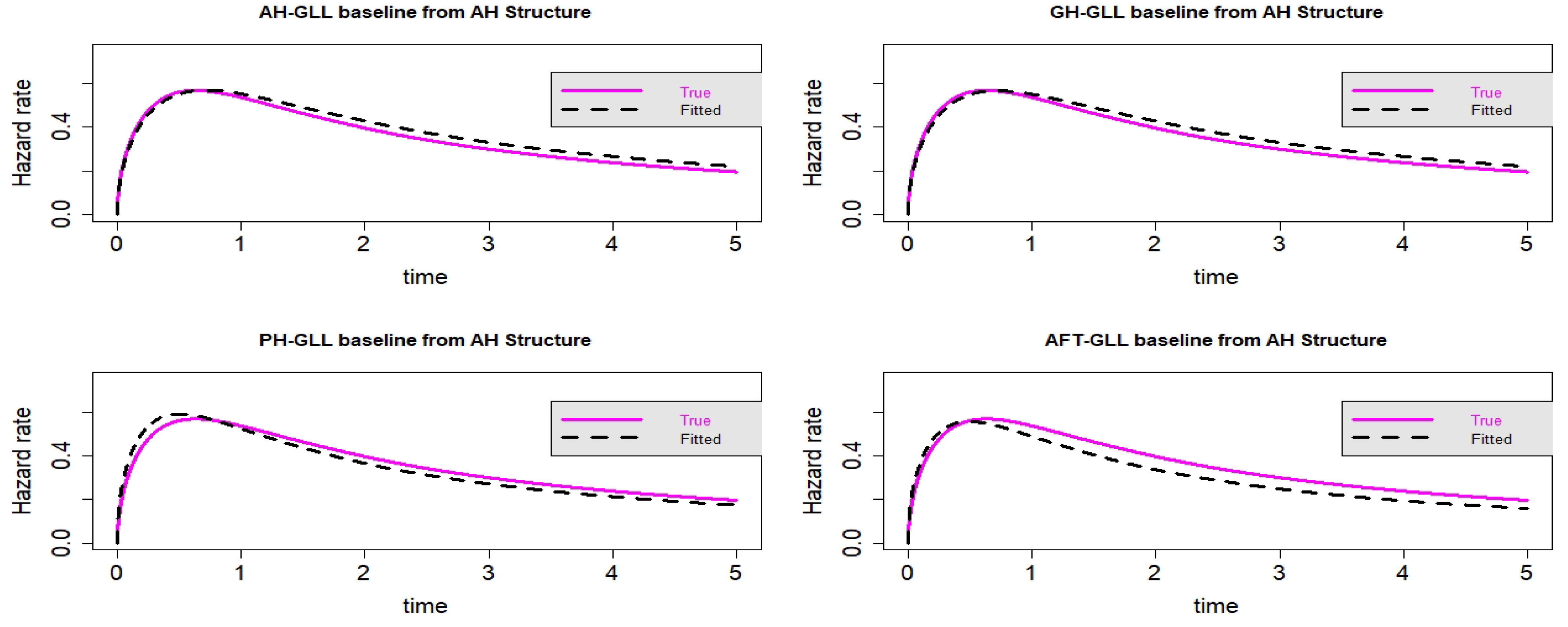
Figure 16.
Estimated baseline hrfs with censoring proportion of and a sample size of n = 10,000. The dashed and solid curves indicate the estimated and true hrfs, accordingly. The data generated from an AH structure.
Figure 16.
Estimated baseline hrfs with censoring proportion of and a sample size of n = 10,000. The dashed and solid curves indicate the estimated and true hrfs, accordingly. The data generated from an AH structure.
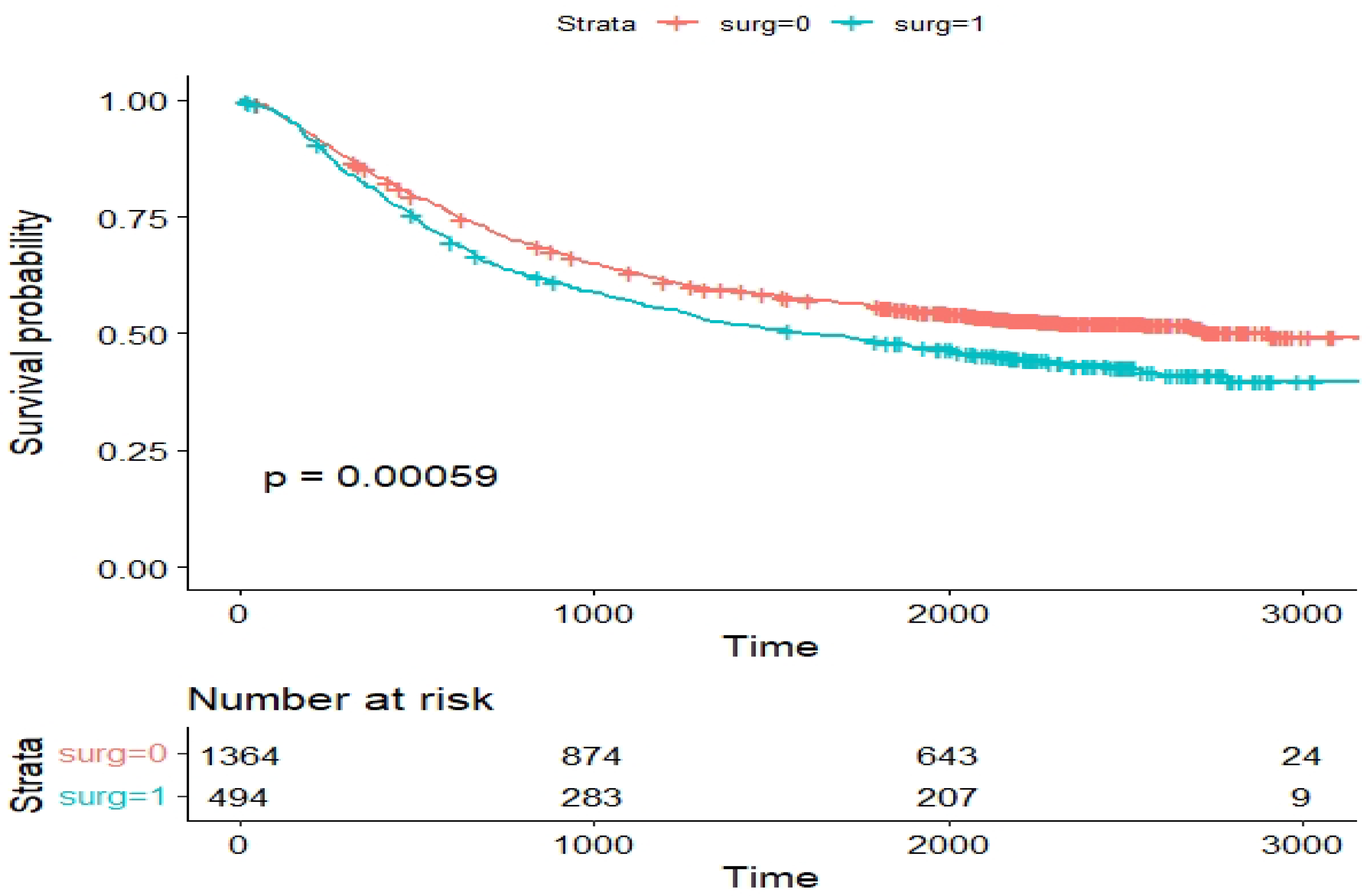
Figure 17.
Kaplan–Meier survival plot for the variable surgery status ().
Figure 17.
Kaplan–Meier survival plot for the variable surgery status ().
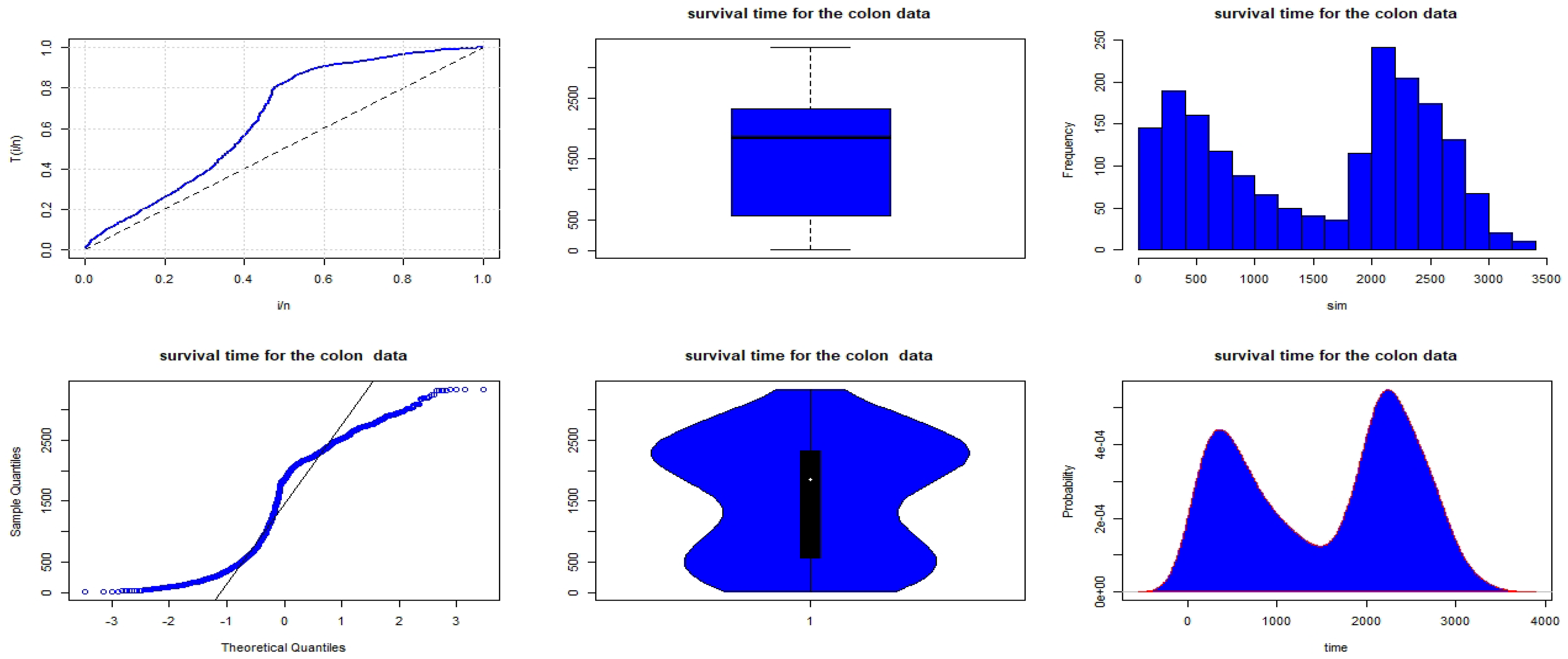
Figure 18.
Non-parametric plots for the survival time data of colon cancer patients.
Figure 18.
Non-parametric plots for the survival time data of colon cancer patients.
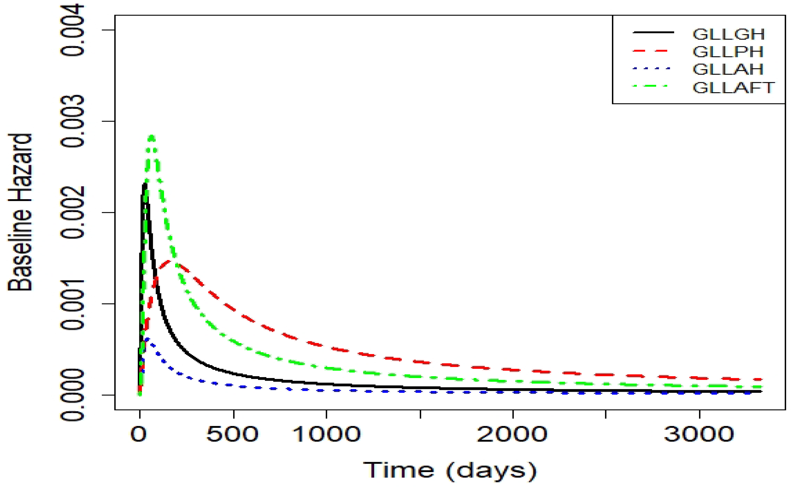
Figure 19.
Estimated hazards for the competitive models of the colon cancer dataset.
Figure 19.
Estimated hazards for the competitive models of the colon cancer dataset.
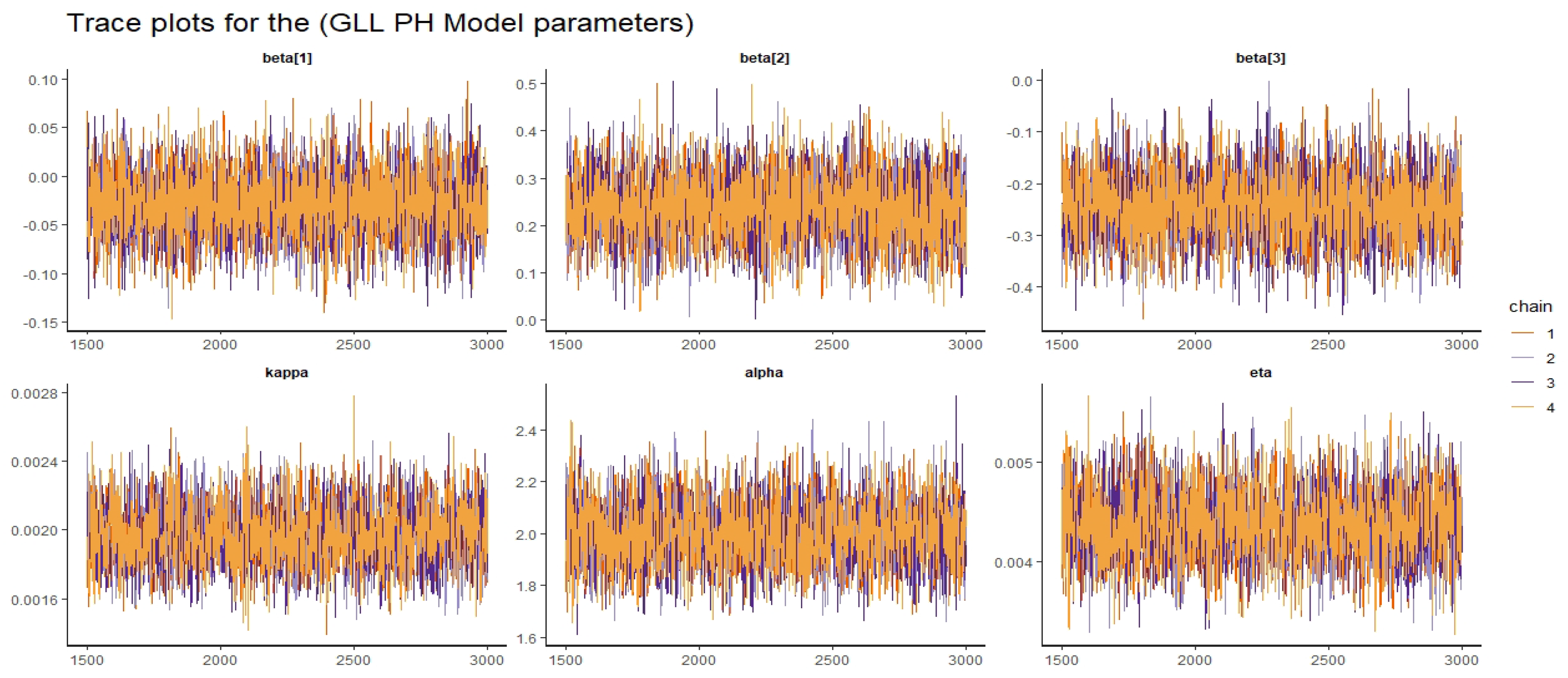
Figure 20.
Trace plots for the GLL-PH model parameters.
Figure 20.
Trace plots for the GLL-PH model parameters.
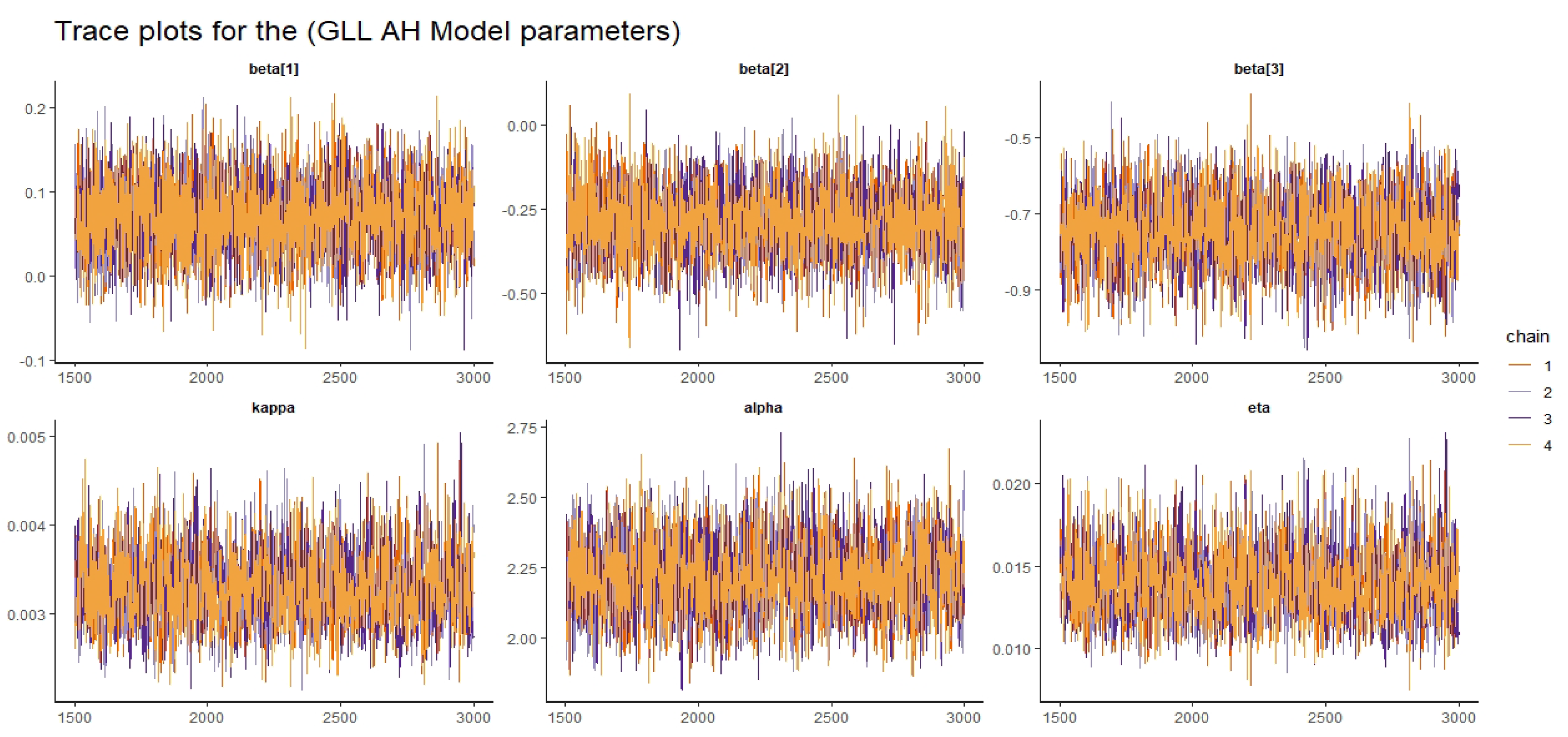
Figure 21.
Trace plots for the GLL-AH model parameters.
Figure 21.
Trace plots for the GLL-AH model parameters.
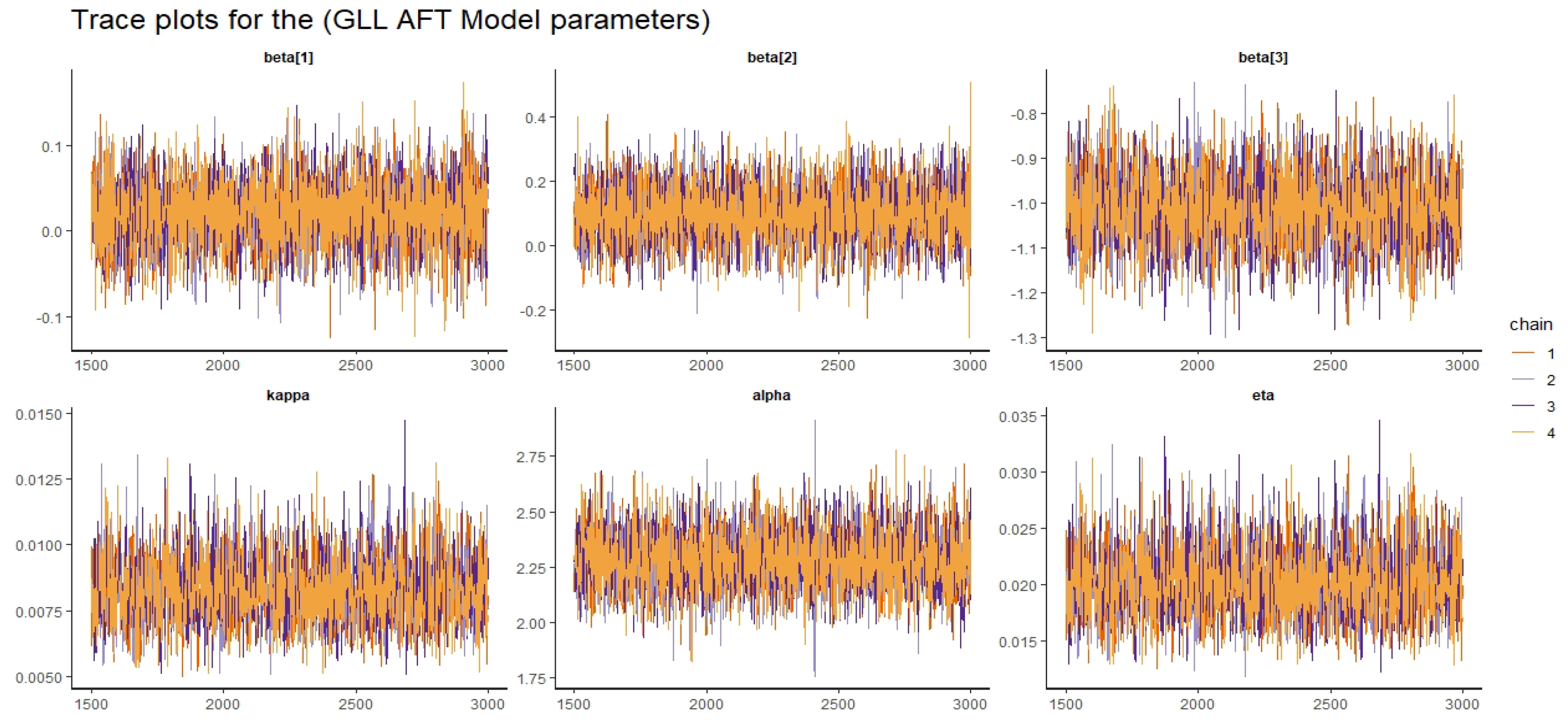
Figure 22.
Trace plots for the GLL-AFT model parameters.
Figure 22.
Trace plots for the GLL-AFT model parameters.
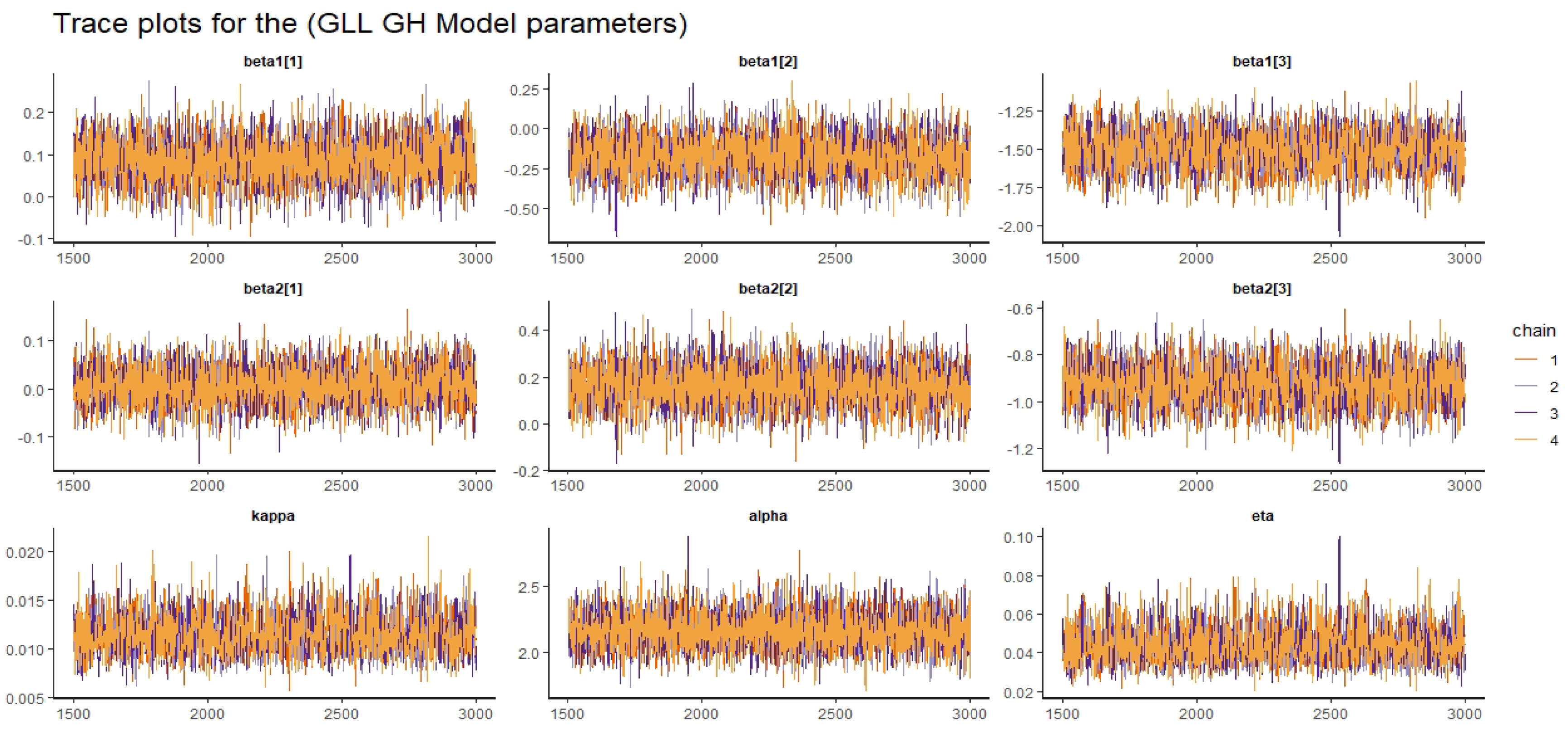
Figure 23.
Trace plots for the GLL-GH model parameters.
Figure 23.
Trace plots for the GLL-GH model parameters.
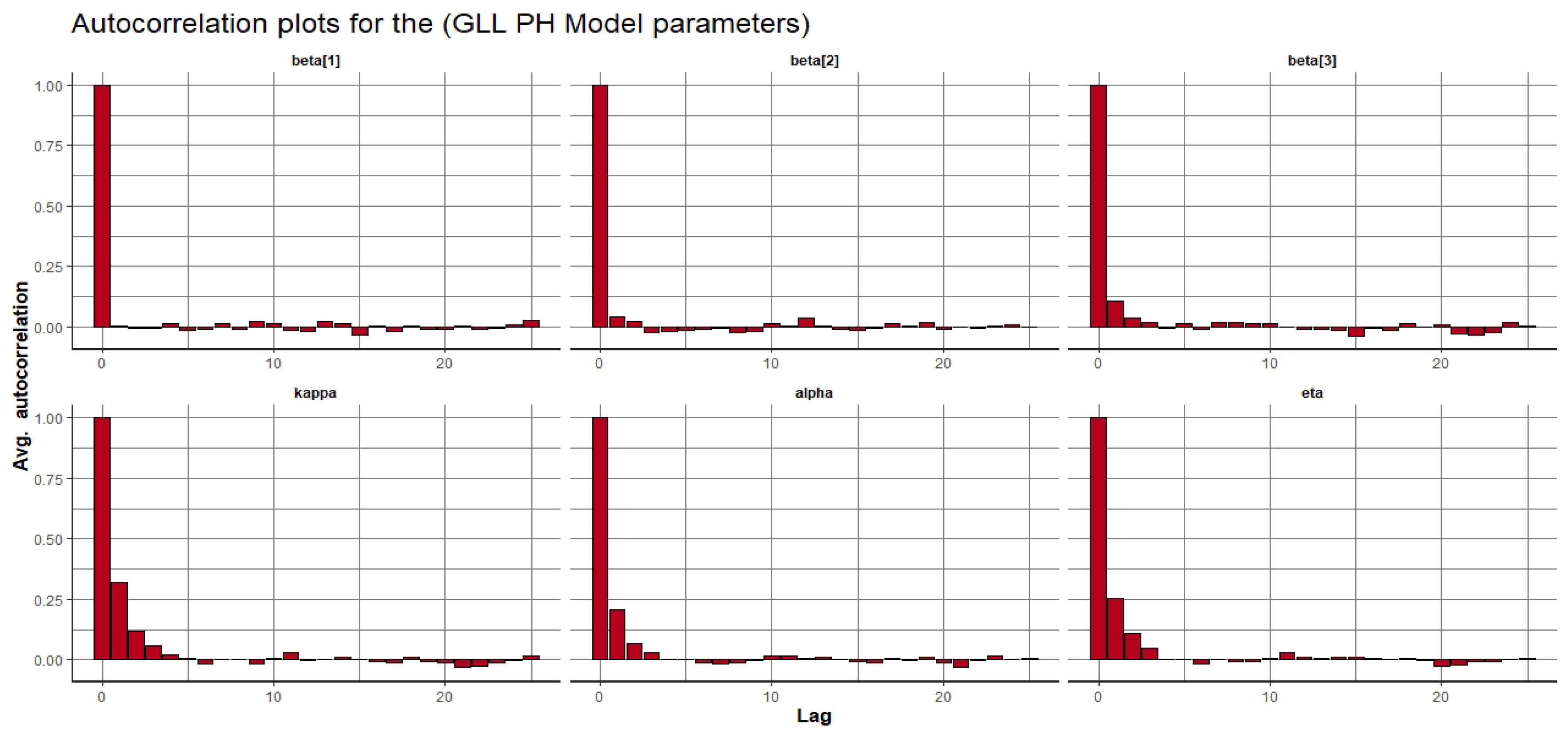
Figure 24.
Autocorrelation plots for the GLL-PH model parameters.
Figure 24.
Autocorrelation plots for the GLL-PH model parameters.
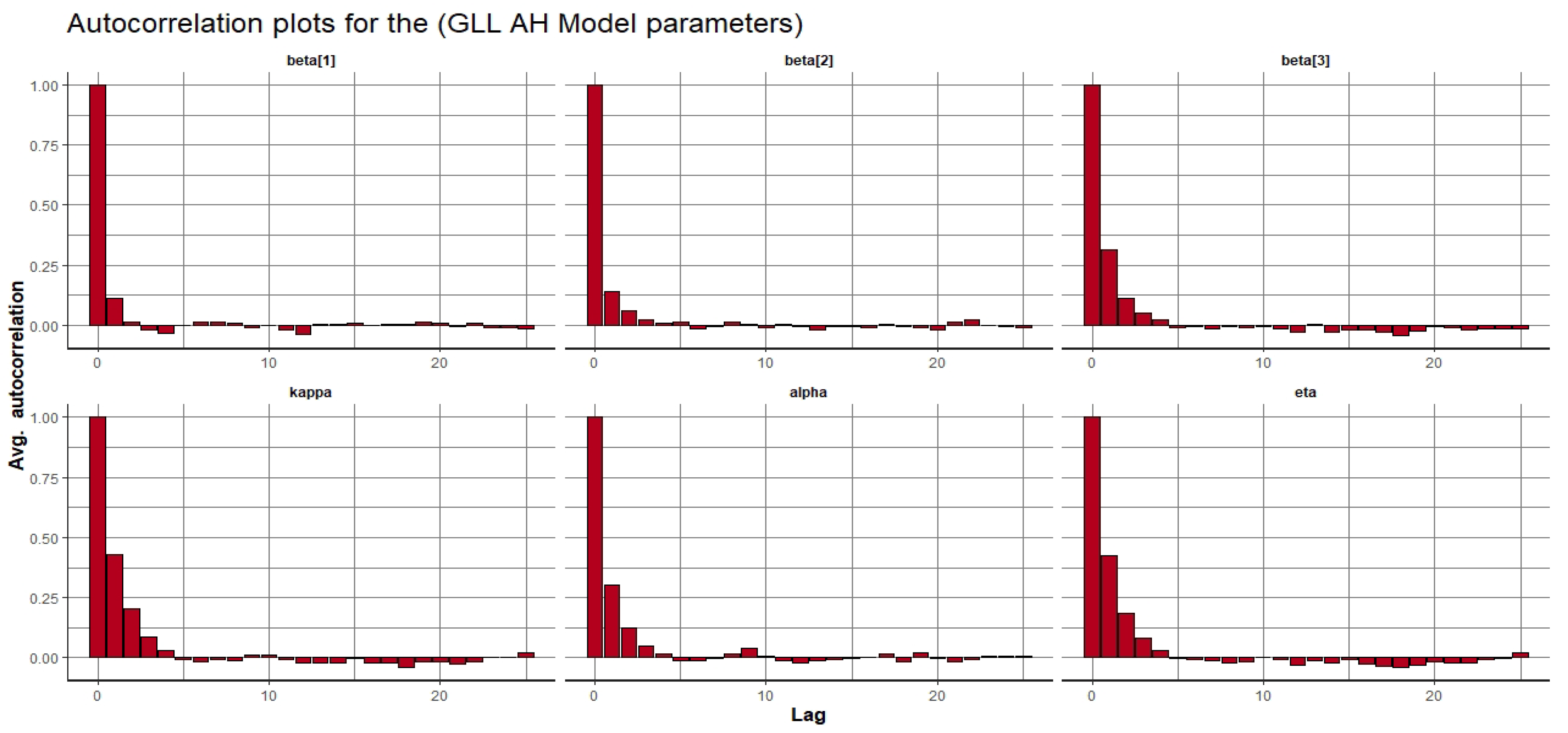
Figure 25.
Autocorrelation plots for the GLL-AH model parameters.
Figure 25.
Autocorrelation plots for the GLL-AH model parameters.
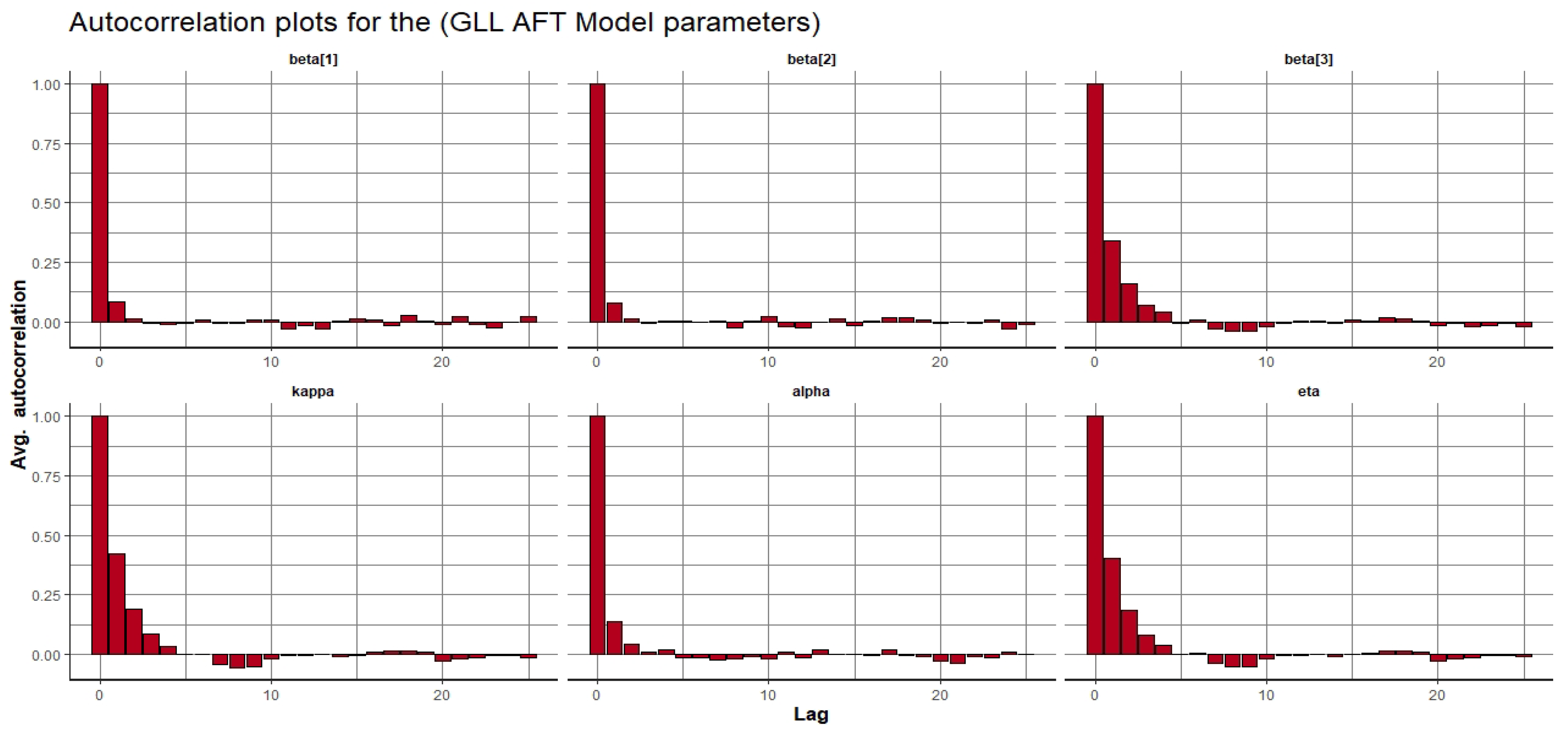
Figure 26.
Autocorrelation plots for the GLL-AFT model parameters.
Figure 26.
Autocorrelation plots for the GLL-AFT model parameters.
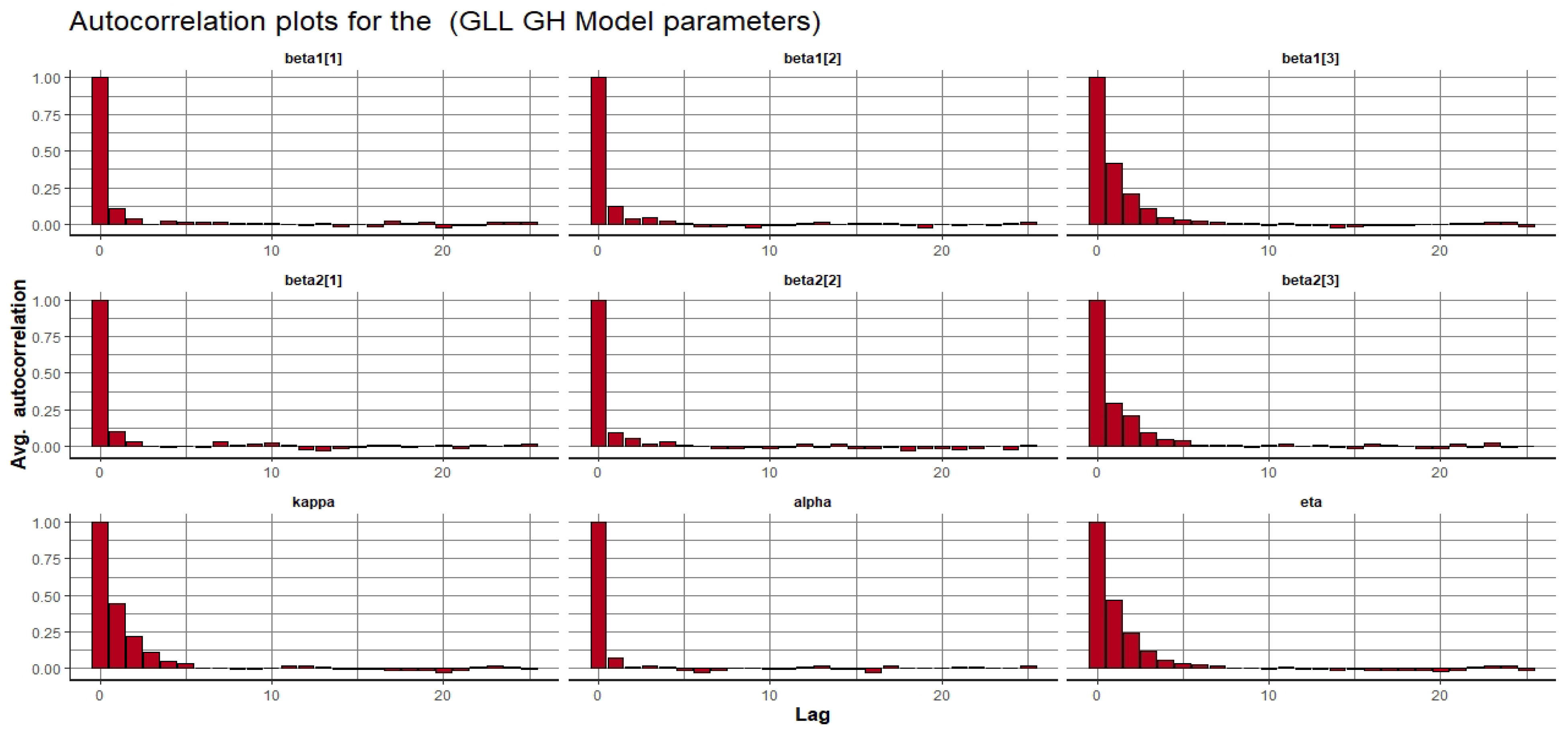
Figure 27.
Autocorrelation plots for the GLL-GH model parameters.
Figure 27.
Autocorrelation plots for the GLL-GH model parameters.
Table 1.
Summary of Parameter interpretation and comparison of PH, AH, and AFT Models.
Table 1.
Summary of Parameter interpretation and comparison of PH, AH, and AFT Models.
| | AH Model | PH Model | AFT Model |
|---|
| effect | treatment | treatment | treatment |
| | accelerates the hazard | proportionally increases | decelerates failure |
| | by a factor | hazard by a factor | time of the survivor |
| | of | of | function by a factor |
| | | | of |
| | treatment | treatment | treatment |
| | decelerates the hazard | proportionally decreases | accelerates failure |
| | by a factor | hazard by a factor | time of the survivor |
| | of | of | function by a factor |
| | | | of |
| ’s interpretation | Hazard progression | hazard ratio | Survival time |
| | time ratio | | ratio |
| limited to crossover | No | Yes | Yes |
| in hazards | | | |
| limited to crossover | No | Yes | No |
| in survival | | | |
Table 2.
Simulation results from the GH model with , and , covariates values for , ) and with about censoring. AIC, CAIC, and HQIC values for the competitive models.
Table 2.
Simulation results from the GH model with , and , covariates values for , ) and with about censoring. AIC, CAIC, and HQIC values for the competitive models.
| Model | AIC | CAIC | HQIC |
|---|
| | | % Censoring | |
| GLL-GH Model | | | |
| GLL-AFT Model | | | |
| GLL-AH Model | | | |
| GLL-PH Model | | | |
| | | % censoring | |
| GLL-GH Model | | | |
| GLL-AFT Model | | | |
| GLL-AH Model | | | |
| GLL-PH Model | | | |
Table 3.
Simulation results from the GH model with , and , covariates values for , ) and n = 10,000 with about censoring. AIC, CAIC, and HQIC values for the competitive models.
Table 3.
Simulation results from the GH model with , and , covariates values for , ) and n = 10,000 with about censoring. AIC, CAIC, and HQIC values for the competitive models.
| Model | AIC | CAIC | HQIC |
|---|
| | | % Censoring | |
| GLL-GH Model | 17,567.525 | 175,672 | 17,589.491 |
| GLL-AFT Model | 17,843.352 | 17,843.429 | 17,857.996 |
| GLL-AH Model | 24,035.240 | 24,035.198 | 24,049.884 |
| GLL-PH Model | 17,818.738 | 17,818.184 | 17,833.382 |
| | | % censoring | |
| GLL-GH Model | 10,719.862 | 10,719.901 | 10,741.828 |
| GLL-AFT Model | 10,809.107 | 10,809.125 | 10,823.751 |
| GLL-AH Model | 14,662.298 | 14,662.330 | 14,676.942 |
| GLL-PH Model | 10,913.655 | 10,913.673 | 10,928.299 |
Table 4.
Simulation results from the AFT model with , and , covariates values for , and with about and censoring. AIC, CAIC, and HQIC values for the competitive models.
Table 4.
Simulation results from the AFT model with , and , covariates values for , and with about and censoring. AIC, CAIC, and HQIC values for the competitive models.
| | AIC | CAIC | HQIC |
|---|
| | | % Censoring | |
| GLL-AFT Model | 9710.030 | 9710.583 | 9723.735 |
| GLL-GH Model | 9713.632 | 9714.807 | 9734.190 |
| GLL-AH Model | 12,766.930 | 12,766.869 | 12,780.635 |
| GLL-PH Model | 10,241.712 | 10,240.974 | 10,255.417 |
| | | Censoring | |
| GLL-AFT Model | 6119.325 | 6119.367 | 6133.030 |
| GLL-GH Model | 6122.154 | 6122.246 | 6142.711 |
| GLL-PH Model | 6500.689 | 6500.739 | 6514.394 |
| GLL-AH Model | 8259.059 | 8249.154 | 8262.764 |
Table 5.
Simulation results from the AFT model with , and , covariates values for , and n = 10,000 with about and censoring. AIC, CAIC, and HQIC values for the competitive models.
Table 5.
Simulation results from the AFT model with , and , covariates values for , and n = 10,000 with about and censoring. AIC, CAIC, and HQIC values for the competitive models.
| Model | AIC | CAIC | HQIC |
|---|
| | | % Censoring | |
| GLL-AFT Model | 19,192.366 | 19,192.571 | 19,207.011 |
| GLL-GH Model | 19,195.876 | 19,196.313 | 19,217.842 |
| GLL-AH Model | 25,043.290 | 12,766.257 | 25,057.934 |
| GLL-PH Model | 20,201.167 | 20,200.269 | 20,215.811 |
| | | censoring | |
| GLL-AFT Model | 12,214.303 | 12,214.324 | 12,228.947 |
| GLL-GH Model | 12,211.367 | 12,211.413 | 12,233.332 |
| GLL-PH Model | 13,036.386 | 13,036.410 | 13,051.030 |
| GLL-AH Model | 16,233.077 | 16,233.122 | 16,247.721 |
Table 6.
Simulation results from the PH model with , and , covariates values for , and with about and censoring. AIC, CAIC, and HQIC values for the competitive models.
Table 6.
Simulation results from the PH model with , and , covariates values for , and with about and censoring. AIC, CAIC, and HQIC values for the competitive models.
| Model | AIC | CAIC | HQIC |
|---|
| | | % Censoring | |
| GLL-PH Model | 14,941.383 | 14,941.349 | 14,955.088 |
| GLL-GH Model | 14,947.070 | 14,946.997 | 14,967.627 |
| GLL-AFT Model | 15,037.394 | 15,037.361 | 15,051.100 |
| GLL-AH Model | 15,224.134 | 15,224.102 | 15,237.840 |
| | | Censoring
| |
| GLL-PH Model | 10,966.406 | 10,966.229 | 10,980.111 |
| GLL-GH Model | 10,966.497 | 10,966.116 | 10,987.054 |
| GLL-AFT Model | 11,038.579 | 11,038.415 | 11,052.284 |
| GLL-AH Model | 11,206.019 | 11,205.877 | 11,219.724 |
Table 7.
Simulation results from the PH model with , and , covariates values for , and with about and censoring. AIC, CAIC, and HQIC values for the competitive models.
Table 7.
Simulation results from the PH model with , and , covariates values for , and with about and censoring. AIC, CAIC, and HQIC values for the competitive models.
| Model | AIC | CAIC | BIC |
|---|
| | | % Censoring | |
| GLL-PH Model | 29,768.943 | 29,768.927 | 29,783.588 |
| GLL-GH Model | 29,772.045 | 29,772.008 | 29,794.011 |
| GLL-AFT Model | 29,969.703 | 29,969.686 | 29,984.345 |
| GLL-AH Model | 30,321.478 | 30,321.462 | 30,336.123 |
| | | Censoring | |
| GLL-PH Model | 22,085.485 | 22,085.404 | 22,100.129 |
| GLL-GH Model | 22,088.317 | 22,088.143 | 22,110.283 |
| GLL-AFT Model | 22,219.687 | 22,219.611 | 22,234.331 |
| GLL-AH Model | 22,560.893 | 22,560.828 | 22,575.538 |
Table 8.
Simulation results from the AH model with , and , covariates values for , and with about and censoring. AIC, CAIC, and HQIC values for the competitive models.
Table 8.
Simulation results from the AH model with , and , covariates values for , and with about and censoring. AIC, CAIC, and HQIC values for the competitive models.
| Model | AIC | CAIC | HQIC |
|---|
| | | % Censoring | |
| GLL-AH Model | 15,084.818 | 15,084.785 | 15,098.523 |
| GLL-GH Model | 15,086.243 | 15,086.172 | 15,106.801 |
| GLL-PH Model | 15,161.428 | 15,161.396 | 15,175.133 |
| GLL-AFT Model | 15,212.691 | 15,212.658 | 15,226.396 |
| | | % Censoring | |
| GLL-AH Model | 11,154.225 | 11,154.078 | 11,167.930 |
| GLL-GH Model | 11,156.478 | 11,156.161 | 11,177.035 |
| GLL-PH Model | 11,229.268 | 11,229.130 | 11,242.974 |
| GLL-AFT Model | 11,252.678 | 11,252.542 | 11,266.382 |
Table 9.
Simulation results from the AH model with , and , covariates values for , and with about and censoring. AIC, CAIC, and HQIC values for the competitive models.
Table 9.
Simulation results from the AH model with , and , covariates values for , and with about and censoring. AIC, CAIC, and HQIC values for the competitive models.
| Model | AIC | CAIC | HQIC |
|---|
| | | % Censoring | |
| GLL-AFT Model | 30,458.953 | 30,458.937 | 30,473.597 |
| GLL-GH Model | 30,463.451 | 30,463.416 | 30,485.416 |
| GLL-AH Model | 30,664.667 | 30,664.651 | 30,679.310 |
| GLL-PH Model | 30,741.659 | 30,741.644 | 30,756.303 |
| | | Censoring | |
| GLL-AFT Model | 22,592.371 | 22,592.306 | 22,607.015 |
| GLL-AFT Model | 22,598.029 | 22,597.890 | 22,619.996 |
| GLL-GH Model | 22,776.538 | 22,776.477 | 22,791.182 |
| GLL-AH Model | 22,822.921 | 22,822.861 | 22,837.565 |
Table 10.
Results of the McMC simulation for Study II (Bayesian inference) under the GLL-GH framework with baseline hazard parameter values of , and ; covariate values of ; sample size of 100; and two censoring proportions for rates of 20 and .
Table 10.
Results of the McMC simulation for Study II (Bayesian inference) under the GLL-GH framework with baseline hazard parameter values of , and ; covariate values of ; sample size of 100; and two censoring proportions for rates of 20 and .
| True Value | Posterior Mean | AB | MSE | CP | n-eff | |
|---|
| | | | 20% Censoring | | | |
| 0.260 | 0.010 | 0.005 | 94.13 | 5232 | 1.002 |
| 0.378 | 0.028 | 0.014 | 93.96 | 4313 | 1.002 |
| 0.475 | 0.025 | 0.010 | 94.60 | 4717 | 1.000 |
| 0.595 | 0.045 | 0.015 | 93.88 | 3987 | 1.000 |
| 0.714 | 0.064 | 0.026 | 92.37 | 3243 | 1.000 |
| 0.822 | 0.072 | 0.032 | 95.03 | 3456 | 1.000 |
| 1.425 | 0.025 | 0.011 | 94.50 | 5404 | 1.001 |
| 0.833 | 0.033 | 0.025 | 94.23 | 5039 | 1.002 |
| 1.224 | 0.024 | 0.021 | 95.67 | 4788 | 1.002 |
| | | | 30% Censoring | | | |
| 0.292 | 0.042 | 0.007 | 92.47 | 5032 | 1.003 |
| 0.386 | 0.036 | 0.015 | 92.55 | 4519 | 1.004 |
| 0.483 | 0.033 | 0.012 | 93.41 | 4788 | 1.001 |
| 0.606 | 0.056 | 0.018 | 94.69 | 3987 | 1.001 |
| 0.720 | 0.070 | 0.023 | 96.82 | 3832 | 1.001 |
| 0.831 | 0.081 | 0.033 | 94.45 | 4156 | 1.000 |
| 1.436 | 0.036 | 0.013 | 96.32 | 5122 | 1.002 |
| 0.847 | 0.047 | 0.028 | 91.60 | 5039 | 1.001 |
| 1.232 | 0.032 | 0.024 | 93.09 | 5188 | 1.001 |
Table 11.
Results of the McMC simulation for Study II (Bayesian inference) under the GLL-GH framework with baseline hazard parameter values of , and ; covariate values of ; sample size of 300; and two censoring proportions for rates of 20 and .
Table 11.
Results of the McMC simulation for Study II (Bayesian inference) under the GLL-GH framework with baseline hazard parameter values of , and ; covariate values of ; sample size of 300; and two censoring proportions for rates of 20 and .
| True Value | Posterior Mean | AB | MSE | CP | n-eff | |
|---|
| | | | 20% Censoring | | | |
| 0.258 | 0.008 | 0.004 | 95.14 | 4898 | 1.000 |
| 0.368 | 0.018 | 0.012 | 95.03 | 4020 | 1.000 |
| 0.470 | 0.020 | 0.008 | 94.93 | 5676 | 1.000 |
| 0.590 | 0.040 | 0.013 | 95.80 | 5413 | 1.000 |
| 0.704 | 0.054 | 0.024 | 94.80 | 5213 | 1.000 |
| 0.802 | 0.052 | 0.030 | 95.04 | 5093 | 1.000 |
| 1.425 | 0.025 | 0.010 | 95.12 | 5003 | 1.000 |
| 0.803 | 0.003 | 0.002 | 95.07 | 4937 | 1.000 |
| 1.204 | 0.004 | 0.003 | 94.92 | 4953 | 1.000 |
| | | | 30% Censoring | | | |
| 0.292 | 0.042 | 0.006 | 94.00 | 5099 | 1.000 |
| 0.386 | 0.036 | 0.014 | 95.25 | 5676 | 1.001 |
| 0.483 | 0.033 | 0.011 | 94.763 | 55122 | 1.000 |
| 0.606 | 0.321 | 0.013 | 95.43 | 3056 | 1.002 |
| 0.720 | 0.70 | 0.020 | 95.55 | 3898 | 1.001 |
| 0.831 | 0.081 | 0.031 | 94.34 | 4454 | 1.000 |
| 1.436 | 0.036 | 0.012 | 96.32 | 4989 | 1.001 |
| 0.847 | 0.047 | 0.026 | 95.00 | 5006 | 1.000 |
| 1.232 | 0.032 | 0.020 | 96.05 | 5012 | 1.001 |
Table 12.
Results from the fitted parametric hazard-based regression models to colon cancer dataset.
Table 12.
Results from the fitted parametric hazard-based regression models to colon cancer dataset.
| Models | Parameter(s) | Estimate | SE | Z-Value | p-Value | L-95% | U-95% |
|---|
| GLL-GH | | 0.065 | 0.038 | 0.593 | 0.553 | −0.053 | 0.171 |
| | | −0.171 | 0.129 | −1.331 | 0.183 | −0.423 | 0.081 |
| | | −1.549 | 0.118 | −13.185 | <0.001 | −1.780 | −1.139 |
| | | 0.012 | 0.039 | 0.316 | 0.752 | −0.065 | 0.090 |
| | | 0.161 | 0.087 | 1.850 | 0.064 | −0.010 | 0.331 |
| | | −0.890 | 0.072 | −12.339 | <0.001 | −1.032 | −0.749 |
| | | 1.938 | 0.127 | 8.932 | <0.001 | 1.690 | 2.187 |
| | | 0.009 | 0.001 | 15.290 | <0.001 | 0.007 | 0.011 |
| | | 0.039 | 0.006 | 6.697 | <0.001 | 0.028 | 0.187 |
| GLL-AFT | | 0.023 | 0.038 | 0.593 | 0.553 | −0.053 | 0.098 |
| | | 0.100 | 0.089 | 1.131 | 0.258 | −0.074 | 0.274 |
| | | −0.970 | 0.058 | −16.864 | <0.001 | −1.083 | −0.857 |
| | | 2.381 | 0.139 | 17.175 | <0.001 | 2.161 | 2.653 |
| | | 0.008 | 0.001 | 10.986 | <0.001 | 0.011 | 0.009 |
| | | 0.019 | 0.002 | 11.213 | <0.001 | 0.042 | 0.022 |
| GLL-PH | | −0.064 | 0.033 | −1.936 | 0.043 | −0.129 | 0.001 |
| | | 0.167 | 0.072 | 2.323 | 0.020 | 0.026 | 0.309 |
| | | −0.518 | 0.052 | −9.978 | <0.001 | −0.620 | −0.417 |
| | | 1.938 | 0.127 | 8.932 | <0.001 | 1.690 | 2.187 |
| | | 0.009 | 0.001 | 15.290 | <0.001 | 0.007 | 0.011 |
| | | 0.039 | 0.006 | 6.697 | <0.001 | 0.028 | 0.187 |
| GLL-AH | | 0.029 | 0.047 | 0.620 | 0.535 | −0.062 | 0.120 |
| | | −0.464 | 0.108 | −4.288 | <0.001 | −0.676 | −0.252 |
| | | −1.139 | 0.090 | −12.648 | <0.001 | −1.315 | −0.962 |
| | | 2.113 | 0.084 | 25.226 | <0.001 | 2.161 | 2.277 |
| | | 0.004 | 0.000 | 17.158 | <0.001 | 0.011 | 0.005 |
| | | 0.024 | 0.003 | 9.495 | <0.001 | 0.042 | 0.029 |
Table 13.
Results for some frequentist information criteria for the hazard-based regression models.
Table 13.
Results for some frequentist information criteria for the hazard-based regression models.
| Model | AIC | CAIC | HQIC |
|---|
| GH | 16,276.09 | 16,276.07 | 16,294.43 |
| PH | 16,415.50 | 16,415.50 | 16,427.74 |
| AH | 16,384.96 | 16,384.94 | 16,397.94 |
| AFT | 16,294.36 | 16,294.35 | 16,306.58 |
Table 14.
LRT test for the GH model and its sub-models.
Table 14.
LRT test for the GH model and its sub-models.
| Model | Hypothesis | LRT | p-Value |
|---|
| GH vs. PH | is false, | 145.424 | <0.001 |
| GH vs. AH | is false, | 114.863 | <0.001 |
| GH vs. AFT | is false, | 24.268 | <0.001 |
Table 15.
Results for the posterior properties of the competitive models.
Table 15.
Results for the posterior properties of the competitive models.
| Models | Par (s) | Estimate | SE | SD | 2.5% | Medium | 97.5% | | |
|---|
| GLL-GH | | 0.086 | 0.001 | 0. | −0.016 | 0.087 | 0.187 | 4013 | 1.001 |
| | | −0.172 | 0.002 | 0.122 | −0.412 | −0.174 | 0.067 | 4049 | 1.001 |
| | | −1.500 | 0.003 | 0.129 | −1.752 | −1.497 | −1.264 | 2174 | 1.004 |
| | | 0.009 | 0.001 | 0.040 | −0.070 | 0.009 | 0.086 | 4772 | 1.000 |
| | | 0.161 | 0.001 | 0.087 | −0.004 | 0.158 | 0.333 | 4151 | 1.001 |
| | | −0.925 | 0.002 | 0.088 | −1.097 | −0.925 | −0.756 | 2410 | 1.003 |
| | | 2.166 | 0.002 | 0.138 | 1.909 | 2.161 | 2.449 | 4951 | 1.001 |
| | | 0.011 | 0.000 | 0.002 | 0.008 | 0.011 | 0.016 | 2174 | 1.004 |
| | | 0.044 | 0.000 | 0.009 | 0.029 | 0.042 | 0.064 | 2016 | 1.004 |
| GLL-AFT | | 0.021 | 0.001 | 0.038 | −0.057 | 0.021 | 0.095 | 5059 | 1.001 |
| | | 0.101 | 0.001 | 0.089 | −0.073 | 0.100 | 0.271 | 5069 | 1.000 |
| | | −1.012 | 0.002 | 0.081 | −1.168 | −1.012 | −0.855 | 2685 | 1.001 |
| | | 2.282 | 0.002 | 0.134 | 2.033 | 2.277 | 2.554 | 4304 | 1.000 |
| | | 0.008 | 0.000 | 0.001 | 0.006 | 0.008 | 0.011 | 2426 | 1.001 |
| | | 0.020 | 0.000 | 0.003 | 0.015 | 0.020 | 0.027 | 2470 | 1.001 |
| GLL-PH | | −0.029 | 0.000 | 0.034 | −0.096 | −0.029 | 0.039 | 5944 | 1.000 |
| | | 0.238 | 0.001 | 0.071 | 0.099 | 0.238 | 0.374 | 5490 | 1.000 |
| | | −0.245 | 0.001 | 0.066 | −0.374 | −0.245 | −0.116 | 4336 | 1.000 |
| | | 1.997 | 0.002 | 0.000 | −1.767 | 1.993 | 2.242 | 3623 | 1.001 |
| | | 0.002 | 0.000 | 0.122 | 0.002 | 0.002 | 0.002 | 2912 | 1.002 |
| | | 0.004 | 0.000 | 0.000 | 0.004 | 0.004 | 0.005 | 3235 | 1.001 |
| GLL-AH | | 0.071 | 0.001 | 0.043 | −0.013 | 0.072 | 0.157 | 5046 | 1.000 |
| | | −0.283 | 0.001 | 0.098 | −0.479 | −0.282 | −0.094 | 4320 | 1.000 |
| | | −0.744 | 0.002 | 0.096 | −0.932 | −0.744 | −0.554 | 3425 | 1.001 |
| | | 2.218 | 0.002 | 0.132 | 1.970 | 2.216 | 2.487 | 3258 | 1.000 |
| | | 0.003 | 0.000 | 0.000 | 0.003 | 0.003 | 0.004 | 2728 | 1.001 |
| | | 0.014 | 0.000 | 0.002 | 0.010 | 0.014 | 0.018 | 2904 | 1.001 |
Table 16.
Bayesian model comparison for the GLL-GH and its special cases.
Table 16.
Bayesian model comparison for the GLL-GH and its special cases.
| Model | WAIC | LOOIC |
|---|
| GH | 16,274.00 | 16,274.01 |
| PH | 16,360.20 | 16,360.21 |
| AH | 16,345.80 | 16,345.90 |
| AFT | 16,295.75 | 16,295.80 |


 ,
, 


