1. Introduction
Attribute charts have important applications. They are particularly useful in service industries and in nonmanufacturing quality-improvement efforts, because so many of the quality characteristics found in these environments are not easily measured on a numerical scale [
1]. Here, we study a control chart for monitoring the number of nonconforming items. The traditional Shewhart np control charts are the statistical control scheme most commonly used for monitoring the number of nonconforming items [
1].
In a traditional Shewhart np control chart, a sample of size is taken and inspected, and the number of nonconforming items, usually denoted by , is counted. If , where is the lower control limit and is the upper control limit, the process is denoted to be in-control; otherwise, the process is assumed to be out-of-control, and corrective action should be taken.
Some research has proposed improvements to the traditional Shewhart np control chart in terms of
and
. References [
2,
3] proposed a double sampling control chart for small fraction defectives in-control (
), while [
4] designed an economic method of an attribute control chart. In [
5] an algorithm is presented for optimizing the design of the np control chart with curtailment. Reference [
6] proposed a double inspection, where the first inspection decides the process status according to the number of nonconforming units found in a sample, and the second inspection makes a decision based on the location of a particular nonconforming unit in the sample.
In [
7], a new control chart for attributes was proposed based on two different previously proposed control charts one using repetitive sampling (RS) [
8] and another one using multiple dependent state sampling (MDS) [
9]. The control chart proposed by [
7] joins these two control charts and it uses a multiple dependent state with repetitive sampling (MDSRS) which is more efficient in terms of
compared with MDS and repetitive sampling. Given the above and the topic or said paper, we will present a comparison between the proposed control chart in this work and the MDSRS control chart in
Section 3.
In other papers such as [
10,
11,
12,
13,
14,
15,
16,
17,
18,
19], more proposals for improving the np control chart can be found.
The new proposal in this article, named triple sampling np, or TS-np, consists of applying a triple sampling in every subgroup instead of taking a single sample to inspect as is done in the traditional Shewhart np control charts. At each time interval (
t), which is fixed by the practitioners, a large total sample is taken, and it is divided into three subsamples
,
, and
, for inspection. Since the control chart presents decision rules that use the partial information of a subsample, it is not always necessary to inspect samples
or
, as explained in
Section 2.
Triple sampling has been introduced in variables control charts but not yet in attributes control charts. Reference [
20] implemented a design of double and triple sampling X-bar control charts using genetic algorithms, and it is concluded that TS charts were more efficient than DS charts in terms of minimizing the ASN. More recent research focused on triple sampling control charts can be found in [
21,
22,
23,
24,
25].
As TS-np is an extension of the DS-np [
2], it is necessary to realize a comparison between the TS-np and the DS-np chart in
Section 3.
In this work, we used the bi-objective genetic algorithm (which has commonly been used for control charts) explained in
Section 2. In [
26,
27,
28,
29,
30,
31,
32,
33,
34,
35,
36,
37,
38,
39,
40,
41,
42,
43] genetics algorithms are employed as tools to find an optimal solution to the control chart studied.
The structure of this manuscript is as follows.
Section 2 shows the procedure,
and
expressions, and the optimal design for the proposed TS-np control chart. In
Section 3, a comparative study is conducted considering the TS-np control chart versus the MDSRS and DS-np control charts proposed by [
7] and [
2], respectively.
Section 4 shows the functionality and operation of TS-np using/; simulated data, and finally, in
Section 5 the conclusions of the investigation are presented.
2. Design of TS-np Control Chart
The TS-np chart is designed to only detect increases in the proportion of conforming units (), the reason why being that the design of the chart only considers control and warning limits ( and ) in the upper sense. Furthermore, as with Shewhart-type control charts, the TS-np chart also assumes that the sampling is random and that the quality variable does not have a temporal autocorrelation structure. This is a theoretical assumption that the user must verify.
The design and procedure of the TS-np control chart are detailed below based on the procedure made in [
3]:
- Step 1
Take a total sample of size items extracted from the process.
- Step 2
Select a first subsample of items.
- Step 3
Inspect the first subsample. Denote , the number of nonconforming items found in this subsample.
- 3.1
If , the process is marked as out of control, the sample inspection stops, and corrective action should be taken.
- 3.2
If , the process is considered in control, the sample inspection stops, and step 1 should be restarted at the next sampling.
- 3.3
If , go to step 4.
- Step 4
Select a second subsample of items.
- Step 5
Inspect the second subsample. Denote as the number of non-conforming items found in this subsample. Let denote the cumulative number of nonconforming items found in the two subsamples (with a subsample size and , respectively).
- 5.1
If , the process is marked as out of control, the sample inspection stops, and corrective action should be taken.
- 5.2
If , the process is considered in control, the sample inspection stops, and step 1 should be restarted at the next sampling.
- 5.3
Otherwise, if , go to step 6.
- Step 6
A third subsample is formed with the remaining items.
- Step 7
Inspect the subsample of items. Denote as the number of nonconforming items found in this subsample. Let denote the cumulative number of nonconforming items found in the three subsamples (with a subsample size , , and , respectively).
- 7.1
If , the process is marked as out of control, and corrective action should be taken.
- 7.2
Otherwise, if , the process is considered in control and step 1 should be restarted at the next sampling.
To facilitate an understanding of the operation of the TS-np chart,
Figure 1 and
Figure 2, respectively, show a flowchart that summarizes the operation algorithm and the visual scheme of the proposed control chart with its decision rules.
The parameter defines the location of the control limits for the three inspection stages and defines the location of the warning limits for stages 1 and 2. These parameters, in addition of the sample size must be defined by the user.
In order to prevent any number of nonconforming items from being positioned exactly at any of the control or warning limits and generating ambiguity in the decision rule, it is established that these parameters should not take integer values. To this end, we suggest adjusting its value according to the following mathematical expressions
Note that the control limits are covered by the symbols ⌊ ⌋ and ⌈ ⌉. ⌊ ⌋ represents the smallest integer value (i.e., the floor function), and ⌈ ⌉ represents the largest integer value for the limit in consideration (i.e., the ceiling function). It should not be mandatory to add or subtract 0.5 to the control limits. Any value between 0 and 1 being added or subtracted will make the control limits non-integers. In this case, it has been decided to add and subtract 0.5 in order to have a better visual representation of these limits on the schemes.
2.1. The ARLs Expression
To derive the performance indicators of the TS-np chart, we will denote as the fraction of non-conforming units generated by the process. Particularly is the value of this fraction when the process remains in an in-control state and , is the value of this fraction when the process goes into an out-of-control state. Under this second situation, with the process in the out-of-control state, the constant indicates the relative magnitude of the increase in the fraction of nonconforming units.
In a general context, the probability that the TS-np chart declares an in-control state for the process is:
where
denotes the probability that the in-control state will be declared at the
inspection stage. Each probability
depends on
and on the value of the design parameters of the TS-np chart.
Expressions for
are developed below, supported by the fact that at each inspection stage
, the random variable
follows a binomial distribution with parameters
and
, respectively.
The probability
is used to calculate “
the probability of type 1 error”, symbolized by α, which measures the probability of declaring an out-of-control state when the process is actually in-control.
In addition,
is used to calculate “
the probability of type 2 error”, symbolized by
β, which measures the probability of declaring an in-control state when the process is actually out-of-control:
Since the points that are drawn on the TS-np chart are independent between two consecutive samples, we can get the expression for the average run length when the process is in-control (
) and the average run length when the process is out of control (
) thus:
2.2. Average Sample Number
The average sample size or average sample number (ASN) denotes, on average, how many units will be inspected in a subgroup. For the TS-np chart, the ASN is calculated as follows:
Here,
is the probability of deciding on the first sample:
is the probability of deciding on the third sample.
One of the operational advantages of multi-stage inspection processes can be found right in the ASN metric. For example, in the TS-np chart, since it is considered to take a total sample for every time interval and then divide them into , , and , therefore it is not always necessary to inspect the subsamples or , since, as explained at the beginning of this section, the decision inspect a second sample of size or a third sample of size is subject to the number of defects and the position of the control limits (which are found using the G.A NSGA-II) in every sample. Therefore, for example, if a subsample is taken and the number of defects lies in the in-control zone, it is not necessary to inspect the other subsamples, thus reducing the average sample number.
As it happens, for the indicators and , the can be evaluated for any input level of the proportion of defective units. Evaluated for , the ASN are obtained for the in-control state, and it is denoted by . Otherwise, when evaluated for , will be obtained, which characterizes the performance of the chart for the out-of-control state.
2.3. Optimal Design of TS-np Control Chart
To obtain and, we consider the following bi-objective optimization model:
Here and are input values that must be defined by the user while considering usual or critical levels for the fraction of nonconforming the unit (). When fixing , the user defines the usual or desired value of this fraction for the process in the in-control state. The value is a relative magnitude that denotes the maximum percentage increase in this fraction from which a critical deterioration in the quality of the process is generated.
Additionally, the user must also define the thresholds for the performance metrics and (i.e., set and ). Through , the user establishes a mandatory minimum reference for the average number of samples that elapse between two false alarms. On the other hand, by setting , the user requires the algorithm to search for a configuration that guarantees that, while the process is in-control, the sampling load will not exceed the equivalent of inspected units per sample, which contributes to controlling the costs of the inspection procedure.
To solve this bi-objective optimization problem, we have used a genetic algorithm (GA) called non-dominated sorting genetic algorithms II (NSGA-II), proposed by [
44], which alleviates three difficulties: computational complexity, non-elitism approach, and the need for specifying a sharing parameter. According to [
43], NSGA-II is an excellent option for multi-objective optimization, since it is classified as elitist because it incorporates a mechanism of preservation of the dominant solutions through several generations of a genetic algorithm. The NSGA-II algorithm is available in
R Statistical Software through the package
mco, developed by [
45]. As in [
43], this package was used as a tool to solve the bi-objective optimization problem of the design of the TS-np chart.
Since the development of the NSGA-II algorithm is beyond the scope of this study, it is recommended to consult [
44] for a deeper understanding. On the other hand, in [
45] explanations and examples can be consulted which clearly show how to implement the
mco (NSGA-II algorithm) package in R.
The bi-objective algorithm provides a Pareto front which contains the non-dominated solutions found in the optimization process, that is, it is not a unique solution. The user will have the opportunity to evaluate the set of solutions in order to decide which of them meets their expectations.
3. Comparative Studies
In this section, we will analyze the performance of the TS-np control chart versus the proposed MDSRS and DS-np control charts in terms of values.
Comparisons will be made in two different subsections for MDSRS and DS-np, respectively.
Before presenting the comparisons, it is necessary to give a brief introduction of the control charts being compared.
3.1. MDSRS Control Chart
According to [
7], the MDSRS is a mixture of both repetitive sampling and MDS sampling.
The operational procedure of the MDSRS control chart is given below, as shown in the original manuscript by [
7]:
Step-1: A random sample of size is selected from each subgroup in the production process and count the number of defectives .
Step-2: The process is declared to be in control if . The process is declared to be out of control if or . Otherwise, go to Step-3. Here, , , , and are four control limits that should be constructed using the data when the process is in-control.
Step-3: Declare the process as in control if preceding subgroups have been declared as in-control. Otherwise, repeat Step-1. Here, the value of may be specified by an engineer.
3.2. DS-np Control Chart
DS-np is an extension of the traditional SS-np. While in SS-np, a sample of size is inspected, in DS-np two samples of size and , respectively, are inspected.
The operational procedure of the DS-np control chart is also provided, as shown in the original manuscript by [
2]: let
,
, and
represent, respectively, the warning and control limits for a DS-np chart. Then, the DS-np chart is defined by five parameters:
,
,
,
, and
. Periodically, at fixed sampling intervals (say, every hour), a sample of size
is drawn from the process. Let
denote the number of non-conforming items found in this sample (of size
). If
, then the process is considered to be in control, and the control scheme continues operating with a sample size of
. Otherwise, if
, the process is understood to be out of control, and an investigation should be initiated. However, if
, an additional sample of size
items is immediately taken. Let
denote the number of non-conforming items found in the sample of size
. In this case, the decision depends on (
), the information derived from the two samples. If
, the process is considered to be in control. However, if
, then the process is considered to be out of control, and an investigation should be initiated.
3.3. TS-np Versus MDSRS
In [
7], it was concluded that the MDSRS control chart has the ability to detect an earlier shift in the process as compared to RS and MDS at all values of the given shift constants. Here
is always greater than
(except when c = 0, i.e., there is no change in
) as was stated in the previous section.
The comparisons of MDSRS vs. RS and MDSRS vs. MDS were made for only two cases in terms of
(also named
),
, and
. In order to save space, the comparison of the proposed TS-np chart with RS, MDS, and simultaneously with MDSRS, represented in two graphics, will be made under the same conditions used by [
7].
Figure 3 shows a graphic with values of
for the TS-np control chart vs. the MDSRS and RS control charts under the following conditions:
,
, and
.
Figure 4 shows a graphic with the values of
for the TS-np control chart vs. the MDSRS and MDS control charts under the following conditions:
,
, and
.
From
Figure 3 and
Figure 4, it can be concluded that for small changes in
, TS-np is the fastest control chart to detect such changes when compared with MDSRS, RS, and MDS, i.e., for shift sizes (c) less than 0.5, the
values in TS-np are considerably smaller. For example, from
Figure 3 when
, the
value for TS-np is
, whereas it is
for MDSRS and
for RS. From
Figure 4, when
, the value of
for TS-np is
, whereas it is
for MDSRS and
for MDS.
Moreover,
Table 1 and
Table 2 are presented to compare the
values between the TS-np control chart and MDSRS. The conditions used for
,
, and
correspond to those used in [
7] to generate
values.
In
Table 1 and
Table 2, the values for
and
corresponding to TS-np are also shown.
Table 1 and
Table 2 are presented for only two scenarios in order to avoid disrupting the flow of the manuscript. The rest of these tables can be found in
Appendix A.
From
Table 1 and
Table 2, it can be seen that, for small and moderate shift sizes, the proposed chart presents smaller
values in comparison with MDSRS, complying with the conditions established for
and
. The best values of
are highlighted in bold.
MDSRS outperforms TS-np only in specific cases of
, and
from
Table 2, such as
,
,
,
and
It is also interesting to note that, for TS-np and MDSRS, as expected, the values are lower as c increases; this is because as increases, the change in can be detected more quickly.
3.4. TS-np Versus DS-np
In [
2], comparisons are made with the single sampling np chart, variable sample size (VSS) np chart, CUSUM np, and EWMA np charts. The comparisons are carried out while considering the optimal design for each chart. Here,
and
are considered.
is always greater than
, and it is calculated as follows:
where
, and it shows the shift constant in the process.
Table 3,
Table 4 and
Table 5 provide the
and
values as well as the optimal design for the SS-np, DS-np, and TS-np control charts in addition to the decision variables and the
for the latter. In particular,
Table 5 is proposed by [
2] to compare the SS-np chart with the DS-np chart in a scenario in which
values are closer to 200 in SS-np. It is necessary to present this table in order to compare the SS-np chart with the DS-np and TS-np charts in a situation of equality, as in
Table 3 and
Table 4 SS-np has high
values with respect to
= 200, thus placing it at a disadvantage.
Table 6,
Table 7,
Table 8 and
Table 9 exhibit the optimal design parameters of each np chart considered (SS-np, DS-np, TS-np, VSS, CUSUM, and EWMA) along with their
and their
for a range of values of
besides the specific value (henceforth denoted by
) for which the
was minimized. As with
Table 1,
Table 2,
Table 3 and
Table 4 and
Table 6,
Table 7,
Table 8 and
Table 9 are presented only for some scenarios, and the rest of them are provided in
Appendix B and
Appendix C.
As is mentioned in [
2], there are two contexts under which it is of interest to calculate the
, and for CUSUM and EWMA schemes (which can be modelled as Markov chains), these lead to different
values: the zero-state, which is relevant when the process monitoring starts with the control statistic at its expected value under control; and the steady-state, which considers the idea that when the change in the process occurs, there is no certainty about the location of the control statistic, so the effect of the initial value of the CUSUM or EWMA statistic has dissipated.
Table 6 and
Table 7 give the steady-state optimal designs (the designs that minimize the steady-state
) and
Table 8 and
Table 9 give the zero-state optimal designs. For the SS, DS, and TS schemes, in which the probability of a signal in a sample is not conditional on the values of previous samples, there is no difference between the zero-state
and steady-state
in the case of shifts occurring between sampling times.
For more details with respect to the steady-state and zero-state concepts, see [
2] (p. 98).
Overall, the TS-np chart presents betters values of for , , and . With these values for , the percentage gain (Pg) when the optimal TS-np chart is used instead of the optimal DS-np chart ranges from approximately to . For , the TS-np chart presents lower values for Pg than for and . Nevertheless, these percentages range between and , so it is still a good option to use TS-np for large changes in .
On average, the TS-np chart presents lower values of for than for .
For shifts of magnitude and (with assuming one of the values , , or ), the absolute values of the of the DS-np and TS-np charts are close (always between and ).
As decreases and (which is the for TS-np) increases, , , and increase.
For different values of and , as long as is constant, the optimal , , and are proportional to .
The optimal , , and values change very little as long as and are constants. The values, too, change very little for different values of and as long as and are constants.
Overall, the TS-np chart presents better values for , and , and , and —that is, for small and moderate changes in the . For large changes in , it is recommended to use the DS-np chart.
On average, the TS-np chart presents lower values of for than for .
4. Control Scheme TS-np with Simulated Data
In this section, we will show the functionality of TS-np through simulated data for two cases.
In the first case, we generate the data with the same conditions used in Section IV for [
7], where
and
.
Here, 40 subgroups are taken, and it is assumed that in the first 10 subgroups, the process is in control. In the following subgroups, the fraction defective has shifted to .
Figure 5 shows the control scheme with
and
.
From
Figure 5, it can be seen that TS-np detects the shift at the twelfth subgroup (with
and
), which is detected before that in MDSRS. Only in this subgroup was it necessary to inspect
and
, where
and
. In the previous subgroup, only
and
were inspected, thus reducing the ASN. It is interesting to note that in
Figure 5,
; in fact, analyzing the optimization model presented in
Section 2, it is not strictly necessary for
to be greater than
.
The vertical line in
Figure 5 and
Figure 6 represents the fact that when detecting the change in the process, the chart stops, and corrective action must be taken.
In the second case, we generated the data with the following conditions: and . Here, we can also take 40 subgroups, and it is assumed that in the first 10 subgroups, the process is in-control. In the following subgroups, the fraction defective has shifted to .
Figure 6 shows the control scheme with
and
.
From
Figure 6, it can be seen that TS-np detects the shift at the twelfth subgroup (with
and
). Only in this subgroup was it necessary to inspect
and
, where
and
.
5. Conclusions
In this work, we have developed an optimal design for an attribute control chart using triple sampling for monitoring the number of nonconforming items. The proposed control chart has better performance in terms of
, detecting small or moderate shifts in the nonconforming rate
and maintaining a lower ASN as compared with MDSRS and DS-np. The MDSRS control chart proposed by [
7] presents lower
values than the TS-np only for some conditions. The DS-np control chart proposed by [
2] presents lower
values than TS-np only in some cases when the shift constant in the process
.
On the other hand, a bi-objective optimization model is presented, which seeks to minimize the ASN and the probability of committing a type 2 error (). The triple sampling procedure and optimization model used in this work can be used in future research applied to other attribute control charts, such as p, c, or u control charts.
As evidenced by [
2], the movement from a simple sampling scheme to a double sampling scheme contributes to improving the statistical performance of the np control chart. In our work, we show that this performance improvement remains substantial for small changes and is not negligible for changes of medium magnitude when a third sampling stage is added to the decision rule. Naturally, assuming a greater number of sampling stages also leads to assuming greater complexity in the operational work of the control chart. At this point, the user must evaluate his or her particular situation and decide whether this additional effort is compensated for by the gain in the ability to quickly detect changes to the process.
This trend in performance improvement when moving from single to double and double to triple sampling, naturally leads one to wonder whether the performance would continue to improve with the inclusion of a new sampling stage (a 4th sampling, for example). We do not currently have the answer to this quandary, and precisely this is a research opportunity.
Finally, this research would not have been possible without the R software, which was of great help in obtaining the optimal solutions presented in this paper.
Author Contributions
Conceptualization, M.J.C.; methodology, J.J.M. and M.J.C.; investigation, J.J.M. and M.J.C.; validation, J.M. and M.J.C.; writing—review and editing, J.J.M. and J.M. All authors have read and agreed to the published version of the manuscript.
Funding
This work was fully supported by the Universidad del Magdalena, Santa Marta, Colombia, and the Universidad del Valle, Cali, Valle del Cauca, through an inter-institutional research project.
Institutional Review Board Statement
Not applicable.
Informed Consent Statement
Not applicable.
Data Availability Statement
Not applicable.
Acknowledgments
The authors gratefully acknowledge the comments of the reviewers and the academic editor who contributed greatly to this work.
Conflicts of Interest
The authors declare no conflict of interest.
Appendix A
Table A1.
The values of for TS-np and MDSRS control charts when . Continued.
Table A1.
The values of for TS-np and MDSRS control charts when . Continued.
| | | Shift Size (c) |
|---|
| | | 0.00 | 0.01 | 0.03 | 0.05 | 0.07 | 0.10 | 0.13 | 0.15 | 0.17 | 0.20 | 0.25 | 0.30 | 0.40 | 0.50 | 0.70 | 0.80 | 1.00 |
|---|
| 0.3; ASNmáx = 81 | MDSRS i = 3 | | 300.19 | 280.71 | 228.63 | 175.19 | 130.49 | 82.90 | 53.82 | 40.13 | 30.54 | 20.66 | 11.29 | 6.53 | 2.67 | 1.53 | 1.05 | 1.01 | 1.00 |
| MDSRS i = 2 | 300.40 | 280.90 | 228.82 | 175.38 | 130.68 | 83.11 | 53.51 | 40.38 | 30.80 | 20.93 | 11.55 | 6.75 | 2.77 | 1.55 | 1.05 | 1.01 | 1.00 |
| TS-np | ASN | 14.67 | 58.24 | 65.01 | 49.13 | 70.84 | 73.19 | 79.20 | 74.12 | 77.99 | 65.89 | 77.43 | 80.52 | 80.21 | 80.82 | 78.42 | 78.07 | 80.62 |
| 14.67 | 300.01 | 300.19 | 300.08 | 302.65 | 302.19 | 300.08 | 300.15 | 301.25 | 301.47 | 304.19 | 312.49 | 311.88 | 316.25 | 301.12 | 302.78 | 356.25 |
| 300.01 | 244.88 | 158.66 | 112.33 | 73.67 | 39.69 | 24.00 | 17.40 | 13.06 | 8.56 | 4.88 | 3.08 | 1.64 | 1.19 | 1.00 | 1.00 | 1.00 |
| 0.4; ASNmáx = 83 | MDSRS i = 3 | | 300.11 | 292.96 | 243.21 | 178.35 | 123.82 | 70.32 | 40.77 | 28.86 | 20.73 | 12.96 | 6.35 | 3.44 | 1.52 | 1.10 | 1.00 | 1.00 | 1.00 |
| MDSRS i = 2 | 300.26 | 293.11 | 243.36 | 178.50 | 123.99 | 70.52 | 41.00 | 29.10 | 20.99 | 13.21 | 6.56 | 3.57 | 1.54 | 1.10 | 1.00 | 1.00 | 1.00 |
| TS-np | ASN | 4.05 | 26.83 | 47.14 | 45.16 | 72.80 | 82.98 | 67.92 | 64.71 | 77.12 | 74.73 | 82.96 | 68.94 | 76.36 | 81.25 | 82.00 | 82.97 | 69.14 |
| 300.07 | 300.17 | 300.41 | 300.59 | 300.21 | 300.93 | 300.60 | 300.19 | 300.07 | 300.20 | 300.20 | 300.06 | 300.09 | 300.01 | 314.05 | 313.15 | 310.75 |
| 300.07 | 237.17 | 142.32 | 89.89 | 52.67 | 28.14 | 16.02 | 11.40 | 8.36 | 5.50 | 3.12 | 1.87 | 1.18 | 1.02 | 1.00 | 1.00 | 1.00 |
| 0.5; ASNmáx = 31 | MDSRS i = 3 | | 300.51 | 296.32 | 266.21 | 220.00 | 172.62 | 114.90 | 75.69 | 57.59 | 44.12 | 30.04 | 16.48 | 9.50 | 3.64 | 1.79 | 1.04 | 1.00 | 1.00 |
| MDSRS i = 2 | 300.13 | 295.93 | 265.82 | 219.61 | 172.21 | 114.44 | 75.17 | 57.03 | 43.53 | 29.39 | 15.79 | 8.81 | 3.13 | 1.52 | 1.01 | 1.00 | 1.00 |
| TS-np | ASN | 7.87 | 9.46 | 24.87 | 30.34 | 18.96 | 29.60 | 28.60 | 30.73 | 30.40 | 27.59 | 30.34 | 30.75 | 30.91 | 29.64 | 30.91 | 30.03 | 2.59 |
| 300.45 | 303.02 | 300.62 | 300.57 | 305.55 | 300.91 | 302.00 | 304.8 | 302.48 | 304.14 | 300.23 | 303.72 | 306.38 | 303.95 | 303.30 | 303.28 | 1024 |
| 300.45 | 247.51 | 163.65 | 110.54 | 82.80 | 45.41 | 28.27 | 20.86 | 15.66 | 10.56 | 5.82 | 3.57 | 1.76 | 1.19 | 1.00 | 1.00 | 1.00 |
Table A2.
The values of for TS-np and MDSRS control charts when . Continued.
Table A2.
The values of for TS-np and MDSRS control charts when . Continued.
| | Shift Size (c) |
|---|
| | 0.00 | 0.01 | 0.03 | 0.05 | 0.07 | 0.10 | 0.13 | 0.15 | 0.17 | 0.20 | 0.25 | 0.30 | 0.40 | 0.50 | 0.70 | 0.80 | 1.00 |
|---|
| 0.3; ASNmáx = 89 | MDSRS i = 3 | | 370.1 | 327.75 | 244.35 | 176.03 | 125.58 | 76.11 | 46.97 | 34.43 | 25.47 | 16.46 | 8.33 | 4.53 | 1.86 | 1.22 | 1.01 | 1.00 | 1.00 |
| TS-np | ASN | 9.17 | 80.46 | 81.12 | 67.36 | 69.34 | 66.47 | 88.82 | 87.19 | 87.53 | 83.04 | 87.98 | 87.54 | 88.49 | 87.08 | 88.89 | 9.40 | 87.38 |
| 370.00 | 372.09 | 383.30 | 372.29 | 371.13 | 370.93 | 377.75 | 371.29 | 376.92 | 370.90 | 374.20 | 377.13 | 408.34 | 385.14 | 410.97 | 961.92 | 639.96 |
| 370.00 | 271.18 | 157.90 | 87.30 | 51.97 | 25.21 | 13.48 | 9.27 | 6.37 | 3.94 | 2.45 | 1.63 | 1.15 | 1.03 | 1.00 | 1.00 | 1.00 |
| 0.4; ASNmáx = 98 | MDSRS i = 3 | | 370.3 | 332.11 | 237.67 | 157.77 | 102.98 | 55.20 | 30.67 | 21.16 | 14.82 | 8.95 | 4.21 | 2.32 | 1.22 | 1.03 | 1.00 | 1.00 | 1.00 |
| MDSRS i = 2 | 370.11 | 331.83 | 237.26 | 157.28 | 102.46 | 54.67 | 30.17 | 20.69 | 14.39 | 8.58 | 3.95 | 2.14 | 1.16 | 1.02 | 1.00 | 1.00 | 1.00 |
| TS-np | ASN | 5.52 | 67.91 | 87.68 | 88.71 | 83.51 | 79.70 | 97.39 | 97.34 | 79.15 | 96.28 | 96.63 | 97.65 | 96.61 | 94.90 | 97.85 | 97.85 | 93.98 |
| 370.12 | 377.19 | 389.89 | 370.07 | 374.22 | 370.35 | 371.87 | 371.46 | 372.01 | 371.55 | 382.01 | 394.22 | 388.02 | 372.86 | 433.47 | 394.11 | 470.57 |
| 370.12 | 136.22 | 74.15 | 67.37 | 38.70 | 18.38 | 9.40 | 6.37 | 4.50 | 2.94 | 1.76 | 1.30 | 1.03 | 1.00 | 1.00 | 1.00 | 1.00 |
| 0.5; ASNmáx = 50 | MDSRS i = 3 | | 370.17 | 361.2 | 301.25 | 222.12 | 154.11 | 85.81 | 47.55 | 32.21 | 21.92 | 12.46 | 5.18 | 2.52 | 1.19 | 1.02 | 1.00 | 1.00 | 1.00 |
| TS-np | ASN | 16.52 | 31.80 | 47.62 | 49.99 | 31.36 | 45.65 | 48.87 | 48.95 | 49.20 | 49.84 | 49.71 | 49.91 | 47.33 | 49.70 | 49.70 | 49.69 | 3.63 |
| 370.11 | 371.98 | 378.86 | 375.73 | 370.64 | 374.27 | 384.13 | 373.05 | 394.23 | 377.95 | 382.38 | 397.69 | 403.22 | 494.18 | 483.44 | 531.03 | 512.00 |
| 370.11 | 270.32 | 146.59 | 81.28 | 49.60 | 18.17 | 8.86 | 8.31 | 4.38 | 2.75 | 1.59 | 1.27 | 1.03 | 1.00 | 1.00 | 1.00 | 1.00 |
| 0.1; ASNmáx = 83 | MDSRS i = 2 | | 370.07 | 336.32 | 275.66 | 224.48 | 182.19 | 132.97 | 97.21 | 79.06 | 64.43 | 47.64 | 29.21 | 18.27 | 7.70 | 3.71 | 1.50 | 1.22 | 1.05 |
| TS-np | ASN | 2.03 | 42.21 | 82.67 | 72.32 | 79.21 | 82.89 | 79.88 | 82.23 | 78.43 | 82.29 | 81.99 | 82.80 | 82.21 | 82.54 | 82.46 | 82.96 | 82.78 |
| 370.01 | 370.50 | 370.19 | 370.02 | 370.11 | 370.68 | 372.25 | 375.22 | 370.96 | 373.97 | 370.15 | 370.12 | 376.39 | 375.61 | 457.30 | 370.13 | 441.27 |
| 370.01 | 310.34 | 202.19 | 140.62 | 98.00 | 53.00 | 33.98 | 25.48 | 20.69 | 13.38 | 7.94 | 5.09 | 2.81 | 1.92 | 1.30 | 1.17 | 1.06 |
| 0.2; ASNmáx = 84 | MDSRS i = 2 | | 370.66 | 318.55 | 233.78 | 170.98 | 125.07 | 78.57 | 49.73 | 36.85 | 27.43 | 17.80 | 8.98 | 4.84 | 1.92 | 1.23 | 1.02 | 1.00 | 1.00 |
| TS-np | ASN | 5.34 | 61.90 | 50.42 | 68.87 | 83.44 | 82.96 | 83.96 | 81.04 | 83.82 | 83.63 | 82.10 | 83.43 | 83.85 | 81.92 | 83.79 | 83.62 | 83.93 |
| 370.00 | 370.05 | 371.62 | 374.72 | 371.24 | 372.82 | 370.49 | 370.59 | 400.91 | 370.23 | 374.86 | 373.84 | 383.54 | 370.56 | 392.08 | 562.99 | 414.23 |
| 370.00 | 295.38 | 188.52 | 110.40 | 66.53 | 35.55 | 20.40 | 11.99 | 8.88 | 5.92 | 3.34 | 2.32 | 1.50 | 1.19 | 1.03 | 1.00 | 1.00 |
| 0.3; ASNmáx = 78 | MDSRS i = 2 | | 370.67 | 345.23 | 273.65 | 200.45 | 141.07 | 80.94 | 46.14 | 31.82 | 22.05 | 12.89 | 5.61 | 2.80 | 1.28 | 1.04 | 1.00 | 1.00 | 1.00 |
| TS-np | ASN | 7.30 | 42.71 | 77.55 | 72.86 | 77.29 | 76.39 | 72.77 | 77.55 | 77.26 | 77.69 | 77.41 | 77.29 | 77.55 | 77.53 | 77.89 | 77.39 | 77.28 |
| 370.01 | 371.51 | 370.34 | 377.35 | 371.67 | 379.94 | 370.07 | 375.17 | 379.86 | 372.07 | 381.66 | 374.51 | 377.44 | 379.63 | 562.52 | 910.47 | 420.59 |
| 370.01 | 292.07 | 175.50 | 98.22 | 60.74 | 32.29 | 13.81 | 9.39 | 6.91 | 4.15 | 2.47 | 1.70 | 1.16 | 1.04 | 1.00 | 1.00 | 1.00 |
| 0.5; ASNmáx = 87 | MDSRS i = 2 | | 370.03 | 349.01 | 233.02 | 126.97 | 64.73 | 23.03 | 8.46 | 4.60 | 2.72 | 1.56 | 1.08 | 1.01 | 1.00 | 1.00 | 1.00 | 1.00 | 1.00 |
| TS-np | ASN | 48.10 | 72.43 | 86.15 | 86.52 | 86.99 | 84.21 | 81.02 | 85.24 | 85.65 | 86.77 | 82.68 | 86.77 | 86.17 | 86.78 | 86.80 | 86.99 | 4.50 |
| 370.00 | 370.50 | 370.32 | 370.83 | 372.88 | 373.72 | 372.46 | 374.95 | 371.21 | 394.63 | 383.23 | 373.51 | 380.35 | 373.47 | 417.75 | 616.89 | 512.00 |
| 370.00 | 270.07 | 126.79 | 66.83 | 32.25 | 14.24 | 6.86 | 4.36 | 2.90 | 2.00 | 1.35 | 1.14 | 1.00 | 1.00 | 1.00 | 1.00 | 1.00 |
Appendix B
Table A3.
Optimal design, , and Pg values of the SS, DS, and TS-np charts, . Continued.
Table A3.
Optimal design, , and Pg values of the SS, DS, and TS-np charts, . Continued.
| | | SS-np | DS-np | TS-np | |
|---|
| 𝛾 | | n | | | | | | | | | | | | | ASN | | | Pg |
| 1.5 | 0.01 | 50 | 626.50 | 148.47 | 201.34 | 36.83 | 0.5 | 5.5 | 1.5 | 8.5 | 11.5 | 24 | 62 | 490 | 49.06 | 200.003 | 17.21 | 53.26% |
| | | 100 | 291.35 | 56.52 | 200.48 | 21.49 | 0.5 | 4.5 | 1.5 | 8.5 | 19.5 | 28 | 115 | 1000 | 99.88 | 204.435 | 9.24 | 57.02% |
| | | 200 | 232.80 | 30.89 | 201.00 | 11.60 | 1.5 | 9.5 | 2.5 | 12.5 | 29.5 | 91 | 147 | 1666 | 199.15 | 200.097 | 5.17 | 55.42% |
| | | 400 | 372.71 | 24.17 | 200.05 | 5.88 | 2.5 | 9.5 | 3.5 | 18.5 | 49.5 | 181 | 102 | 3246 | 397.07 | 201.888 | 2.86 | 51.42% |
| | 0.02 | 25 | 691.62 | 161.66 | 202.04 | 36.86 | 0.5 | 2.5 | 1.5 | 5.5 | 12.5 | 10 | 50 | 250 | 24.59 | 202.160 | 18.36 | 50.19% |
| | | 50 | 311.55 | 59.49 | 201.40 | 21.23 | 0.5 | 3.5 | 1.5 | 7.5 | 19.5 | 14 | 57 | 500 | 49.96 | 204.931 | 9.23 | 56.52% |
| | | 100 | 246.18 | 32.02 | 202.11 | 11.52 | 1.5 | 6.5 | 2.5 | 20.5 | 38.5 | 40 | 101 | 1199 | 98.42 | 200.715 | 4.45 | 61.33% |
| | | 200 | 395.16 | 24.92 | 200.05 | 5.85 | 2.5 | 12.5 | 3.5 | 60.5 | 67.5 | 80 | 92 | 2391 | 199.81 | 202.907 | 2.64 | 54.87% |
| 2.0 | 0.01 | 50 | 626.50 | 56.31 | 201.34 | 13.02 | 0.5 | 4.5 | 1.5 | 7.5 | 11.5 | 23 | 73 | 478 | 49.69 | 200.363 | 5.32 | 59.18% |
| | | 100 | 291.35 | 19.67 | 201.41 | 6.69 | 0.5 | 3.5 | 1.5 | 12.5 | 19.5 | 28 | 115 | 999 | 99.75 | 200.339 | 3.05 | 54.44% |
| | | 200 | 232.80 | 9.21 | 201.00 | 3.40 | 1.5 | 10.5 | 2.5 | 25.5 | 28.5 | 96 | 107 | 1617 | 198.91 | 200.691 | 1.95 | 42.55% |
| | | 400 | 372.71 | 5.49 | 202.74 | 1.88 | 3.5 | 19.5 | 4.5 | 25.5 | 35.5 | 261 | 100 | 1972 | 399.45 | 202.084 | 1.38 | 26.56% |
| | 0.02 | 25 | 691.62 | 60.53 | 205.27 | 13.04 | 0.5 | 3.5 | 1.5 | 6.5 | 11.5 | 12 | 31 | 245 | 24.60 | 202.270 | 5.28 | 59.51% |
| | | 50 | 311.55 | 20.42 | 205.56 | 6.60 | 0.5 | 4.5 | 1.5 | 7.5 | 18.5 | 16 | 40 | 479 | 49.65 | 200.279 | 3.01 | 54.47% |
| | | 100 | 246.18 | 9.40 | 201.73 | 3.34 | 1.5 | 7.5 | 2.5 | 18.5 | 28.5 | 48 | 54 | 809 | 99.70 | 203.880 | 1.94 | 42.05% |
| | | 200 | 395.16 | 5.55 | 200.48 | 1.86 | 3.5 | 12.5 | 4.5 | 34.5 | 38.5 | 126 | 70 | 1080 | 199.59 | 248.298 | 1.39 | 25.48% |
| 3.0 | 0.01 | 50 | 626.50 | 15.93 | 272.18 | 4.09 | 0.5 | 3.5 | 1.5 | 5.5 | 11.5 | 25 | 58 | 488 | 49.95 | 200.506 | 2.21 | 45.91% |
| | | 100 | 291.35 | 5.49 | 201.04 | 2.15 | 0.5 | 4.5 | 1.5 | 10.5 | 12.5 | 44 | 57 | 501 | 99.49 | 205.844 | 1.57 | 27.14% |
| | | 200 | 232.80 | 2.54 | 204.42 | 1.39 | 1.5 | 6.5 | 2.5 | 12.5 | 16.5 | 122 | 70 | 660 | 199.70 | 213.563 | 1.18 | 15.12% |
| | | 400 | 372.71 | 1.52 | 200.01 | 1.08 | 2.5 | 14.5 | 5.5 | 15.5 | 23.5 | 245 | 164 | 913 | 399.17 | 277.521 | 1.03 | 4.32% |
| | 0.02 | 25 | 691.62 | 16.73 | 205.27 | 4.09 | 0.5 | 3.5 | 1.5 | 4.5 | 11.5 | 13 | 27 | 235 | 24.99 | 216.526 | 2.19 | 46.56% |
| | | 50 | 311.55 | 5.57 | 205.56 | 2.14 | 0.5 | 4.5 | 1.5 | 8.5 | 13.5 | 21 | 29 | 288 | 49.90 | 212.936 | 1.55 | 27.52% |
| | | 100 | 246.18 | 2.54 | 205.46 | 1.38 | 1.5 | 7.5 | 2.5 | 8.5 | 16.5 | 62 | 31 | 329 | 99.82 | 246.482 | 1.17 | 14.93% |
| | | 200 | 395.16 | 1.52 | 211.64 | 1.07 | 2.5 | 11.5 | 3.5 | 16.5 | 21.5 | 120 | 31 | 434 | 192.97 | 284.267 | 1.03 | 3.32% |
Table A4.
Optimal design, , and Pg values of the SS, DS, and TS-np charts, . Continued.
Table A4.
Optimal design, , and Pg values of the SS, DS, and TS-np charts, . Continued.
| | | SS-np | DS-np | TS-np | |
|---|
| 𝛾 | | n | | | | | | | | | | | | | ASN | | | Pg |
| 1.5 | 0.01 | 50 | 626.50 | 148.47 | 372.23 | 54.92 | 0.5 | 4.5 | 1.5 | 7.5 | 13.5 | 22 | 69 | 574 | 48.13 | 370.884 | 21.99 | 59.97% |
| | | 100 | 1870.79 | 244.46 | 372.40 | 29.60 | 0.5 | 4.5 | 1.5 | 8.5 | 24.5 | 24 | 138 | 1300 | 99.98 | 372.190 | 10.15 | 65.70% |
| | | 200 | 987.60 | 88.81 | 371.44 | 15.35 | 1.5 | 6.5 | 2.5 | 20.5 | 42.5 | 79 | 206 | 2600 | 199.98 | 374.022 | 4.98 | 67.59% |
| | | 400 | 372.71 | 24.17 | 370.94 | 7.04 | 2.5 | 9.5 | 3.5 | 52.5 | 73.5 | 161 | 139 | 5168 | 399.62 | 387.918 | 2.80 | 60.29% |
| | 0.02 | 25 | 691.62 | 161.66 | 371.88 | 53.92 | 0.5 | 4.5 | 1.5 | 7.5 | 13.5 | 10 | 41 | 284 | 23.22 | 372.565 | 21.97 | 59.26% |
| | | 50 | 2091.10 | 267.64 | 377.19 | 29.77 | 0.5 | 4.5 | 1.5 | 9.5 | 21.5 | 14 | 52 | 548 | 49.90 | 370.761 | 11.15 | 62.54% |
| | | 100 | 1073.03 | 94.13 | 372.96 | 15.22 | 0.5 | 5.5 | 2.5 | 10.5 | 29.5 | 20 | 85 | 804 | 98.78 | 371.553 | 6.75 | 55.65% |
| | | 200 | 395.16 | 24.92 | 371.63 | 7.00 | 2.5 | 9.5 | 5.5 | 42.5 | 49.5 | 91 | 136 | 1477 | 199.06 | 371.021 | 3.24 | 53.71% |
| 2.0 | 0.01 | 50 | 626.50 | 56.31 | 372.53 | 16.97 | 0.5 | 4.5 | 1.5 | 7.5 | 13.5 | 24 | 57 | 583 | 49.57 | 371.997 | 5.81 | 65.76% |
| | | 100 | 1870.79 | 64.58 | 372.40 | 7.84 | 0.5 | 4.5 | 1.5 | 9.5 | 23.5 | 30 | 73 | 1280 | 99.86 | 373.159 | 3.12 | 60.15% |
| | | 200 | 987.60 | 20.27 | 371.44 | 3.77 | 1.5 | 11.5 | 2.5 | 17.5 | 33.5 | 93 | 104 | 1932 | 199.83 | 373.185 | 2.01 | 46.76% |
| | | 400 | 372.71 | 5.49 | 371.01 | 1.99 | 2.5 | 11.5 | 5.5 | 26.5 | 45.5 | 190 | 249 | 2599 | 399.61 | 419.353 | 1.45 | 27.31% |
| | 0.02 | 25 | 691.62 | 60.53 | 371.88 | 16.55 | 0.5 | 4.5 | 1.5 | 6.5 | 13.5 | 11 | 36 | 286 | 24.57 | 370.621 | 5.72 | 65.45% |
| | | 50 | 2091.10 | 69.39 | 377.19 | 7.87 | 0.5 | 4.5 | 1.5 | 8.5 | 21.5 | 15 | 42 | 557 | 49.95 | 371.162 | 3.15 | 60.00% |
| | | 100 | 1073.03 | 21.05 | 372.96 | 3.73 | 1.5 | 13.5 | 2.5 | 20.5 | 29.5 | 49 | 47 | 808 | 99.75 | 373.574 | 2.00 | 46.48% |
| | | 200 | 395.16 | 5.55 | 375.82 | 1.97 | 2.5 | 10.5 | 3.5 | 35.5 | 39.5 | 97 | 54 | 1128 | 199.29 | 375.157 | 1.42 | 28.07% |
| 3.0 | 0.01 | 50 | 626.50 | 15.93 | 373.00 | 4.58 | 0.5 | 4.5 | 1.5 | 6.5 | 13.5 | 24 | 58 | 581 | 49.87 | 372.152 | 2.27 | 50.47% |
| | | 100 | 1870.79 | 12.37 | 395.27 | 2.30 | 0.5 | 6.5 | 1.5 | 13.5 | 14.5 | 43 | 51 | 601 | 99.28 | 374.032 | 1.60 | 30.32% |
| | | 200 | 987.60 | 3.94 | 401.13 | 1.44 | 0.5 | 5.5 | 3.5 | 13.5 | 18.5 | 76 | 132 | 724 | 199.07 | 467.328 | 1.24 | 13.61% |
| | | 400 | 372.71 | 1.52 | 379.46 | 1.09 | 1.5 | 21.5 | 6.5 | 22.5 | 30.5 | 177 | 256 | 1262 | 399.71 | 1107.967 | 1.05 | 3.68% |
| | 0.02 | 25 | 691.62 | 16.73 | 385.70 | 4.51 | 0.5 | 4.5 | 1.5 | 5.5 | 13.5 | 12 | 29 | 289 | 24.97 | 382.267 | 2.24 | 50.36% |
| | | 50 | 2091.10 | 12.88 | 379.00 | 2.26 | 0.5 | 4.5 | 1.5 | 8.5 | 14.5 | 21 | 28 | 298 | 49.89 | 383.513 | 1.58 | 30.06% |
| | | 100 | 1073.03 | 3.97 | 377.81 | 1.42 | 1.5 | 11.5 | 2.5 | 15.5 | 18.5 | 58 | 43 | 369 | 99.84 | 417.858 | 1.19 | 16.46% |
| | | 200 | 395.16 | 1.52 | 376.04 | 1.08 | 1.5 | 14.5 | 6.5 | 21.5 | 26.5 | 90 | 132 | 504 | 199.73 | 696.832 | 1.04 | 3.50% |
Appendix C
Table A5.
Steady-state of the optimal designs 1 for and = 0.005. Continued.
Table A5.
Steady-state of the optimal designs 1 for and = 0.005. Continued.
| | Parameters | | | 𝛾 |
|---|
| Scheme | | | | | | | | | λ | k | | | 1.5 | 2 | 2.5 | 3 | 3.5 | 4 | 4.5 | 5 |
| SS | 200 | | | | 4.5 | | | | | | 200.00 | 282.10 | 55.14 | 19.33 | 9.30 | 5.45 | 3.65 | 2.69 | 2.13 | 1.78 |
| DS | 162 | 736 | | 2.5 | 5.5 | | 9.5 | | | | 197.50 | 200.50 | 21.58 | 6.73 | 3.52 | 2.40 | 1.88 | 1.59 | 1.41 | 1.29 |
| TS | 54 | 249 | 1989 | 0.5 | 4.4 | 1.9 | 9.8 | 19.2 | | | 196.86 | 200.12 | 9.27 | 3.10 | 2.14 | 1.82 | 1.64 | 1.51 | 1.42 | 1.34 |
| | | | | | | | | | | | | ASN1 | 331.03 | 482.53 | 631.82 | 761.34 | 856.34 | 907.60 | 913.38 | 879.26 |
| VSS | 89 | 707 | | 1.5 | 5.5 | 2.5 | 7.5 | | | | 199.90 | 200.50 | 15.91 | 6.39 | 4.23 | 3.33 | 2.84 | 2.55 | 2.36 | 2.22 |
| | | | | | | | | | | | | ASN1 | 323.00 | 324.00 | 310.00 | 311.00 | 322.00 | 335.00 | 348.00 | 360.00 |
| EWMA | 200 | | | | 1.5 | | | | 0.1 | | 200.00 | 206.60 | 18.56 | 8.11 | 5.21 | 3.89 | 3.14 | 2.66 | 2.33 | 2.08 |
| CUSUM | 200 | | | | 8.8 | | | | | 0.1 | 200.00 | 202.00 | 18.09 | 8.71 | 5.83 | 4.45 | 3.64 | 3.10 | 2.72 | 2.43 |
| CUSUM (FIR) | 200 | | | | 9.4 | | | | | 0.1 | 200.00 | 202.00 | 18.82 | 9.01 | 6.00 | 4.54 | 3.68 | 3.13 | 2.74 | 2.45 |
| SS | 400 | | | | 6.5 | | | | | | 400.00 | 226.60 | 30.36 | 9.12 | 4.22 | 2.54 | 1.81 | 1.45 | 1.26 | 1.15 |
| DS | 304 | 1404 | | 3.5 | 8.5 | | 15.5 | | | | 399.00 | 200.50 | 11.64 | 3.41 | 1.97 | 1.50 | 1.28 | 1.16 | 1.10 | 1.06 |
| TS | 177 | 400 | 3999 | 1.5 | 5.5 | 3.5 | 15.5 | 34.5 | | | 398.23 | 235.00 | 5.09 | 2.04 | 1.57 | 1.35 | 1.23 | 1.15 | 1.10 | 1.07 |
| | | | | | | | | | | | | ASN1 | 831.22 | 1409.30 | 1951.55 | 2313.08 | 2414.17 | 2254.80 | 1910.99 | 1495.90 |
| VSS | 120 | 1542 | | 1.5 | 5.5 | 7.5 | 13.5 | | | | 391.60 | 200.10 | 8.98 | 3.93 | 2.92 | 2.50 | 2.28 | 2.13 | 2.01 | 1.92 |
| | | | | | | | | | | | | ASN1 | 699.00 | 653.00 | 649.00 | 690.00 | 729.00 | 761.00 | 786.00 | 800.00 |
| EWMA | 400 | | | | 2.7 | | | | 0.1 | | 400.00 | 206.80 | 11.84 | 5.35 | 3.54 | 2.70 | 2.22 | 1.91 | 1.69 | 1.53 |
| CUSUM | 400 | | | | 8.1 | | | | | 0.4 | 400.00 | 205.70 | 11.80 | 5.19 | 3.40 | 2.58 | 2.12 | 1.82 | 1.61 | 1.46 |
| CUSUM (FIR) | 400 | | | | 8.2 | | | | | 0.4 | 400.00 | 200.80 | 11.98 | 5.24 | 3.44 | 2.63 | 2.16 | 1.86 | 1.64 | 1.48 |
| SS | 800 | | | | 10.5 | | | | | | 800.00 | 362.20 | 23.81 | 5.46 | 2.40 | 1.53 | 1.21 | 1.08 | 1.03 | 1.01 |
| DS | 586 | 2787 | | 5.5 | 14.5 | | 26.5 | | | | 799.30 | 200.40 | 5.91 | 1.97 | 1.35 | 1.15 | 1.06 | 1.02 | 1.01 | 1.00 |
| TS | 335 | 484 | 7990 | 2.5 | 9.5 | 4.5 | 23.5 | 59.5 | | | 799.82 | 204.44 | 2.74 | 1.56 | 1.27 | 1.14 | 1.07 | 1.04 | 1.02 | 1.01 |
| | | | | | | | | | | | | ASN1 | 2136.09 | 3961.01 | 5544.66 | 6468.95 | 6601.22 | 5992.39 | 4856.59 | 3530.01 |
| VSS | 256 | 4002 | | 2.5 | 7.5 | 23.5 | 28.5 | | | | 797.10 | 200.90 | 5.13 | 2.84 | 2.35 | 2.11 | 1.95 | 1.83 | 1.72 | 1.62 |
| | | | | | | | | | | | | ASN1 | 1473.00 | 1602.00 | 1816.00 | 1947.00 | 2012.00 | 2018.00 | 1988.00 | 1923.00 |
| EWMA | 800 | | | | 5.4 | | | | 0.2 | | 800.00 | 200.80 | 7.43 | 3.37 | 2.28 | 1.78 | 1.50 | 1.31 | 1.19 | 1.11 |
| CUSUM | 800 | | | | 9.0 | | | | | 0.8 | 800.00 | 204.40 | 7.40 | 3.26 | 2.17 | 1.68 | 1.39 | 1.21 | 1.11 | 1.05 |
| CUSUM (FIR) | 800 | | | | 9.2 | | | | | 0.8 | 800.00 | 201.10 | 7.49 | 3.27 | 2.19 | 1.71 | 1.44 | 1.25 | 1.13 | 1.06 |
Table A6.
Steady-state of the optimal designs 1 for and = 0.005. Continued.
Table A6.
Steady-state of the optimal designs 1 for and = 0.005. Continued.
| | Parameters | | | 𝛾 |
|---|
| Scheme | | | | | | | | | λ | k | | | 1.5 | 2 | 2.5 | 3 | 3.5 | 4 | 4.5 | 5 |
|---|
| SS | 200 | | | | 5.5 | | | | | | 200.00 | 1773.00 | 234.08 | 62.41 | 24.41 | 12.14 | 7.11 | 4.69 | 3.38 | 2.60 |
| DS | 161 | 772 | | 2.5 | 6.5 | | 10.5 | | | | 197.80 | 370.50 | 29.74 | 7.91 | 3.80 | 2.48 | 1.91 | 1.61 | 1.42 | 1.30 |
| TS | 48 | 273 | 2600 | 0.5 | 4.5 | 1.5 | 8.5 | 24.5 | | | 198.42 | 371.30 | 10.24 | 3.21 | 2.29 | 1.96 | 1.76 | 1.61 | 1.51 | 1.42 |
| | | | | | | | | | | | | ASN1 | 342.45 | 501.58 | 647.53 | 756.19 | 813.43 | 817.89 | 779.03 | 712.05 |
| VSS | 81 | 749 | | 1.5 | 4.5 | 2.5 | 8.5 | | | | 199.70 | 382.20 | 20.91 | 7.49 | 4.76 | 3.64 | 3.05 | 2.70 | 2.46 | 2.29 |
| | | | | | | | | | | | | ASN1 | 357.00 | 345.00 | 315.00 | 309.00 | 316.00 | 327.00 | 341.00 | 353.00 |
| EWMA | 200 | | | | 1.4 | | | | 0.1 | | 200.00 | 400.60 | 23.12 | 10.32 | 6.70 | 5.02 | 4.05 | 3.42 | 2.97 | 2.65 |
| CUSUM | 200 | | | | 11.1 | | | | | 0.1 | 200.00 | 372.70 | 22.83 | 10.79 | 7.13 | 5.38 | 4.36 | 3.69 | 3.22 | 2.87 |
| CUSUM (FIR) | 200 | | | | 8.6 | | | | | 0.2 | 200.00 | 384.20 | 23.29 | 10.01 | 6.43 | 4.80 | 3.87 | 3.28 | 2.86 | 2.55 |
| SS | 400 | | | | 7.5 | | | | | | 400.00 | 948.60 | 86.35 | 19.91 | 7.57 | 3.92 | 2.49 | 1.82 | 1.47 | 1.28 |
| DS | 304 | 1407 | | 3.5 | 9.5 | | 16.5 | | | | 399.30 | 371.60 | 15.44 | 3.79 | 2.03 | 1.51 | 1.28 | 1.17 | 1.10 | 1.06 |
| TS | 153 | 600 | 5200 | 1.5 | 8.5 | 3.5 | 18.5 | 43.5 | | | 399.03 | 373.94 | 5.06 | 2.25 | 1.75 | 1.49 | 1.33 | 1.23 | 1.16 | 1.11 |
| | | | | | | | | | | | | ASN1 | 849.18 | 1479.41 | 2167.66 | 2762.78 | 3093.51 | 3053.67 | 2686.59 | 2156.59 |
| VSS | 120 | 1549 | | 1.5 | 5.5 | 7.5 | 14.5 | | | | 399.30 | 385.10 | 11.11 | 4.15 | 2.96 | 2.51 | 2.27 | 2.12 | 2.01 | 1.92 |
| | | | | | | | | | | | | ASN1 | 783.00 | 707.00 | 671.00 | 696.00 | 736.00 | 768.00 | 789.00 | 804.00 |
| EWMA | 400 | | | | 2.8 | | | | 0.1 | | 400.00 | 377.60 | 14.27 | 6.10 | 3.96 | 3.00 | 2.45 | 2.09 | 1.85 | 1.66 |
| CUSUM | 400 | | | | 9.6 | | | | | 0.4 | 400.00 | 383.40 | 14.23 | 6.09 | 3.95 | 2.98 | 2.44 | 2.09 | 1.85 | 1.67 |
| CUSUM (FIR) | 400 | | | | 9.8 | | | | | 0.4 | 400.00 | 381.20 | 14.44 | 6.16 | 4.00 | 3.03 | 2.47 | 2.12 | 1.87 | 1.68 |
| SS | 800 | | | | 11.5 | | | | | | 800.00 | 1134.00 | 50.84 | 9.02 | 3.31 | 1.85 | 1.35 | 1.14 | 1.06 | 1.02 |
| DS | 582 | 2910 | | 5.5 | 14.5 | | 28.5 | | | | 799.20 | 372.30 | 7.09 | 2.04 | 1.36 | 1.15 | 1.06 | 1.03 | 1.01 | 1.00 |
| TS | 441 | 375 | 9598 | 3.5 | 28.5 | 4.5 | 36.5 | 70.5 | | | 795.37 | 386.51 | 2.82 | 1.56 | 1.25 | 1.11 | 1.05 | 1.02 | 1.01 | 1.00 |
| | | | | | | | | | | | | ASN1 | 2260.82 | 4629.65 | 6896.50 | 8507.06 | 9462.13 | 9966.43 | 10211.56 | 10317.54 |
| VSS | 256 | 3952 | | 2.5 | 9.5 | 23.5 | 29.5 | | | | 788.20 | 371.00 | 5.69 | 2.87 | 2.38 | 2.15 | 2.02 | 1.93 | 1.86 | 1.80 |
| | | | | | | | | | | | | ASN1 | 1560.00 | 1610.00 | 1807.00 | 1964.00 | 2056.00 | 2107.00 | 2122.00 | 2104.00 |
| EWMA | 800 | | | | 5.5 | | | | 0.2 | | 800.00 | 375.00 | 8.77 | 3.77 | 2.51 | 1.94 | 1.61 | 1.40 | 1.25 | 1.15 |
| CUSUM | 800 | | | | 9.8 | | | | | 0.9 | 800.00 | 373.70 | 8.69 | 3.63 | 2.38 | 1.83 | 1.51 | 1.30 | 1.16 | 1.08 |
| CUSUM (FIR) | 800 | | | | 10.8 | | | | | 0.8 | 800.00 | 373.40 | 8.76 | 3.77 | 2.51 | 1.93 | 1.60 | 1.37 | 1.21 | 1.11 |
Table A7.
Zero-state of the optimal designs 1 for and = 0.005. Continued.
Table A7.
Zero-state of the optimal designs 1 for and = 0.005. Continued.
| | Parameters | | | 𝛾 |
|---|
| Scheme | | | | | | | | | λ | k | | | 1.5 | 2 | 2.5 | 3 | 3.5 | 4 | 4.5 | 5 |
| SS | 200 | | | | 5.5 | | | | | | 200.00 | 1773.00 | 234.08 | 62.41 | 24.41 | 12.14 | 7.11 | 4.69 | 3.38 | 2.60 |
| DS | 161 | 772 | | 2.5 | 6.5 | | 10.5 | | | | 197.80 | 370.50 | 29.74 | 7.91 | 3.80 | 2.48 | 1.91 | 1.61 | 1.42 | 1.30 |
| TS | 54 | 249 | 1989 | 0.5 | 4.4 | 1.9 | 9.8 | 19.2 | | | 196.86 | 200.12 | 9.27 | 3.10 | 2.14 | 1.82 | 1.64 | 1.51 | 1.42 | 1.34 |
| VSS | 81 | 749 | | 1.5 | 4.5 | 2.5 | 8.5 | | | | 199.70 | 382.20 | 20.91 | 7.49 | 4.76 | 3.64 | 3.05 | 2.70 | 2.46 | 2.29 |
| EWMA | 200 | | | | 1.4 | | | | 0.1 | | 200.00 | 400.60 | 23.12 | 10.32 | 6.70 | 5.02 | 4.05 | 3.42 | 2.97 | 2.65 |
| CUSUM | 200 | | | | 11.1 | | | | | 0.1 | 200.00 | 372.70 | 22.83 | 10.79 | 7.13 | 5.38 | 4.36 | 3.69 | 3.22 | 2.87 |
| CUSUM (FIR) | 200 | | | | 8.6 | | | | | 0.2 | 200.00 | 384.20 | 23.29 | 10.01 | 6.43 | 4.80 | 3.87 | 3.28 | 2.86 | 2.55 |
| SS | 400 | | | | 7.5 | | | | | | 400.00 | 948.60 | 86.35 | 19.91 | 7.57 | 3.92 | 2.49 | 1.82 | 1.47 | 1.28 |
| DS | 304 | 1407 | | 3.5 | 9.5 | | 16.5 | | | | 399.30 | 371.60 | 15.44 | 3.79 | 2.03 | 1.51 | 1.28 | 1.17 | 1.10 | 1.06 |
| TS | 177 | 400 | 3999 | 1.5 | 5.5 | 3.5 | 15.5 | 34.5 | | | 398.23 | 235.00 | 5.09 | 2.04 | 1.57 | 1.35 | 1.23 | 1.15 | 1.10 | 1.07 |
| VSS | 120 | 1549 | | 1.5 | 5.5 | 7.5 | 14.5 | | | | 399.30 | 385.10 | 11.11 | 4.15 | 2.96 | 2.51 | 2.27 | 2.12 | 2.01 | 1.92 |
| EWMA | 400 | | | | 2.8 | | | | 0.1 | | 400.00 | 377.60 | 14.27 | 6.10 | 3.96 | 3.00 | 2.45 | 2.09 | 1.85 | 1.66 |
| CUSUM | 400 | | | | 9.6 | | | | | 0.4 | 400.00 | 383.40 | 14.23 | 6.09 | 3.95 | 2.98 | 2.44 | 2.09 | 1.85 | 1.67 |
| CUSUM (FIR) | 400 | | | | 9.8 | | | | | 0.4 | 400.00 | 381.20 | 14.44 | 6.16 | 4.00 | 3.03 | 2.47 | 2.12 | 1.87 | 1.68 |
| SS | 800 | | | | 11.5 | | | | | | 800.00 | 1134.00 | 50.84 | 9.02 | 3.31 | 1.85 | 1.35 | 1.14 | 1.06 | 1.02 |
| DS | 582 | 2910 | | 5.5 | 14.5 | | 28.5 | | | | 799.20 | 372.30 | 7.09 | 2.04 | 1.36 | 1.15 | 1.06 | 1.03 | 1.01 | 1.00 |
| TS | 335 | 484 | 7990 | 2.5 | 9.5 | 4.5 | 23.5 | 59.5 | | | 799.82 | 204.44 | 2.74 | 1.56 | 1.27 | 1.14 | 1.07 | 1.04 | 1.02 | 1.01 |
| VSS | 256 | 3952 | | 2.5 | 9.5 | 23.5 | 29.5 | | | | 788.20 | 371.00 | 5.69 | 2.87 | 2.38 | 2.15 | 2.02 | 1.93 | 1.86 | 1.80 |
| EWMA | 800 | | | | 5.5 | | | | 0.2 | | 800.00 | 375.00 | 8.77 | 3.77 | 2.51 | 1.94 | 1.61 | 1.40 | 1.25 | 1.15 |
| CUSUM | 800 | | | | 9.8 | | | | | 0.9 | 800.00 | 373.70 | 8.69 | 3.63 | 2.38 | 1.83 | 1.51 | 1.30 | 1.16 | 1.08 |
| CUSUM (FIR) | 800 | | | | 10.8 | | | | | 0.8 | 800.00 | 373.40 | 8.76 | 3.77 | 2.51 | 1.93 | 1.60 | 1.37 | 1.21 | 1.11 |
Table A8.
Zero-state of the optimal designs 1 for and = 0.005. Continued.
Table A8.
Zero-state of the optimal designs 1 for and = 0.005. Continued.
| | Parameters | | | y |
|---|
| Scheme | | | | | | | | | λ | k | | | 1.5 | 2 | 2.5 | 3 | 3.5 | 4 | 4.5 | 5 |
| SS | 200 | | | | 5.5 | | | | | | 200.00 | 1773.00 | 234.08 | 62.41 | 24.41 | 12.14 | 7.11 | 4.69 | 3.38 | 2.60 |
| DS | 161 | 772 | | 2.5 | 6.5 | | 10.5 | | | | 197.80 | 370.50 | 29.74 | 7.91 | 3.80 | 2.48 | 1.91 | 1.61 | 1.42 | 1.30 |
| TS | 48 | 273 | 2600 | 0.5 | 4.5 | 1.5 | 8.5 | 24.5 | | | 198.42 | 371.30 | 10.24 | 3.21 | 2.29 | 1.96 | 1.76 | 1.61 | 1.51 | 1.42 |
| VSS | 81 | 749 | | 1.5 | 4.5 | 2.5 | 8.5 | | | | 199.70 | 382.20 | 20.91 | 7.49 | 4.76 | 3.64 | 3.05 | 2.70 | 2.46 | 2.29 |
| EWMA | 200 | | | | 1.4 | | | | 0.1 | | 200.00 | 400.60 | 23.12 | 10.32 | 6.70 | 5.02 | 4.05 | 3.42 | 2.97 | 2.65 |
| CUSUM | 200 | | | | 11.1 | | | | | 0.1 | 200.00 | 372.70 | 22.83 | 10.79 | 7.13 | 5.38 | 4.36 | 3.69 | 3.22 | 2.87 |
| CUSUM (FIR) | 200 | | | | 8.6 | | | | | 0.2 | 200.00 | 384.20 | 23.29 | 10.01 | 6.43 | 4.80 | 3.87 | 3.28 | 2.86 | 2.55 |
| SS | 400 | | | | 7.5 | | | | | | 400.00 | 948.60 | 86.35 | 19.91 | 7.57 | 3.92 | 2.49 | 1.82 | 1.47 | 1.28 |
| DS | 304 | 1407 | | 3.5 | 9.5 | | 16.5 | | | | 399.30 | 371.60 | 15.44 | 3.79 | 2.03 | 1.51 | 1.28 | 1.17 | 1.10 | 1.06 |
| TS | 153 | 600 | 5200 | 1.5 | 8.5 | 3.5 | 18.5 | 43.5 | | | 399.03 | 373.94 | 5.06 | 2.25 | 1.75 | 1.49 | 1.33 | 1.23 | 1.16 | 1.11 |
| VSS | 120 | 1549 | | 1.5 | 5.5 | 7.5 | 14.5 | | | | 399.30 | 385.10 | 11.11 | 4.15 | 2.96 | 2.51 | 2.27 | 2.12 | 2.01 | 1.92 |
| EWMA | 400 | | | | 2.8 | | | | 0.1 | | 400.00 | 377.60 | 14.27 | 6.10 | 3.96 | 3.00 | 2.45 | 2.09 | 1.85 | 1.66 |
| CUSUM | 400 | | | | 9.6 | | | | | 0.4 | 400.00 | 383.40 | 14.23 | 6.09 | 3.95 | 2.98 | 2.44 | 2.09 | 1.85 | 1.67 |
| CUSUM (FIR) | 400 | | | | 9.8 | | | | | 0.4 | 400.00 | 381.20 | 14.44 | 6.16 | 4.00 | 3.03 | 2.47 | 2.12 | 1.87 | 1.68 |
| SS | 800 | | | | 11.5 | | | | | | 800.00 | 1134.00 | 50.84 | 9.02 | 3.31 | 1.85 | 1.35 | 1.14 | 1.06 | 1.02 |
| DS | 582 | 2910 | | 5.5 | 14.5 | | 28.5 | | | | 799.20 | 372.30 | 7.09 | 2.04 | 1.36 | 1.15 | 1.06 | 1.03 | 1.01 | 1.00 |
| TS | 441 | 375 | 9598 | 3.5 | 28.5 | 4.5 | 36.5 | 70.5 | | | 795.37 | 386.51 | 2.82 | 1.56 | 1.25 | 1.11 | 1.05 | 1.02 | 1.01 | 1.00 |
| VSS | 256 | 3952 | | 2.5 | 9.5 | 23.5 | 29.5 | | | | 788.20 | 371.00 | 5.69 | 2.87 | 2.38 | 2.15 | 2.02 | 1.93 | 1.86 | 1.80 |
| EWMA | 800 | | | | 5.5 | | | | 0.2 | | 800.00 | 375.00 | 8.77 | 3.77 | 2.51 | 1.94 | 1.61 | 1.40 | 1.25 | 1.15 |
| CUSUM | 800 | | | | 9.8 | | | | | 0.9 | 800.00 | 373.70 | 8.69 | 3.63 | 2.38 | 1.83 | 1.51 | 1.30 | 1.16 | 1.08 |
| CUSUM (FIR) | 800 | | | | 10.8 | | | | | 0.8 | 800.00 | 373.40 | 8.76 | 3.77 | 2.51 | 1.93 | 1.60 | 1.37 | 1.21 | 1.11 |
References
- Montgomery, D.C. Introduction to Statistical Quality Control, 6th ed.; Wiley: Hoboken, NJ, USA, 2009. [Google Scholar]
- De Araujo, A.A.; Eprecht, E.K.; De Magalhaes, M.S. Double-sampling control charts for attributes. J. Appl. Stat. 2011, 38, 87–112. [Google Scholar] [CrossRef]
- Joekes, S.; Smrekar, M.; Barbosa, E.P. Extending a double sampling control chart for non-conforming proportion in high quality processes to the case of small samples. Stat. Methodol. 2015, 23, 35–49. [Google Scholar] [CrossRef]
- Kooli, I.; Limam, M. Economic design of an attribute np control chart using a variable sample size. Seq. Anal. 2011, 30, 145–159. [Google Scholar] [CrossRef]
- Wu, Z.; Luo, H.; Zhang, X. Optimal np control chart with curtailment. Eur. J. Oper. Res. 2006, 174, 1723–1741. [Google Scholar] [CrossRef]
- Wu, Z.; Wang, Q. An NP Control Chart Using Double Inspections. J. Appl. Stat. 2007, 34, 843–855. [Google Scholar] [CrossRef]
- Aldosari, M.S.; Aslam, M.; Jun, C.-H. A New Attribute Control Chart Using Multiple Dependent State Repetitive Sampling. IEEE Access 2017, 5, 6192–6197. [Google Scholar] [CrossRef]
- Aslam, M.; Azam, M.; Jun, C.-H. New Attributes and Variables Control Charts under Repetitive Sampling. Ind. Eng. Manag. Syst. 2014, 13, 101–106. [Google Scholar] [CrossRef] [Green Version]
- Aslam, M.; Nazir, A.; Jun, C.-H. A new attribute control chart using multiple dependent state sampling. Trans. Inst. Meas. Control 2014, 37, 569–576. [Google Scholar] [CrossRef]
- Aslam, M.; Azam, M.; Khan, N.; Jun, C.-H. A mixed control chart to monitor the process. Int. J. Prod. Res. 2015, 53, 4684–4693. [Google Scholar] [CrossRef]
- Epprecht, E.K.; Costa, A.F.B.; Mendes, F.C.T. Adaptive Control Charts for Attributes. IIE Trans. 2003, 35, 567–582. [Google Scholar] [CrossRef]
- Shojaee, M.; Namin, S.J.; Fatemi, S.M.T.; Imani, D.M.; Faraz, A.; Fallahnezhad, M.S. Applying SVSSI sampling scheme on np-chart to Decrease the Time of Detecting Shifts—Markov chain approach, and Monte Carlo simulation. Int. J. Sci. Technol. 2020. [Google Scholar] [CrossRef]
- Fallahnezhad, M.S.; Shojaie-Navokh, M.; Zare-Mehrjerdi, Y. Economic-statistical design of np control chart with variable sample size and sampling interval. Int. J. Eng. 2017, 31, 629–639. [Google Scholar] [CrossRef]
- Chukhrova, N.; Johannssen, A. Improved control charts for fraction non-conforming based on hypergeometric distribution. Comp. Ind. Eng. 2019, 128, 795–806. [Google Scholar] [CrossRef]
- Zhou, W.; Wan, Q.; Zheng, Y.; Zhou, Y. A joint-adaptive np control chart with multiple dependent state sampling scheme. Commun. Stat. Theory Methods 2017, 46, 6967–6979. [Google Scholar] [CrossRef]
- Katebi, M.; Moghadam, B. Optimal statistical, economic and economic statistical designs of attribute np control charts using a full adaptive approach. Commun. Stat. Theory Methods 2018, 48, 4528–4549. [Google Scholar] [CrossRef]
- Chong, Z.; Khoo, M.; Teoh, W.; Yeong, W.; The, S. Group Runs Double Sampling np Control Chart for Attributes. J. Test. Eval. 2017, 45, 2267–2282. [Google Scholar] [CrossRef]
- Lee, M.H.; Khoo, M.B.C. Optimal design of synthetic np control chart based on median run length. Commun. Stat. Theory Methods 2017, 46, 8544–8556. [Google Scholar] [CrossRef]
- Faraz, A.; Heuchenne, C.; Saniga, E. The np Chart with Guaranteed In-control Average Run Lengths. Qual. Rel. Eng. Int. 2016, 33, 1057–1066. [Google Scholar] [CrossRef]
- He, D.; Grigoryan, A.; Sigh, M. Design of double- and triple-sampling X-bar control charts using genetic algorithms. Int. J. Prod. Res. 2002, 40, 1387–1404. [Google Scholar] [CrossRef]
- Mim, F.N.; Khoo, M.B.C.; Saha, S.; Castagliola, P. Revised triple sampling control charts for the mean with known and estimated process parameters. Int. J. Prod. Res. 2022, 60, 4911–4935. [Google Scholar] [CrossRef]
- Maleki, M.R.; Salmasnia, A.; Yarmohammadi, S.S. The Performance of Triple Sampling Control Chart with Measurement Errors. Qual. Technol. Quant. Manag. 2022, 19, 587–604. [Google Scholar] [CrossRef]
- Oprime, P.C.; da Costa, N.J.; Mozambani, C.I.; Gonçalves, C.L. X-bar control chart design with asymmetric control limits and triple sampling. Int. J. Adv. Manuf. Technol. 2018, 104, 3313–3326. [Google Scholar] [CrossRef]
- Umar, A.A.; Khoo, M.B.C.; Saha, S.; Haq, A. Effect of measurement errors on triple sampling X-bar chart. Qual. Reliab. Eng. Int. 2022, 38, 1886–1908. [Google Scholar] [CrossRef]
- Iziy, A.; Sadeghpour, B.; Monabbati, E. Comparison Between the Economic-Statistical Design of Double and Triple Sampling Control Charts. Stoch. Qual. Control. 2017, 32, 49–61. [Google Scholar] [CrossRef]
- Lin, S.N.; Chou, C.Y.; Wang, S.L.; Liu, H.R. Economic design of autoregressive moving average control chart using genetic algorithms. Expert Syst. Appl. 2012, 39, 1793–1798. [Google Scholar] [CrossRef]
- Perez, E.; Carrion, A.; Jabaloyes, J.; Aparisi, F. Optimization of the new DS-u control chart; An application of Genetic Algorithms. In Proceedings of the 9th WSEAS International Conference on Applications of Electrical Engineering (AEE ’10), Penang, Malaysia, 23–25 March 2010. [Google Scholar]
- Ahmed, I.; Sultana, I.; Paul, S.K.; Azeem, A. Performance evaluation of control chart for multiple assignable causes using genetic algorithm. Int. J. Adv. Manuf. Technol. 2013, 70, 1889–1902. [Google Scholar] [CrossRef]
- Niaki, S.T.A.; Ershadi, M.J.; Malaki, M. Economic and economic-statistical designs of MEWMA control charts—A hybrid Taguchi loss, Markov chain, and genetic algorithm approach. Int. J. Adv. Manuf. Technol. 2009, 48, 283–296. [Google Scholar] [CrossRef]
- Gu, L.J.; Tang, Q.G. Economic Design of the Special VSSI T-2 Chart with Genetic Algorithms Based on Markov Chain. In Proceedings of the 3rd Annual International Conference on Management, Economics and Social Development (ICMESD), Guangzhou, China, 26–28 May 2017. [Google Scholar]
- Bashiri, M.; Amiri, A.; Doroudyan, M.H.; Asgari, A. Multi-objective genetic algorithm for economic statistical design of (X)over-bar control chart. Sci. Iran. 2013, 20, 909–918. [Google Scholar] [CrossRef]
- Charongrattanasakul, P.; Pongpullponsak, A. Minimizing the cost of integrated systems approach to process control and maintenance model by EWMA control chart using genetic algorithm. Expert Syst. Appl. 2011, 38, 5178–5186. [Google Scholar] [CrossRef]
- Charongrattanasakul, P.; Bamrungsetthapong, W. Mixed Control Chart Design Using the Integration of Genetic Algorithm and Monte Carlo Simulation. Thai J. Math. 2020, 18, 651–667. [Google Scholar]
- Saghaei, A.; Fatemi, S.M.T.; Jaberi, S. Economic Design of Exponentially Weighted Moving Average Control Chart Based on Measurement Error Using Genetic Algorithm. Qual. Rel. Eng. Int. 2013, 30, 1153–1163. [Google Scholar] [CrossRef]
- Faraz, A.; Saniga, E. Multiobjective Genetic Algorithm Approach to the Economic Statistical Design of Control Charts with an Application to X-bar and S-2 Charts. Qual. Rel. Eng. Int. 2013, 29, 407–415. [Google Scholar] [CrossRef]
- Seif, A. Multi-Objective Genetic Algorithm for Economic Statistical Design of the T-2 Control Chart with Variable Sample Size: The Updated Markov Chain Approach. J. Test. Eval. 2018, 46, 1209–1219. [Google Scholar] [CrossRef]
- Franco, B.C.; Costa, A.F.B.; Machado, M.A.G. Economic-statistical design of the X-bar chart used to control a wandering process mean using genetic algorithm. Expert Syst. Appl. 2012, 39, 12961–12967. [Google Scholar] [CrossRef]
- Niaki, S.T.A.; Gazaneh, F.M.; Toosheghanian, M.A. Parameter-Tuned Genetic Algorithm for Economic-Statistical Design of Variable Sampling Interval X-Bar Control Charts for Non-Normal Correlated Samples. Commun. Stat.-Simul. Comput. 2013, 43, 1212–1240. [Google Scholar] [CrossRef]
- Niaki, S.T.A.; Gazaneh, F.M.; Karimifar, J. Economic Design Of X-Bar Control Chart with Variable Sample Size and Sampling Interval Under Non-Normality Assumption: A Genetic Algorithm. Econ. Comput. Econ. Cybern. Stud. Res. 2012, 46, 159–182. [Google Scholar]
- Niaki, S.T.A.; Ershadi, M.J. A parameter-tuned genetic algorithm for statistically constrained economic design of multivariate CUSUM control charts: A Taguchi loss approach. Int. J. Syst. Sci. 2012, 43, 2275–2287. [Google Scholar] [CrossRef]
- Seif, A.; Sadeghifar, M. Non-dominated sorting genetic algorithm (NSGA-II) approach to the multi-objective economic statistical design of variable sampling interval T-2 control charts. Hacet. J. Math. Stat. 2015, 44, 203–214. [Google Scholar] [CrossRef]
- Tavana, M.; Li, Z.; Mobin, M.; Komaki, M.; Teymourian, E. Multi-objective control chart design optimization using NSGA-III and MOPSO enhanced with DEA and TOPSIS. Expert Syst. Appl. 2016, 50, 17–39. [Google Scholar] [CrossRef]
- Campuzano, M.J.; Carrion, A.; Mosquera, J. Characterisation and optimal design of a new double sampling c chart. Eur. J. Ind. Eng. 2019, 13, 775–793. [Google Scholar] [CrossRef]
- Deb, K.; Pratap, A.; Agarwal, S.; Meyarivan, T. A fast and elitist multiobjective genetic algorithm: NSGA-II. IEEE Trans. Evol. Comp. 2002, 6, 182–197. [Google Scholar] [CrossRef]
- Trautmann, H.; Steuer, D.; Mersmann, O. Package ‘mco’: Multiple Criteria Optimization Algorithms and Related Functions. 2020. Available online: https://cran.r-project.org/web/packages/mco/mco.pdf (accessed on 17 August 2022).
Figure 1.
Flowchart—operation and decision rules of the TS-np chart.
Figure 1.
Flowchart—operation and decision rules of the TS-np chart.
Figure 2.
Visual scheme of the TS-np control chart.
Figure 2.
Visual scheme of the TS-np control chart.
Figure 3.
The values for the TS-np, MDSRS, and RS control charts.
Figure 3.
The values for the TS-np, MDSRS, and RS control charts.
Figure 4.
The values for TS-np, MDSRS and MDS control charts.
Figure 4.
The values for TS-np, MDSRS and MDS control charts.
Figure 5.
The TS-np control scheme using simulated data when , , , and .
Figure 5.
The TS-np control scheme using simulated data when , , , and .
Figure 6.
The TS-np control scheme for simulated data when , , , and .
Figure 6.
The TS-np control scheme for simulated data when , , , and .
Table 1.
The values of for the TS-np and MDSRS control charts when .
Table 1.
The values of for the TS-np and MDSRS control charts when .
| | | Shift Size (c) |
|---|
| | | 0.00 | 0.01 | 0.03 | 0.05 | 0.07 | 0.10 | 0.13 | 0.15 | 0.17 | 0.20 | 0.25 | 0.30 | 0.40 | 0.50 | 0.70 | 0.80 | 1.00 |
|---|
| 0.1; ASNmáx = 90 | MDSRS i = 3 | | 300.29 | 271.10 | 221.59 | 181.93 | 150.11 | 113.58 | 86.93 | 73.19 | 61.91 | 48.57 | 33.10 | 23.10 | 11.98 | 6.71 | 2.70 | 1.97 | 1.33 |
| MDSRS i = 2 | 300.93 | 271.71 | 222.15 | 182.46 | 150.61 | 114.07 | 87.41 | 73.67 | 62.39 | 49.05 | 33.58 | 23.56 | 12.37 | 7.01 | 2.83 | 2.04 | 1.35 |
| TS-np | ASN | 2.04 | 55.17 | 39.312 | 86.71 | 78.62 | 86.52 | 84.39 | 89.78 | 89.55 | 87.94 | 87.19 | 84.88 | 89.59 | 89.04 | 89.86 | 89.137 | 89.81 |
| 300.00 | 300.33 | 300.04 | 305.08 | 300.71 | 304.40 | 300.06 | 307.14 | 303.41 | 300.36 | 303.08 | 301.52 | 301.34 | 302.51 | 305.01 | 347.26 | 306.12 |
| 300.00 | 260.55 | 189.24 | 137.88 | 91.20 | 52.88 | 34.55 | 26.25 | 20.66 | 14.22 | 9.18 | 5.52 | 2.95 | 1.90 | 1.26 | 1.16 | 1.05 |
| 0.2; ASNmáx = 80 | MDSRS i = 3 | | 300.68 | 271.08 | 216.31 | 170.33 | 133.57 | 93.09 | 65.64 | 52.43 | 42.16 | 30.80 | 18.83 | 11.95 | 5.35 | 2.81 | 1.35 | 1.15 | 1.03 |
| MDSRS i = 2 | 300.99 | 271.37 | 216.59 | 170.60 | 133.84 | 93.37 | 65.93 | 52.73 | 42.47 | 31.12 | 19.16 | 12.25 | 5.57 | 2.93 | 1.36 | 1.16 | 1.03 |
| TS-np | ASN | 6.34 | 44.02 | 78.43 | 40.59 | 49.49 | 78.19 | 64.10 | 76.76 | 76.911 | 63.07 | 79.38 | 78.31 | 77.59 | 78.74 | 79.61 | 77.40 | 79.94 |
| 300.00 | 300.10 | 300.64 | 302.74 | 304.00 | 301.87 | 301.12 | 302.33 | 300.45 | 302.27 | 302.13 | 300.97 | 303.03 | 301.22 | 303.41 | 306.88 | 311.37 |
| 300.00 | 246.30 | 166.68 | 121.32 | 78.05 | 45.28 | 29.88 | 20.88 | 15.99 | 11.26 | 6.40 | 4.07 | 2.12 | 1.41 | 1.05 | 1.01 | 1.00 |
Table 2.
The values of for the TS-np and MDSRS control charts when .
Table 2.
The values of for the TS-np and MDSRS control charts when .
| | Shift Size (c) |
|---|
| | 0.00 | 0.01 | 0.03 | 0.05 | 0.07 | 0.10 | 0.13 | 0.15 | 0.17 | 0.20 | 0.25 | 0.30 | 0.40 | 0.50 | 0.70 | 0.80 | 1.00 |
|---|
| 0.1; ASNmáx = 82 | MDSRS i = 3 | | 370.01 | 338.02 | 279.29 | 228.63 | 186.21 | 136.3 | 99.77 | 81.17 | 66.17 | 48.93 | 30.03 | 18.82 | 8.00 | 3.89 | 1.56 | 1.26 | 1.06 |
| TS-np | ASN | 2.03 | 48.89 | 81.89 | 70.66 | 73.94 | 70.39 | 77.86 | 81.04 | 73.16 | 75.82 | 81.45 | 81.95 | 79.60 | 81.55 | 81.92 | 81.67 | 81.81 |
| 370.08 | 370.75 | 370.91 | 370.72 | 380.66 | 374.99 | 371.05 | 389.40 | 372.18 | 371.44 | 384.77 | 375.98 | 385.13 | 386.55 | 460.86 | 400.46 | 436.44 |
| 370.08 | 303.10 | 198.75 | 135.28 | 94.57 | 53.53 | 31.78 | 24.72 | 18.92 | 13.67 | 7.74 | 4.98 | 2.71 | 1.79 | 1.28 | 1.17 | 1.07 |
| 0.2; ASNmáx = 46 | MDSRS i = 3 | | 370.84 | 331.86 | 266.22 | 214.2 | 172.93 | 126.29 | 92.97 | 76.13 | 62.55 | 46.86 | 29.41 | 18.82 | 8.22 | 4.04 | 1.60 | 1.27 | 1.06 |
| TS-np | ASN | 2.78 | 36.47 | 42.64 | 33.81 | 42.60 | 42.13 | 41.05 | 36.15 | 41.95 | 35.18 | 45.76 | 45.38 | 43.92 | 45.43 | 45.99 | 45.89 | 45.85 |
| 370.01 | 370.17 | 370.31 | 374.27 | 371.08 | 374.16 | 375.74 | 371.37 | 375.11 | 370.46 | 371.42 | 370.08 | 372.41 | 382.86 | 486.54 | 515.74 | 421.21 |
| 370.01 | 313.33 | 229.67 | 170.01 | 113.17 | 72.65 | 43.22 | 33.64 | 25.48 | 18.38 | 10.45 | 6.52 | 3.313 | 1.62 | 1.16 | 1.08 | 1.02 |
Table 3.
Optimal design, and Pg values of the SS, DS, and TS-np charts, .
Table 3.
Optimal design, and Pg values of the SS, DS, and TS-np charts, .
| | | SS-np | DS-np | TS-np |
|---|
| 𝛾 | | n | | | | | | | | | | | | | ASN | | | Pg |
| 1.5 | 0.005 | 100 | 597.63 | 142.60 | 200.52 | 36.97 | 0.5 | 3.5 | 1.5 | 6.5 | 11.5 | 49 | 116 | 982 | 97.75 | 200.03 | 17.50 | 52.67% |
| | | 200 | 282.05 | 55.14 | 200.47 | 21.58 | 0.5 | 4.5 | 1.5 | 9.5 | 19.5 | 54 | 249 | 1989 | 196.86 | 200.120 | 9.27 | 57.03% |
| | | 400 | 226.55 | 30.36 | 200.49 | 11.64 | 1.5 | 5.5 | 3.5 | 15.5 | 34.5 | 177 | 400 | 3999 | 398.23 | 235.00 | 5.09 | 56.24% |
| | | 800 | 362.20 | 23.81 | 200.42 | 5.91 | 2.5 | 9.5 | 4.5 | 23.5 | 59.5 | 335 | 484 | 7990 | 799.82 | 204.439 | 2.74 | 53.67% |
| 2.0 | 0.005 | 100 | 597.63 | 54.42 | 200.52 | 13.14 | 0.5 | 3.5 | 1.5 | 6.5 | 13.5 | 39 | 200 | 1200 | 99.68 | 206.899 | 5.00 | 61.94% |
| | | 200 | 282.05 | 19.33 | 200.90 | 6.68 | 0.5 | 5.5 | 1.5 | 8.5 | 21.5 | 60 | 157 | 2400 | 199.35 | 200.029 | 2.97 | 55.53% |
| | | 400 | 226.55 | 9.12 | 223.75 | 3.38 | 1.5 | 6.5 | 2.5 | 26.5 | 31.5 | 189 | 196 | 3715 | 398.81 | 220.980 | 1.98 | 41.54% |
| | | 800 | 362.20 | 5.46 | 205.25 | 1.89 | 1.5 | 8.5 | 3.5 | 23.5 | 32.5 | 290 | 286 | 3583 | 798.35 | 207.814 | 1.46 | 22.95% |
| 3.0 | 0.005 | 100 | 597.63 | 15.57 | 268.95 | 4.12 | 0.5 | 3.5 | 1.5 | 5.5 | 11.5 | 50 | 117 | 968 | 99.93 | 203.699 | 2.23 | 45.89% |
| | | 200 | 282.05 | 5.45 | 200.90 | 2.17 | 0.5 | 5.5 | 1.5 | 8.5 | 13.5 | 83 | 123 | 1139 | 199.22 | 211.151 | 1.58 | 27.32% |
| | | 400 | 226.55 | 2.54 | 216.97 | 1.40 | 1.5 | 9.5 | 2.5 | 16.5 | 17.5 | 240 | 135 | 1472 | 398.37 | 226.431 | 1.19 | 15.23% |
| | | 800 | 362.20 | 1.53 | 207.59 | 1.08 | 1.5 | 7.5 | 6.5 | 19.5 | 29.5 | 320 | 618 | 2394 | 790.96 | 611.322 | 1.06 | 2.02% |
Table 4.
Optimal design, and Pg values of the SS, DS, and TS-np charts, .
Table 4.
Optimal design, and Pg values of the SS, DS, and TS-np charts, .
| | | SS-np | DS-np | TS-np |
|---|
| 𝛾 | | n | | | | | | | | | | | | | ASN | | | Pg |
| 1.5 | 0.005 | 100 | 597.63 | 142.60 | 372.43 | 55.45 | 0.5 | 5.5 | 1.5 | 8.5 | 14.5 | 42 | 161 | 1267 | 99.87 | 370.721 | 20.42 | 63.17% |
| | | 200 | 1773.23 | 234.08 | 370.48 | 29.74 | 0.5 | 4.5 | 1.5 | 8.5 | 24.5 | 48 | 273 | 2600 | 198.42 | 371.297 | 10.24 | 65.57% |
| | | 400 | 948.59 | 86.35 | 371.60 | 15.44 | 1.5 | 8.5 | 3.5 | 18.5 | 43.5 | 153 | 600 | 5200 | 399.03 | 373.941 | 5.06 | 67.22% |
| | | 800 | 1133.91 | 50.84 | 372.27 | 7.09 | 3.5 | 28.5 | 4.5 | 36.5 | 70.5 | 441 | 375 | 9598 | 795.37 | 386.512 | 2.82 | 60.17% |
| 2.0 | 0.005 | 100 | 597.63 | 54.42 | 372.29 | 17.21 | 0.5 | 4.5 | 1.5 | 7.5 | 14.5 | 45 | 130 | 1297 | 99.50 | 370.580 | 5.52 | 67.91% |
| | | 200 | 1773.23 | 62.41 | 372.44 | 7.89 | 0.5 | 4.5 | 1.5 | 8.5 | 23.5 | 60 | 147 | 2551 | 199.48 | 377.263 | 3.15 | 60.09% |
| | | 400 | 948.59 | 19.91 | 396.07 | 3.84 | 1.5 | 8.5 | 2.5 | 16.5 | 31.5 | 188 | 221 | 3505 | 398.51 | 384.255 | 2.02 | 47.31% |
| | | 800 | 1133.91 | 9.02 | 371.44 | 2.00 | 3.5 | 17.5 | 6.5 | 36.5 | 45.5 | 497 | 501 | 5114 | 795.23 | 389.021 | 1.44 | 28.10% |
| 3.0 | 0.005 | 100 | 597.63 | 15.57 | 372.47 | 4.65 | 0.5 | 3.5 | 1.5 | 5.5 | 13.5 | 49 | 111 | 1143 | 99.80 | 382.943 | 2.29 | 50.78% |
| | | 200 | 1773.23 | 12.14 | 416.74 | 2.34 | 0.5 | 4.5 | 1.5 | 7.5 | 14.5 | 84 | 115 | 1179 | 199.62 | 377.597 | 1.61 | 31.29% |
| | | 400 | 948.59 | 3.92 | 370.83 | 1.44 | 0.5 | 14.5 | 3.5 | 18.5 | 19.5 | 145 | 272 | 1595 | 396.30 | 481.993 | 1.25 | 12.98% |
| | | 800 | 1133.91 | 1.85 | 379.87 | 1.09 | 0.5 | 10.5 | 5.5 | 23.5 | 25.5 | 238 | 490 | 2089 | 796.70 | 523.691 | 1.06 | 2.38% |
Table 5.
Optimal design, and Pg values of the SS, DS, and TS-np charts, .
Table 5.
Optimal design, and Pg values of the SS, DS, and TS-np charts, .
| | | SS-np | DS-np | TS-np |
|---|
| 𝛾 | | n | | | | | | | | | | | | | ASN | | | Pg |
| 1.5 | 0.01 | 68 | 204.16 | 51.84 | 200.36 | 33.90 | 0.5 | 3.5 | 1.5 | 7.5 | 17.5 | 22 | 109 | 884 | 67.92 | 202.19 | 11.33 | 66.58% |
| | | 109 | 202.04 | 40.60 | 202.04 | 21.90 | 0.5 | 4.5 | 1.5 | 8.5 | 24.5 | 27 | 108 | 1413 | 108.88 | 200.19 | 7.47 | 65.88% |
| | | 205 | 203.82 | 27.60 | 200.37 | 11.69 | 1.5 | 7.5 | 2.5 | 37.5 | 41.5 | 81 | 182 | 2665 | 204.99 | 200.05 | 4.24 | 63.72% |
| | | 434 | 203 | 15.17 | 200.97 | 5.54 | 2.5 | 13.5 | 3.5 | 18.5 | 54.5 | 173 | 199 | 3583 | 428.75 | 200.84 | 2.67 | 51.75% |
| 2.0 | 0.01 | 68 | 204 | 21.04 | 200.36 | 11.26 | 0.5 | 3.5 | 1.5 | 7.5 | 17.5 | 22 | 109 | 884 | 67.93 | 202.19 | 3.80 | 66.29% |
| | | 109 | 202.04 | 14.62 | 214.45 | 6.31 | 0.5 | 12.5 | 1.5 | 13.5 | 22.5 | 31 | 80 | 1272 | 108.63 | 202.45 | 2.82 | 55.25% |
| | | 205 | 203.82 | 8.39 | 201.88 | 3.36 | 1.5 | 7.5 | 2.5 | 27.5 | 30.5 | 97 | 95 | 1789 | 204.46 | 205.12 | 1.93 | 42.47% |
| | | 434 | 203 | 3.92 | 200.76 | 1.79 | 2.5 | 11.5 | 4.5 | 33.5 | 38.5 | 204 | 177 | 2191 | 432.54 | 206.83 | 1.37 | 23.67% |
| 3.0 | 0.01 | 68 | 204 | 6.78 | 201.17 | 3.32 | 0.5 | 4.5 | 1.5 | 5.5 | 12.5 | 32 | 56 | 535 | 59.98 | 204.83 | 1.87 | 43.62% |
| | | 109 | 202.04 | 4.35 | 202.47 | 2.10 | 0.5 | 5.5 | 1.5 | 6.5 | 13.5 | 46 | 55 | 571 | 108.99 | 204.09 | 1.51 | 28.14% |
| | | 205 | 203.82 | 2.39 | 210.12 | 1.37 | 0.5 | 6.5 | 3.5 | 10.5 | 15.5 | 74 | 156 | 556 | 204.11 | 219.89 | 1.21 | 11.35% |
| | | 434 | 203.33 | 1.33 | 207.95 | 1.06 | 1.5 | 8.5 | 4.5 | 13.5 | 21.5 | 195 | 176 | 828 | 432.84 | 201.94 | 1.03 | 2.74% |
Table 6.
Steady-state of the optimal designs 1 for and = 0.005.
Table 6.
Steady-state of the optimal designs 1 for and = 0.005.
| | Parameters | | | 𝛾 |
|---|
| Scheme | | | | | | | | | λ | k | | | 1.5 | 2 | 2.5 | 3 | 3.5 | 4 | 4.5 | 5 |
| SS | 100 | | | | 3.5 | | | | | | 100.00 | 597.60 | 142.60 | 54.42 | 26.85 | 15.57 | 10.09 | 7.09 | 5.30 | 4.15 |
| DS | 81 | 283 | | 1.5 | 3.5 | | 5.5 | | | | 98.50 | 200.50 | 36.97 | 13.14 | 6.65 | 4.16 | 2.99 | 2.35 | 1.97 | 1.73 |
| TS | 49 | 116 | 982 | 0.5 | 3.5 | 1.5 | 6.5 | 11.5 | | | 97.75 | 200.03 | 17.50 | 5.42 | 3.04 | 2.26 | 1.90 | 1.69 | 1.55 | 1.45 |
| | | | | | | | | | | | | ASN1 | 145.13 | 203.40 | 265.35 | 323.99 | 373.69 | 410.76 | 433.55 | 442.18 |
| VSS | 27 | 457 | | 0.5 | 3.5 | 2.5 | 5.5 | | | | 99.50 | 205.40 | 25.78 | 8.97 | 5.36 | 4.08 | 3.47 | 3.10 | 2.87 | 2.70 |
| | | | | | | | | | | | | ASN1 | 153.00 | 182.00 | 185.00 | 181.00 | 179.00 | 181.00 | 185.00 | 190.00 |
| EWMA | 100 | | | | 0.7 | | | | 0.1 | | 100.00 | 200.50 | 27.03 | 12.81 | 8.39 | 6.29 | 5.06 | 4.26 | 3.70 | 3.28 |
| CUSUM | 100 | | | | 9.3 | | | | | 0.0 | 100.00 | 204.60 | 27.54 | 14.39 | 9.82 | 7.50 | 6.11 | 5.18 | 4.51 | 4.01 |
| CUSUM (FIR) | 100 | | | | 6.0 | | | | | 0.1 | 100.00 | 204.50 | 28.63 | 13.07 | 8.47 | 6.32 | 5.08 | 4.27 | 3.70 | 3.28 |
Table 7.
Steady-state of the optimal designs 1 for and = 0.005.
Table 7.
Steady-state of the optimal designs 1 for and = 0.005.
| | PARAMETERS | | | 𝛾 |
|---|
| Scheme | | | | | | | | | λ | k | | | 1.5 | 2 | 2.5 | 3 | 3.5 | 4 | 4.5 | 5 |
| SS | 100 | | | | 3.5 | | | | | | 100 | 597.6 | 142.6 | 54.42 | 26.85 | 15.57 | 10.09 | 7.09 | 5.3 | 4.15 |
| DS | 74 | 352 | | 1.5 | 3.5 | | 6.5 | | | | 92.60 | 372.40 | 55.45 | 17.28 | 8.07 | 4.81 | 3.35 | 2.59 | 2.15 | 1.87 |
| TS | 42 | 161 | 1267 | 0.5 | 5.5 | 1.5 | 8.5 | 14.5 | | | 99.87 | 370.72 | 20.42 | 5.53 | 3.07 | 2.33 | 2.00 | 1.79 | 1.65 | 1.54 |
| | | | | | | | | | | | | ASN1 | 155.05 | 223.19 | 298.01 | 373.45 | 443.97 | 504.80 | 552.27 | 584.11 |
| VSS | 21 | 519 | | 0.5 | 3.5 | 2.5 | 6.5 | | | | 99.60 | 378.20 | 33.34 | 10.34 | 6.13 | 4.70 | 3.98 | 3.56 | 3.27 | 3.06 |
| | | | | | | | | | | | | ASN1 | 172.00 | 202.00 | 193.00 | 181.00 | 177.00 | 177.00 | 181.00 | 187.00 |
| EWMA | 100 | | | | 0.7 | | | | 0.0 | | 100.00 | 391.50 | 35.74 | 16.47 | 10.71 | 7.99 | 6.40 | 5.37 | 4.64 | 4.10 |
| CUSUM | 100 | | | | 7.1 | | | | | 0.1 | 100.00 | 371.60 | 34.82 | 15.47 | 9.95 | 7.39 | 5.92 | 4.96 | 4.29 | 3.79 |
| CUSUM (FIR) | 100 | | | | 7.4 | | | | | 0.1 | 100.00 | 390.20 | 36.68 | 16.10 | 10.32 | 7.65 | 6.12 | 5.12 | 4.42 | 3.91 |
Table 8.
Zero-state of the optimal designs1 for and = 0.005.
Table 8.
Zero-state of the optimal designs1 for and = 0.005.
| | PARAMETERS | | | 𝛾 |
|---|
| Scheme | | | | | | | | | λ | k | | | 1.5 | 2 | 2.5 | 3 | 3.5 | 4 | 4.5 | 5 |
| SS | 100 | | | | 3.5 | | | | | | 100.00 | 597.60 | 142.60 | 54.42 | 26.85 | 15.57 | 10.09 | 7.09 | 5.30 | 4.15 |
| DS | 74 | 352 | | 1.5 | 3.5 | | 6.5 | | | | 92.60 | 372.40 | 55.45 | 17.28 | 8.07 | 4.81 | 3.35 | 2.59 | 2.15 | 1.87 |
| TS | 49 | 116 | 982 | 0.5 | 3.5 | 1.5 | 6.5 | 11.5 | | | 97.75 | 200.03 | 17.50 | 5.42 | 3.04 | 2.26 | 1.90 | 1.69 | 1.55 | 1.45 |
| VSS | 21 | 519 | | 0.5 | 3.5 | 2.5 | 6.5 | | | | 99.60 | 378.20 | 33.34 | 10.34 | 6.13 | 4.70 | 3.98 | 3.56 | 3.27 | 3.06 |
| EWMA | 100 | | | | 0.7 | | | | 0.0 | | 100.00 | 391.50 | 35.74 | 16.47 | 10.71 | 7.99 | 6.40 | 5.37 | 4.64 | 4.10 |
| CUSUM | 100 | | | | 7.1 | | | | | 0.1 | 100.00 | 371.60 | 34.82 | 15.47 | 9.95 | 7.39 | 5.92 | 4.96 | 4.29 | 3.79 |
| CUSUM (FIR) | 100 | | | | 7.4 | | | | | 0.1 | 100.00 | 390.20 | 36.68 | 16.10 | 10.32 | 7.65 | 6.12 | 5.12 | 4.42 | 3.91 |
Table 9.
Zero-state of the optimal designs 1 for and = 0.005.
Table 9.
Zero-state of the optimal designs 1 for and = 0.005.
| | PARAMETERS | | | y |
|---|
| Scheme | | | | | | | | | λ | k | | | 1.5 | 2 | 2.5 | 3 | 3.5 | 4 | 4.5 | 5 |
| SS | 100 | | | | 3.5 | | | | | | 100.00 | 597.60 | 142.60 | 54.42 | 26.85 | 15.57 | 10.09 | 7.09 | 5.30 | 4.15 |
| DS | 74 | 352 | | 1.5 | 3.5 | | 6.5 | | | | 92.60 | 372.40 | 55.45 | 17.28 | 8.07 | 4.81 | 3.35 | 2.59 | 2.15 | 1.87 |
| TS | 42 | 161 | 1267 | 0.5 | 5.5 | 1.5 | 8.5 | 14.5 | | | 99.87 | 370.72 | 20.42 | 5.53 | 3.07 | 2.33 | 2.00 | 1.79 | 1.65 | 1.54 |
| VSS | 21 | 519 | | 0.5 | 3.5 | 2.5 | 6.5 | | | | 99.60 | 378.20 | 33.34 | 10.34 | 6.13 | 4.70 | 3.98 | 3.56 | 3.27 | 3.06 |
| EWMA | 100 | | | | 0.7 | | | | 0.0 | | 100.00 | 391.50 | 35.74 | 16.47 | 10.71 | 7.99 | 6.40 | 5.37 | 4.64 | 4.10 |
| CUSUM | 100 | | | | 7.1 | | | | | 0.1 | 100.00 | 371.60 | 34.82 | 15.47 | 9.95 | 7.39 | 5.92 | 4.96 | 4.29 | 3.79 |
| CUSUM (FIR) | 100 | | | | 7.4 | | | | | 0.1 | 100.00 | 390.20 | 36.68 | 16.10 | 10.32 | 7.65 | 6.12 | 5.12 | 4.42 | 3.91 |
| Publisher’s Note: MDPI stays neutral with regard to jurisdictional claims in published maps and institutional affiliations. |
© 2022 by the authors. Licensee MDPI, Basel, Switzerland. This article is an open access article distributed under the terms and conditions of the Creative Commons Attribution (CC BY) license (https://creativecommons.org/licenses/by/4.0/).


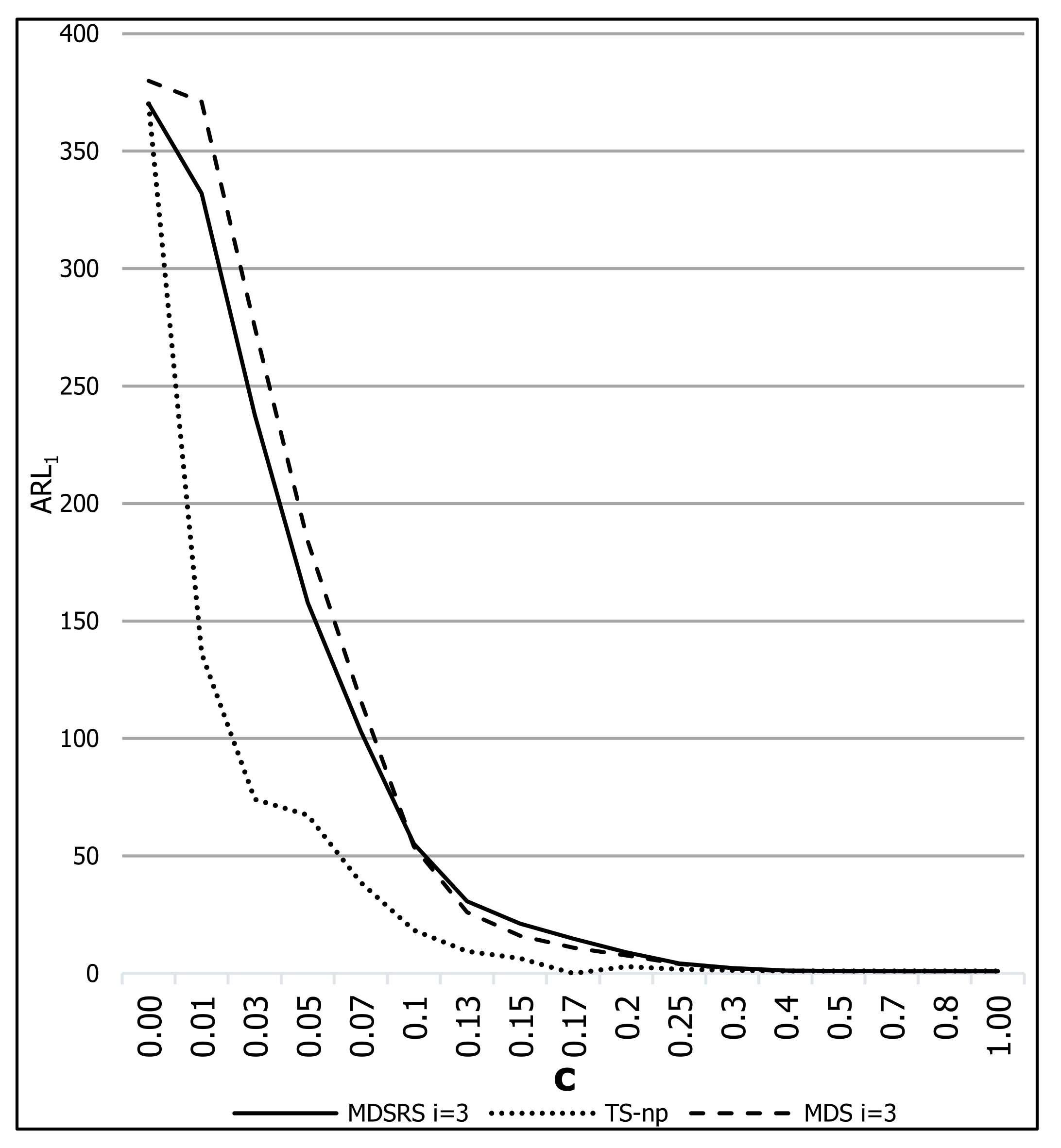


