Dominating Broadcasts in Fuzzy Graphs

Abstract

Broadcasting problems in graph theory play a significant role in solving many complicated physical problems. However, in real life there are many vague situations that sometimes cannot be modeled using usual graphs. Consequently, the concept of a fuzzy graph $G_F:(V,\sigma ,\mu )$ has been introduced to deal with such problems. In this study, we are interested in defining the notion of dominating broadcasts in fuzzy graphs. We also show that, in a connected fuzzy graph containing more than one element in ${\sigma }^{*}$, a dominating broadcast always exists, where ${\sigma }^{*}$ is $\{v\in V|\sigma \left(v\right)>0\}$. In addition, we investigate the relationship between broadcast domination numbers, radii, and domination numbers in a fuzzy graph as follows; ${\gamma }_b\left(G_F\right)\le min\{r\left(G_F\right),\gamma \left(G_F\right)\}$, where ${\gamma }_b\left(G_F\right)$ is the broadcast domination number, $r\left(G_F\right)$ is the radius, and $\gamma \left(G_F\right)$ is domination numbers in fuzzy graph $G_F$, with $|{\sigma }^{*}|>1$.

1. Introduction

In mathematics, a graph, G, is a mathematical structure consisting of a nonempty set, $V\left(G\right)$, of vertices and a set, $E\left(G\right)$, of edges. If there is an edge between two vertices, u and v, in $V\left(G\right)$, then we say that u and v are adjacent. Additionally, if u and v are distinct vertices in G, then a $u-v$ path of length n is a finite sequence of distinct vertices $u=u_0,u_1,u_2,\dots ,u_n=v$, such that vertices $u_{i-1}$ and $u_i$ are adjacent where $i\in \{1,2,3,\dots ,n\}$. A $u-v$ path with the minimum possible length is called the shortest path from u to v, and its length is denoted by $d(u,v)$. If there is no path from u to v, then $d(u,v)$ is ∞. In addition to this, $d(u,u)=0$ for all $u\in V\left(G\right)$. A graph, G, is said to be connected if there is a path between any two distinct vertices in G. Otherwise, G is said to be disconnected. In a connected graph G, the eccentricity of a vertex, $v\in V\left(G\right)$, is defined as $e\left(v\right)$ = $max\left\{d(u,v)|u\in V(G)\right\}$, and the diameter of G is defined as $diam\left(G\right)=max\left\{e\right(v\left)\right|v\in V\left(G\right)\}$. Moreover, a function $f:V\left(G\right)\to \{0,1,2,\dots ,diam(G\left)\right\}$ is called a broadcast if $f\left(v\right)\le e\left(v\right)$ for each vertex v in $V\left(G\right)$.

Graph theory was first developed by Euler [1] in 1736 who studied the Königsberg bridge problem. Since then, graph theory has become widely known. A graph can be applied to a model in communication, data network, and the science, such as biology, chemistry, and computer science [2,3]. Graph theory is considered to be a tool that can be used to solve optimization problems such as selecting routes which may be longer but less cost in a communication network. Broadcasts [4,5] in graphs have played an important role in solving these problems. For example, the least number of Wi-Fi routers must be set in a building, so that every room in the building can receive a Wi-Fi signal while minimizing expenses. This problem can be represented by a graph whose vertices represent the locations of the Wi-Fi routers in the building. If the distance between any two vertices does not exceed the limit of signal transportation, then there is an edge joining them. The suitable positions of Wi-Fi routers in this problem can be determined using broadcasts in graphs. However, broadcasts in usual graphs cannot solve certain real life problems, because, sometimes, there are some vague data that have to be considered in constructing a graph model for a problem. Uncertainty theories have been developed to find an answer to such problems. One concept developed in such theories that has been studied and applied to various physical problems is known as the “fuzzy set”.

Fuzzy sets were firstly introduced by Zadeh [6] in 1965. He noticed that the memberships of some classes of objects in the real world are not exactly imposed. For instance, dogs, cats, and birds obviously fall under the class of ’animals’, whereas starfish and bacteria cannot be characterized. Similarly, the class of ’beautiful women’ or the class of ’tall men’ cannot be identified as classes in mathematical terms. However, these characterizations can be completed by human thinking rules. Firstly, the notion of a fuzzy graph was introduced by Kauffman [7] in 1973, that study used the fuzzy relations, defined by Zadeh [8] in 1971, on classical sets. Later, in 1975, Rosenfeld [9] showed that fuzzy relations defined on fuzzy sets can have practical uses with graphs, and this led to generalizing the definition of fuzzy graphs. He combined his knowledge about fuzzy sets and graph theory to introduce the notion of a fuzzy graph. A fuzzy graph is a triple $(V,\sigma ,\mu )$, where V is a nonempty set, $\sigma :V\to [0,1]$ and $\mu :V\times V\to [0,1]$, such that for any $u,v\in V$, $\mu (u,v)\le min\left\{\sigma \right(u),\sigma (v\left)\right\}$. He also developed the theory of fuzzy graphs. After that, fuzzy graph theory became an important area of mathematical research, presenting networks with ambiguity. The benefits of fuzzy graphs are widely studied in various aspects and applied in various fields. In 2013, Dey and Pal [10] designed a traffic network using a fuzzy graph model. This traffic network helps to reduce the waiting time of conveyance on the road. In 2015, Lytvynenko et al. [11] used a fuzzy graph theory to find the traveling times over short distances of an army. They determined the values of the slope of the road and the obstacles to travel as a membership function and solved the problem of finding the optimal route using fuzzy graphs. In 2011, Gani [12] studied domination, independent domination, and irredundance using a fuzzy graph, $G_F$. In addition, she demonstrated the relationship between parameters $ir\left(G_F\right)$, $\gamma \left(G_F\right)$, and $i\left(G_F\right)$, where $ir\left(G_F\right)$ is the minimum cardinality taken over all maximal irredundant sets of $G_F$, $\gamma \left(G_F\right)$ is the minimum cardinality taken from all minimal dominating sets of $G_F$, and $i\left(G_F\right)$ is the minimum cardinality taken over all maximal independent dominating sets of $G_F$, respectively. Later, in 2014, Tom and Sunitha [13] proposed the notion of a fuzzy graph for measuring eccentricity, radius, diameter, and some of their properties. Afterward, in 2015, Manjusha and Sunitha [14] discovered the notion of strong domination using membership values of strong arcs in fuzzy graphs.

In this study, we are interested in defining the notion of dominating broadcasts in fuzzy graphs. We show that, in a connected fuzzy graph containing more than one element in ${\sigma }^{*}$, a dominating broadcast always exists. In addition, we investigate the relationship between ${\gamma }_b\left(G_F\right)$, $\gamma \left(G_F\right)$, and $r\left(G_F\right)$, where ${\gamma }_b\left(G_F\right)$, $\gamma \left(G_F\right)$, and $r\left(G_F\right)$ are defined as the broadcast domination number, domination number, and radius in $G_F$, respectively.

2. Preliminaries

In this section, we provide fundamental definitions used when discussing fuzzy graphs and their related essentials. Throughout this paper, let $G_F:(V,\sigma ,\mu )$ be a fuzzy graph, where V is a nonempty set, $\sigma :V\to [0,1]$ is a membership function of V, and $\mu :V\times V\to [0,1]$ is a fuzzy relation of V, such that $\mu (u,v)\le min\left\{\sigma \right(u),\sigma (v\left)\right\}$, for all $u,v\in V$. We assume that V is finite and nonempty and that $\mu$ is anti-reflexive and symmetric. An ordered pair, $(u,v)\in V\times V$, is called an arc. When the value of a membership function is zero, it shows nonexistence. So, the vertices v whose $\sigma \left(v\right)=0$ and the arc $(u,v)$ whose $\mu (u,v)=0$ will not be considered in a fuzzy graph, as discussed in [13]. 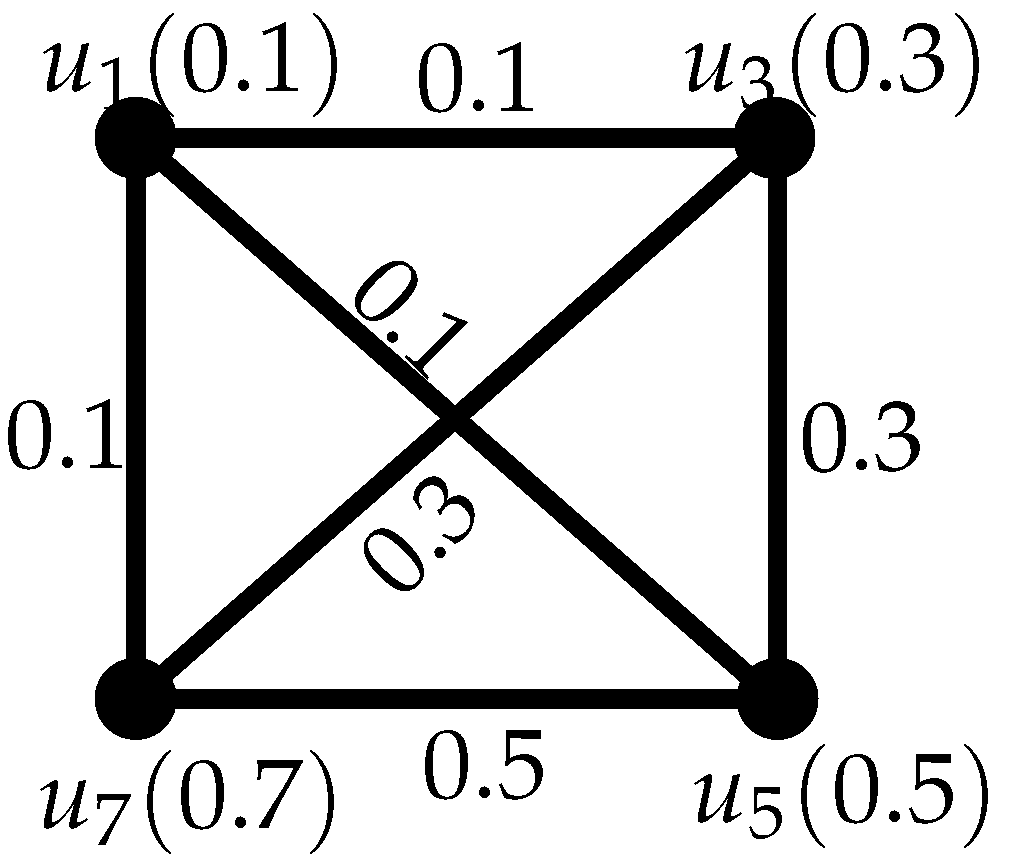For simplicity, a fuzzy graph, $G_F:(V,\sigma ,\mu )$, is written referred to as $G_F$ throughout this paper, unless explicitly stated otherwise. For example, let $V=\{u_1,u_2,\dots ,u_7\}$ and $\sigma :V\to [0,1]$ be defined by

$$\sigma \left(u_i\right)=\left\{\begin{array}{cc}\frac{i}{10}\hfill & \mathrm{if}i\mathrm{is}\mathrm{odd},\hfill \\ 0\hfill & \mathrm{otherwise},\hfill \end{array}\right.$$

for all $1\le i\le 7$. Let $\mu :V\times V\to [0,1]$ be defined by $\mu (u_i,u_j)=min\{\sigma \left(u_i\right),\sigma \left(u_j\right)\}$ for all $1\le i<j\le 7$. The picture of this fuzzy graph is shown in Figure 1. The underlying crisp graph of a fuzzy graph $G_F$ is denoted by $G_F^{*}:({\sigma }^{*},{\mu }^{*})$, where ${\sigma }^{*}=\{u\in V|\sigma \left(u\right)>0\}$ and ${\mu }^{*}=\{(u,v)\in V\times V|\mu (u,v)>0\}.$

A path of length n in a fuzzy graph $G_F:(V,\sigma ,\mu )$ is a sequence of distinct elements, $u_0,u_1,u_2,\dots ,u_n$ in V, such that $\mu (u_{i-1},u_i)>0$ for all $i\in \{1,2,3,\dots ,n\}$. The strength of a sequence of distinct elements $u_0,u_1,\dots ,u_n$ in V is $min\left\{\mu (u_{i-1},u_i)\right|i\in \{1,2,3,\dots ,n\}\}$.

The strength of connectedness between two vertices, u and v, in a fuzzy graph $G_F$, denoted by $CON{N}_{G_F}(u,v)$, is defined as the maximum of the strengths of all the sequences of distinct elements $u_0,u_1,u_2,\dots ,u_n$ in V, such that $u_0=u$ and $u_n=v$. For example, let $G_F$ be a fuzzy graph as shown in Figure 1. Then, $CON{N}_{G_F}(u_3,u_7)=0.3$. The fuzzy graph $G_F$ is said to be connected if $CON{N}_{G_F}(u,v)>0$ for all $u,v\in {\sigma }^{*}$. Otherwise, $G_F$ is said to be disconnected. Notice that the fuzzy graph in Figure 1 is connected.

In this study, we focus only on connected fuzzy graphs. So we assume throughout that $G_F$ is a connected fuzzy graph. The distance between two vertices u and v in $G_F$, denoted by $d_s(u,v)$, is defined by

$$d_s(u,v)=min\left\{\sum _{i=1}^n\mu (u_{i-1},u_i)|u=u_0,u_1,u_2,\dots ,u_n=v\mathrm{is}\mathrm{a}\mathrm{path}\mathrm{in}{G}_F\right\}.$$

In particular, $d_s(u,u)=0$ for all $u\in {\sigma }^{*}$. One can regard $d_s$ as a function from ${\sigma }^{*}\times {\sigma }^{*}$ to $[0,\infty )$. The eccentricity of a vertex $v\in {\sigma }^{*}$ is defined as $e_F\left(v\right)=max\left\{d_s(u,v)\right|u\in {\sigma }^{*}\}$. In other words, the eccentricity is the maximum distance from v to any vertex in ${\sigma }^{*}$. The radius and diameter of $G_F$ are defined as $r\left(G_F\right)=min\left\{e_F\left(v\right)\right|v\in {\sigma }^{*}\}$ and $dia{m}_F\left(G_F\right)=max\left\{e_F\left(v\right)\right|v\in {\sigma }^{*}\}$, respectively. One can see that the concepts of distance, eccentricity, radius, and diameter are similar to the usual ones defined in graph theory. As mentioned in the previous section, we are interested in studying the concepts of broadcasts and dominating broadcasts in fuzzy graphs. However, the definition of broadcasts in fuzzy graphs has not yet been defined. So, we will introduce the notion of broadcasts and study their properties in the next section.

3. Results

In this section, we introduce the definitions of broadcasts and dominating broadcasts of fuzzy graphs in Section 3.1. We show the relationship between $\gamma \left(G_F\right)$, ${\gamma }_b\left(G_F\right)$, and $r\left(G_F\right)$, where $\gamma \left(G_F\right)$ is the domination numbers, ${\gamma }_b\left(G_F\right)$ is the broadcast domination number, and $r\left(G_F\right)$ is the radius in $G_F$, in Section 3.2.

3.1. Broadcasts and Dominating Broadcasts in Fuzzy Graphs

Definition 1.

Let $G_F$ be a fuzzy graph containing more than one element in ${\sigma }^{*}$. For each $v\in {\sigma }^{*}$, define

$$ms\left(v\right)=min\left\{strengthofP\right|Pis\mathrm{a}pathfromvtoa\mathit{vertex}u\in {\sigma }^{*}-\left\{v\right\}\}.$$

Note that $min\left\{\mathit{strength}\mathit{of}P\right|P\mathit{is}a\mathit{path}\mathit{from}v\mathit{to}u\}\le d_s(v,u)$, and thus, $ms\left(v\right)\le d_s(v,u)$ for all $u\in {\sigma }^{*}-\left\{v\right\}$. Therefore, $ms\left(v\right)\le max\left\{d_s(v,u)\right|u\in {\sigma }^{*}-\left\{v\right\}\}=e_F\left(v\right)$.

Definition 2.

Let $G_F$ be a fuzzy graph. A function $f:{\sigma }^{*}\to [0,dia{m}_F\left(G_F\right)]$ is a broadcast in $G_F$ if either $f\left(v\right)=0$ or $ms\left(v\right)\le f\left(v\right)\le e_F\left(v\right)$ for all $v\in {\sigma }^{*}$.

According to the definition of broadcasts in fuzzy graphs proposed in this work, we need any broadcast, f, mapping each vertex, v, to equal 0, which means this vertex cannot send a signal to other vertices in the graph or that $ms\left(v\right)\le f\left(v\right)$ can ensure that at least one vertex in the graph can receive a signal from v through a connecting path.

Definition 3.

The cost of a broadcast f in a fuzzy graph $G_F$ is defined as $\sum \left(f\right)={\sum }_{v\in {\sigma }^{*}}f\left(v\right)$.

One can see that there can be more than one broadcast in a fuzzy graph. Let $G_F:(V,\sigma ,\mu )$ be a fuzzy graph containing more than one element in ${\sigma }^{*}$. Let $v\in {\sigma }^{*}$ be given. One can define $f\left(v\right)=e_F\left(v\right)$ and $f\left(u\right)=0$ for all $u\in {\sigma }^{*}-\left\{v\right\}$. Then, f is a broadcast. If $x\in {\sigma }^{*}-\left\{v\right\}$, then we can define another broadcast, $g:{\sigma }^{*}\to [0,dia{m}_F\left(G_F\right)]$, by $g\left(x\right)=e_F\left(x\right)$ and $g\left(u\right)=0$ for all $u\in {\sigma }^{*}-\left\{x\right\}$. As a result, there are at least two broadcasts in $G_F$.

Definition 4.

Let f be a broadcast in a fuzzy graph $G_F$. A vertex v in ${\sigma }^{*}$ is called a broadcast vertex if $f\left(v\right)>0$. The set of all broadcast vertices of $G_F$ is denoted by ${\sigma }_{f^{+}}^{*}$.

Definition 5.

A broadcast f in a fuzzy graph $G_F$ is called a  dominating broadcast if for each vertex, u, in ${\sigma }^{*}$, there exists a vertex, $v\in {\sigma }_{f^{+}}^{*}$, such that $d_s(u,v)\le f\left(v\right)$.

For each $v\in {\sigma }^{*}$, define $f:{\sigma }^{*}\to [0,dia{m}_F\left(G_F\right)]$ by $f\left(v\right)=e_F\left(v\right)$ and $f\left(u\right)=0$, for all $u\in {\sigma }^{*}-\left\{v\right\}$. Then, f is a broadcast in $G_F$, such that ${\sigma }_{f^{+}}^{*}=\left\{v\right\}$. Moreover, $d_s(u,v)\le e_F\left(v\right)=f\left(v\right)$ for all $u\in {\sigma }^{*}$. Therefore, f dominates. As a result, there exists a dominating broadcast in a connected fuzzy graph containing more than one vertex in ${\sigma }^{*}$.

If $G_F$ is a fuzzy graph with only one vertex in ${\sigma }^{*}$, then $dia{m}_F\left(G_F\right)=0$. This implies that there is only one broadcast on $G_F$ in which $f\left({\sigma }^{*}\right)=\left\{0\right\}$. However, this broadcast is not a dominating broadcast, because ${\sigma }_{f^{+}}^{*}=\varnothing$.

3.2. The Relationship between Domination Numbers and Radius in Fuzzy Graphs

In this section, we demonstrate the relationship between domination numbers and radius in fuzzy graphs.

Definition 6

([13]). An arc of a fuzzy graph is called strong if its membership function value is at least as great as the strength of the connectedness between its endpoints when it is deleted.

Definition 7

([12]). Let $G_F$ be a fuzzy graph. A subset D of ${\sigma }^{*}$ is said to be a fuzzy dominating set of $G_F$ if, for every $v\in {\sigma }^{*}-D$, there exists $u\in D$, such that $(u,v)$ is a strong arc.

Definition 8

([12]). A fuzzy dominating set, D, of a fuzzy graph, $G_F$, is called a minimal dominating set of $G_F$, if, for every vertex $v\in D,$ the set $D-\left\{v\right\}$ is not a dominating set.

Theorem 1.

Let $G_F$ be a connected fuzzy graph containing more than one vertex in ${\sigma }^{*}$. Then, for each $v\in {\sigma }^{*}$, the set ${\sigma }^{*}-\left\{v\right\}$ is a fuzzy dominating set of $G_F$.

Proof. 

Let $v\in {\sigma }^{*}$. As $|{\sigma }^{*}|>1$, we have ${\sigma }^{*}-\left\{v\right\}\ne \varnothing$. Moreover, $\{u\in {\sigma }^{*}|\mu (u,v)>0\}\ne \varnothing$ because $G_F$ is connected. Let $u\in {\sigma }^{*}-\left\{v\right\}$ be such that $\mu (u,v)=max\left\{\mu (a,v)\right|a\in {\sigma }^{*}\}$. Then, $CON{N}_G(v,u)\le \mu (v,u)$. Therefore, $(u,v)$ is strong and, thus, ${\sigma }^{*}-\left\{v\right\}$ is a fuzzy dominating set. □

Let $G_F$ be a connected fuzzy graph containing more than one vertex in ${\sigma }^{*}$. As a result of Theorem 1, there always exists a minimal dominating set which is not ${\sigma }^{*}$.

Definition 9

([12]). The domination number$\gamma \left(G_F\right)$ is the minimum number of cardinalities taken over all minimal dominating sets of $G_F$.

Definition 10.

The broadcast domination number of $G_F$, denoted by ${\gamma }_b\left(G_F\right)$, is $inf\{\sum (f)$|f, which is a dominating broadcast of $G_F\}$.

Proposition 1.

Let $G_F$ be a connected fuzzy graph containing more than one vertex in ${\sigma }^{*}$. Then,

$${\gamma }_b\left(G_F\right)\le r\left(G_F\right).$$

Proof. 

Let $v\in {\sigma }^{*}$ be such that $e_F\left(v\right)=r\left(G_F\right)$. We define $f:{\sigma }^{*}\to [0,dia{m}_F\left(G_F\right)]$ by:

$$f\left(x\right)=\left\{\begin{array}{ccc}r\left(G_F\right)\hfill & \mathrm{if}& x=v,\hfill \\ 0\hfill & \mathrm{if}& x\ne v,\hfill \end{array}\right.$$

for all $x\in {\sigma }^{*}$. From this, $0\le r\left(G_F\right)\le dia{m}_F\left(G_F\right)$. For each $x\in {\sigma }^{*}$, if $x=v$, then $f\left(x\right)=r\left(G_F\right)=e_F\left(v\right)\ge ms\left(v\right)$ and, if $x\ne v$, then $f\left(x\right)=0$. Therefore, f is a broadcast. For each $x\in {\sigma }^{*}$, we have $d_s(x,v)\le e_F\left(v\right)=r\left(G_F\right)=f\left(v\right)$. Then, $d_s(x,v)\le f\left(v\right)$ for all $x\in {\sigma }^{*}$. Therefore, f is a dominating broadcast. Since $\sum \left(f\right)={\sum }_{v\in {\sigma }_{f^{+}}^{*}}f\left(v\right)=r\left(G_F\right)$, we have ${\gamma }_b\left(G_F\right)\le \sum \left(f\right)=r\left(G_F\right)$. Therefore, ${\gamma }_b\left(G_F\right)\le r\left(G_F\right)$. □

Proposition 2.

Let $G_F$ be a connected fuzzy graph containing more than one vertex in ${\sigma }^{*}$. Then:

$${\gamma }_b\left(G_F\right)\le \gamma \left(G_F\right).$$

Proof. 

First, from Definition 9, we can choose a fuzzy dominating set, S, of $G_F$, such that $\left|S\right|=\gamma \left(G_F\right)$. It follows from Theorem 1 that $S\ne {\sigma }^{*}$. Then, we define $f:{\sigma }^{*}\to [0,dia{m}_F\left(G_F\right)]$ by

$$f\left(v\right)=\left\{\begin{array}{cc}0\hfill & \mathrm{if}v\notin S,\hfill \\ min\{1,e_F\left(v\right)\}\hfill & \mathrm{if}v\in S,\hfill \end{array}\right.$$

for all $v\in {\sigma }^{*}$. Let $a\in {\sigma }^{*}$. If $a\in S$, we know that $f\left(a\right)=min\{1,e_F\left(a\right)\}\le e_F\left(a\right)\le dia{m}_F\left(G_F\right)$. If $a\notin S$, then $f\left(a\right)=0\le dia{m}_F\left(G_F\right)$. Hence, f is well defined. Notice that $ms\left(v\right)\le 1$ and $ms\left(v\right)\le e_F\left(v\right)$ for all $v\in {\sigma }^{*}$. It follows that, for each $v\in {\sigma }^{*}$, if $f\left(v\right)\ne 0$, then $ms\left(v\right)\le f\left(v\right)\le e_F\left(v\right)$. Therefore, f is a broadcast. We know that ${\sigma }_{f^{+}}^{*}=S$, since $G_F$ is connected. Next, we show that f is a dominating broadcast. Let $a\in {\sigma }^{*}$. If $a\in S$, then $a\in {\sigma }_{f^{+}}^{*}$, and $d_s(a,a)=0\le f\left(a\right)$. On the other hand, if $a\notin S$, then there is an element $b\in S$, such that $(a,b)$ is a strong arc. It follows that $b\in {\sigma }_{f^{+}}^{*}$, $d_s(a,b)\le \mu (a,b)\le 1$, and $d_s(a,b)\le e_F\left(b\right)$. This implies that $d_s(a,b)\le min\{1,e_F\left(b\right)\}=f\left(b\right)$. Therefore, f is a dominating broadcast. Note that ${\gamma }_b\left(G_F\right)\le {\sum }_{a\in {\sigma }_{f^{+}}^{*}}f\left(a\right)={\sum }_{a\in S}f\left(a\right)$. Moreover, for each $a\in S$, we know that $f\left(a\right)=min\{1,e_F\left(a\right)\}\le 1$. Thus, we obtain that ${\sum }_{a\in S}f\left(a\right)\le \left|S\right|$. It follows from Definition 10 that ${\gamma }_b\left(G_F\right)\le \left|S\right|$. Since $\left|S\right|=\gamma \left(G_F\right)$, we can conclude that ${\gamma }_b\left(G_F\right)\le \gamma \left(G_F\right)$. □

As a consequence of Propositions 1 and 2, we obtain the following result.

Theorem 2.

Let $G_F$ be a connected fuzzy graph containing more than one vertex in ${\sigma }^{*}$. Then, ${\gamma }_b\left(G_F\right)\le min\{r\left(G_F\right),\gamma \left(G_F\right)\}$.

3.3. An Application of Broadcasts in Fuzzy Graphs

In this section, we provide an example of applications of broadcasts in fuzzy graphs. The example refers to a problem concerning the suitability of the locations chosen to build the distribution centers (warehouses) of a manufacturer.

One of the concerns is reducing the transportation cost from the product manufacturer to the retail stores. The product manufacturer will only distribute the products to distribution centers. Then, each distribution center will deliver these products to retail stores [15]. There are five main factors to take into account when considering the suitability of the locations of warehouses. These factors consist of adequate spaces, customer services, favorable traffic, connections with suppliers and the retail stores, easy freeway accesses, and a qualified workforce [16]. The suitability degree measurement assists in designing the locations of the warehouses. On the other hand, if the unsuitability of any location is in the lowest degree, then these locations are qualified choices.

We assume that the manufacturer would like to distribute their products to seven cities, A, B, C, D, E, F, and G. An expert investigates all five factors of suitability and turns them into scores between 1 and 5 as follows:

An average score between 1.00–1.49 indicates the lowest suitability level.

An average score between 1.50–2.49 indicates a low suitability level.

An average score between 2.50–3.49 indicates a moderate suitability level.

An average score between 3.50–4.49 indicates a high suitability level.

An average score between 4.50–5.00 indicates the highest suitability level.

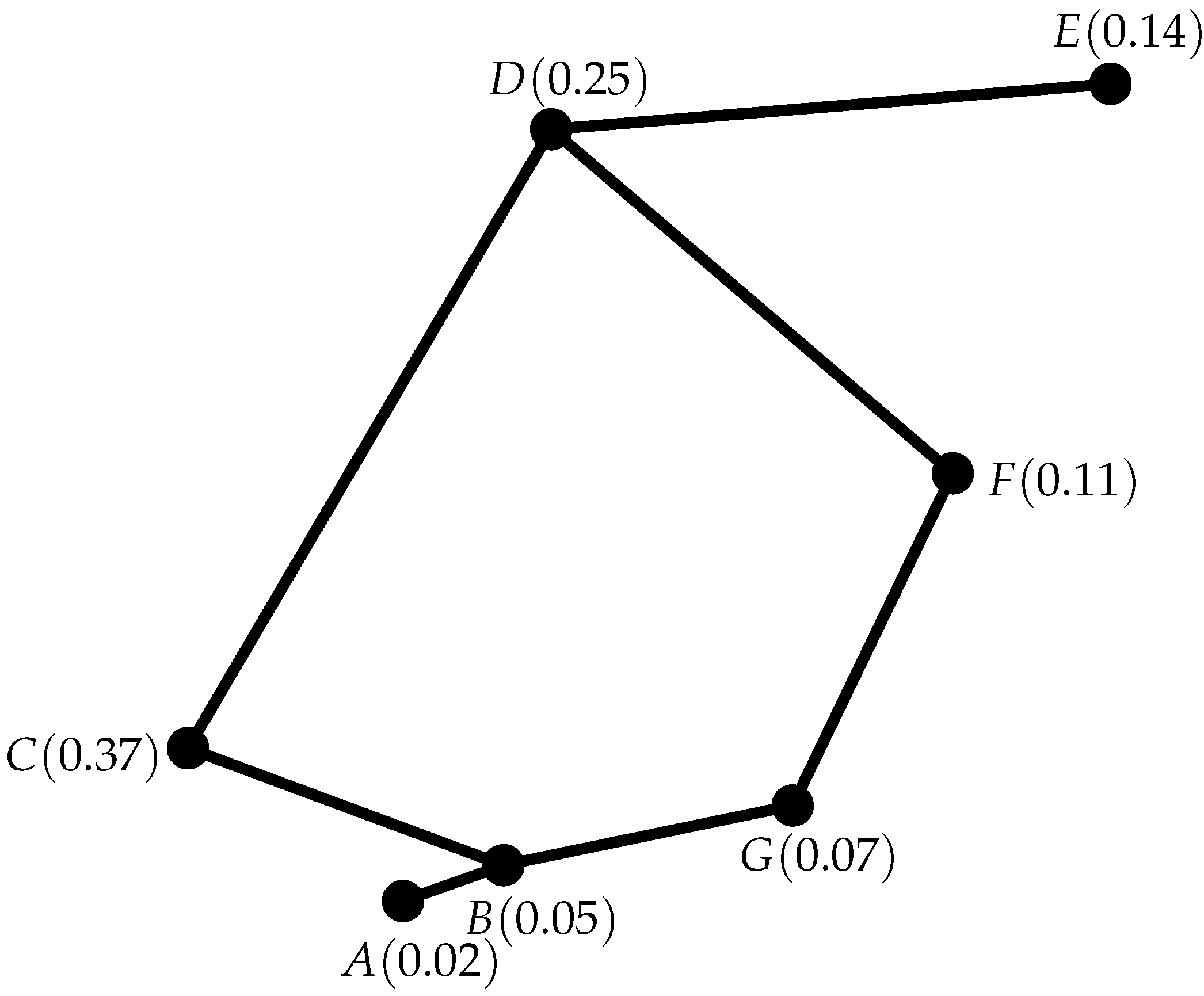
In order to apply the idea of broadcasts in fuzzy graphs to this situation, we let $V=\{A,B,C,D,E,F,G\}$. Then, we turn these scores into normalized average score between 0 to 1 of the unsuitability of the warehouse locations shown in Figure 2, using the function $\sigma :V\to [0,1]$ defined by

$$\sigma \left(x\right)=\left\{\begin{array}{cc}{e}^{1-s\left(x\right)}\hfill & \mathrm{if}s\left(x\right)\ge 1,\hfill \\ 1\hfill & \mathrm{otherwise},\hfill \end{array}\right.$$

for all $x\in V$, where $s\left(x\right)$ is the average score of suitability as shown in

Table 1. The average suitability and unsuitability scores of the warehouse locations.

Cities	Average Score of Suitability	Score of Unsuitability
A	4.9	0.02
B	4	0.05
C	2	0.37
D	2.4	0.25
E	3	0.14
F	3.2	0.11
G	3.6	0.07

. Next, we let $\mu$ be the degree of measurement of the available traveling path between any two considered cities. That is, $\mu :V\times V\to [0,1]$ is a function defined by:

$$\mu (a,b)=min\left\{\sigma \right(a),\sigma (b\left)\right\},$$

for all $a,b\in V$. Then, such defined functions and the set V make the triple $(V,\sigma ,\mu )$ be a fuzzy graph $G_F$. In order to find the most suitable warehouse location for this problem, we apply broadcasts in fuzzy graphs to this situation.

We consider the domination number of $G_F$. Notice that the minimum cardinalities taken over all minimal dominating sets of this fuzzy graph is 1. Moreover, from

Table 2. Present distance between two cities and eccentricity of each city.

Distance between Two Cities	A	B	C	D	E	F	G	Eccentricity of Each City
A	0	0.02	0.07	0.25	0.39	0.14	0.07	0.39
B	0.02	0	0.05	0.23	0.37	0.12	0.05	0.37
C	0.07	0.05	0	0.25	0.39	0.17	0.1	0.39
D	0.25	0.23	0.25	0	0.14	0.11	0.18	0.25
E	0.39	0.39	0.39	0.14	0	0.25	0.32	0.39
F	0.14	0.12	0.17	0.11	0.25	0	0.07	0.25
G	0.02	0.05	0.1	0.18	0.32	0.7	0	0.32

, we see that $r\left(G_F\right)=e_F\left(F\right)=0.25$. Moreover, $\left\{F\right\}$ is a minimal dominating set. It follows from Theorem 2 that ${\gamma }_b\left(G_F\right)\le min\{0.25,1\}$. Therefore, we obtain that ${\gamma }_b\left(G_F\right)\le 0.25$. The diameter of this fuzzy graph is 0.39. We can consider the cost of a fuzzy broadcast to be the damage of operating the warehouses at the vertices (i.e., cities) according to the broadcast. The damage can be considered to be the increased financial cost that the owner has to pay, the increased time-wasting in logistics, or the increase of environmental pollution caused by operating the warehouses at the selected places. If we define $f_1:V\to [0,0.39]$ by $f_1\left(F\right)=0.25,f_1\left(A\right)=0,f_1\left(B\right)=0,f_1\left(C\right)=0,f_1\left(D\right)=0,f_1\left(E\right)=0$, and $f_1\left(G\right)=0$, then $f_1$ is a broadcast in $G_F$ and ${\sigma }_{f_1^{+}}^{*}=\left\{F\right\}$. We know $d_s(a,F)\le e_F\left(F\right)$ for all $a\in V$. Hence, $f_1$ is a dominating broadcast. The cost of the broadcast $f_1$ is 0.25, which is a score of unsuitability. Note that the city whose value is $f_1$, attains a score of 0 in terms of suitability and will not be chosen as a warehouse. This means that, according to the values of $f_1$, we will choose the city F as a warehouse.

On the other hand, if we let $f_2$ be defined by $f_2\left(B\right)=0.05,f_2\left(D\right)=0.14,f_2\left(A\right)=0,f_2\left(C\right)=0,f_2\left(E\right)=0$, and $f_2\left(F\right)=0$, then $f_2$ is a broadcast in $G_F$, as shown in Figure 2. Moreover, $d_s(E,D)\le f_2\left(D\right),d_s(F,D)\le f_2\left(D\right),d_s(A,B)\le f_2\left(B\right),d_s(G,B)\le f_2\left(B\right)$, and $d_s(C,B)\le f_2\left(B\right)$, Therefore, $f_2$ is a dominating broadcast. The cost of the broadcast $f_2$ is 0.19, which is less than that of $f_1$. This implies that constructing warehouses in cities D and B will be more suitable than constructing a warehouse only in city F.

However, constructing two warehouse uses more money than constructing only one warehouse. Thus, the manufacturer needs to compare the benefits that they will receive in the long run.

4. Conclusions

In this work, we were interested in defining the concepts of broadcasts and dominating broadcasts in fuzzy graphs. In usual graph theory, these two concepts can be applied to minimize transportation problems and costs in communication networks. However, broadcasts in graphs cannot solve some real life problems because sometimes there are a few data that must be considered when constructing a graph model for a problem. As a consequence, we need the idea of fuzzy theory to deal with such complications in graph models. In Section 3, we proposed a definition of a broadcast in connected fuzzy graphs in Definition 2. We showed that there can be more than one broadcast in a connected fuzzy graph containing more than one vertex in ${\sigma }^{*}$. We also introduced the definition of dominating broadcasts in connected fuzzy graphs. We have proven that a dominating broadcast in a connected fuzzy graph containing more than one vertex in ${\sigma }^{*}$ exists. Moreover, it has been shown that there can be more than one dominating broadcast in a connected fuzzy graph. Afterward, we calculated the relationship between ${\gamma }_b\left(G_F\right),r\left(G_F\right)$, and $\gamma \left(G_F\right)$, where ${\gamma }_b\left(G_F\right)$ is the broadcast domination number, $r\left(G_F\right)$ is the radius, and $\gamma \left(G_F\right)$ is the broadcast domination number of a connected fuzzy graph $G_F$. The study shows the following inequality:

$${\gamma }_b\left(G_F\right)\le min\{r\left(G_F\right),\gamma \left(G_F\right)\}，$$

which is comparable to the one outlined in Erwin’s work [5].