
Recursive Identification for MIMO Fractional-Order Hammerstein Model Based on AIAGS

Abstract
:1. Introduction
2. Adaptive Immune Algorithm Based on Global Search Strategy
2.1. Review of Immune Algorithms
2.2. AIAGS
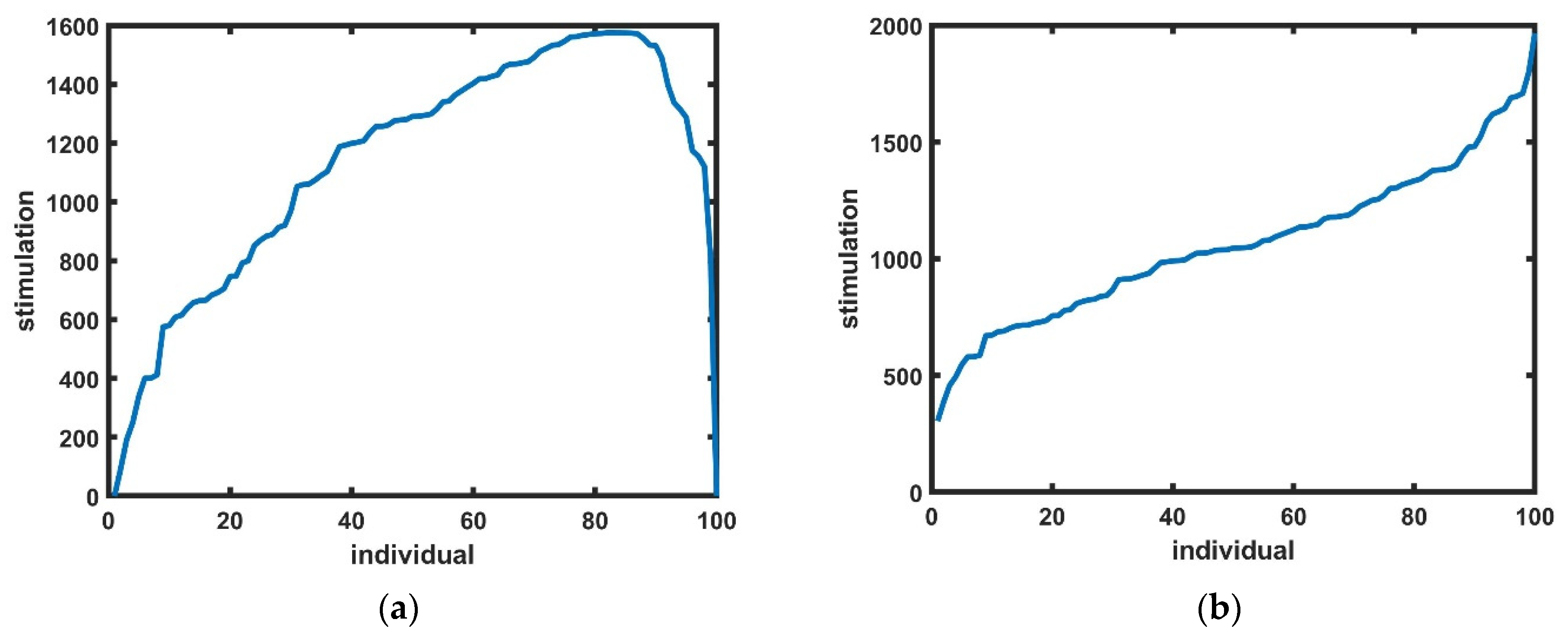
2.2.1. Stimulation Improvement
2.2.2. Mutation Strategy Improvement
2.2.3. Simulated Annealing Strategy
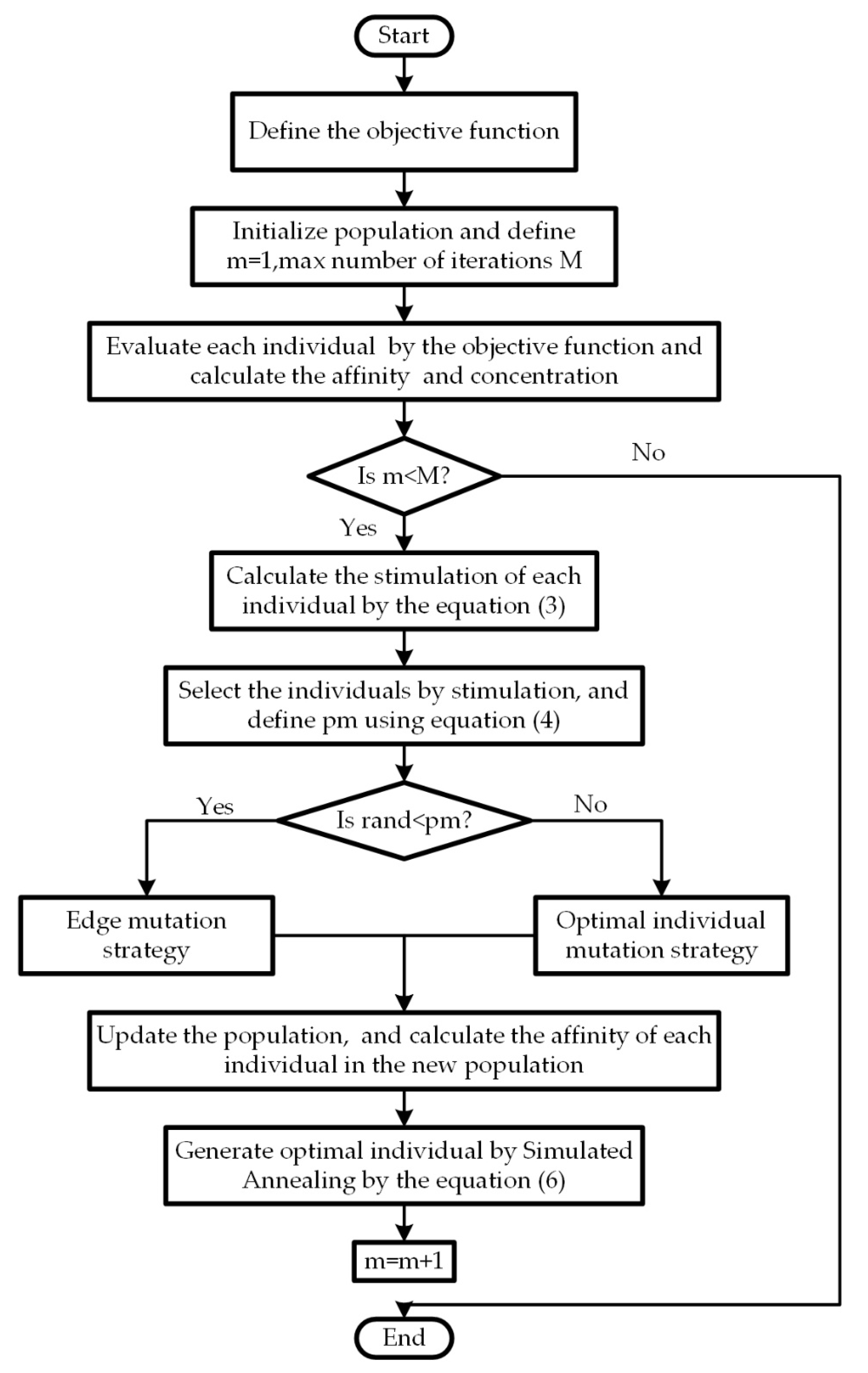
2.2.4. Pseudo Code of AIAGS
| Algorithm 1: AIAGS | |
| Step.1 | Define the objective function F; |
| Step.2 | Initialize population ; |
| Step.3 | Evaluate all the individuals by the objective function F; |
| Step.4 | Calculate the affinity and concentration of each individual; |
| Step.5 | Initialize the number of iteration ; |
| Step.6 | While < max number of iterations M; |
| Step.7 | Calculate the stimulation of each individual by the Equation (3); |
| Step.8 | Select the individuals in the population by stimulation and clone the individuals; |
| Step.9 | Mutate the cloned individuals by the Equation (5); |
| Step.10 | If the generated mutation vector exceeds the boundary, a new mutation vector is generated randomly until it is within the boundary; |
| Step.11 | Inhibit cloning and calculate the affinity of each new individual; |
| Step.12 | Generate optimal individual by Simulated Annealing by the Equation (6); |
| Step.13 | End; |
| Step.14 | ; |
| Step.15 | End while; |
| Step.16 | Return the best solution. |
2.3. Benchmark Function
2.3.1. Comparison of AIAGS with Other Algorithms
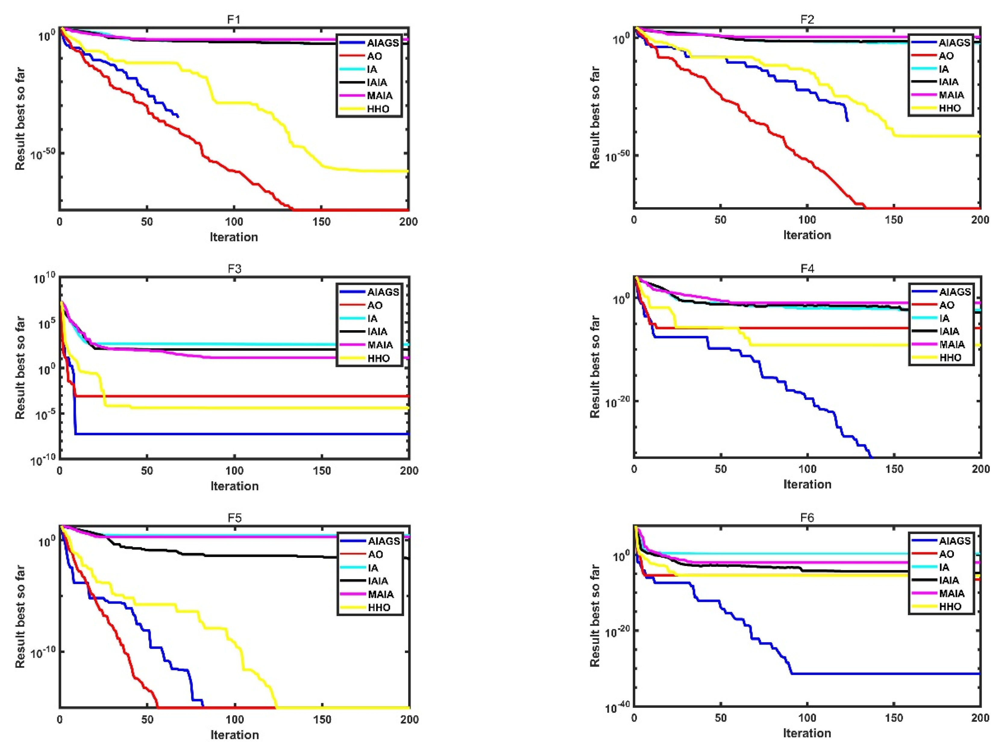
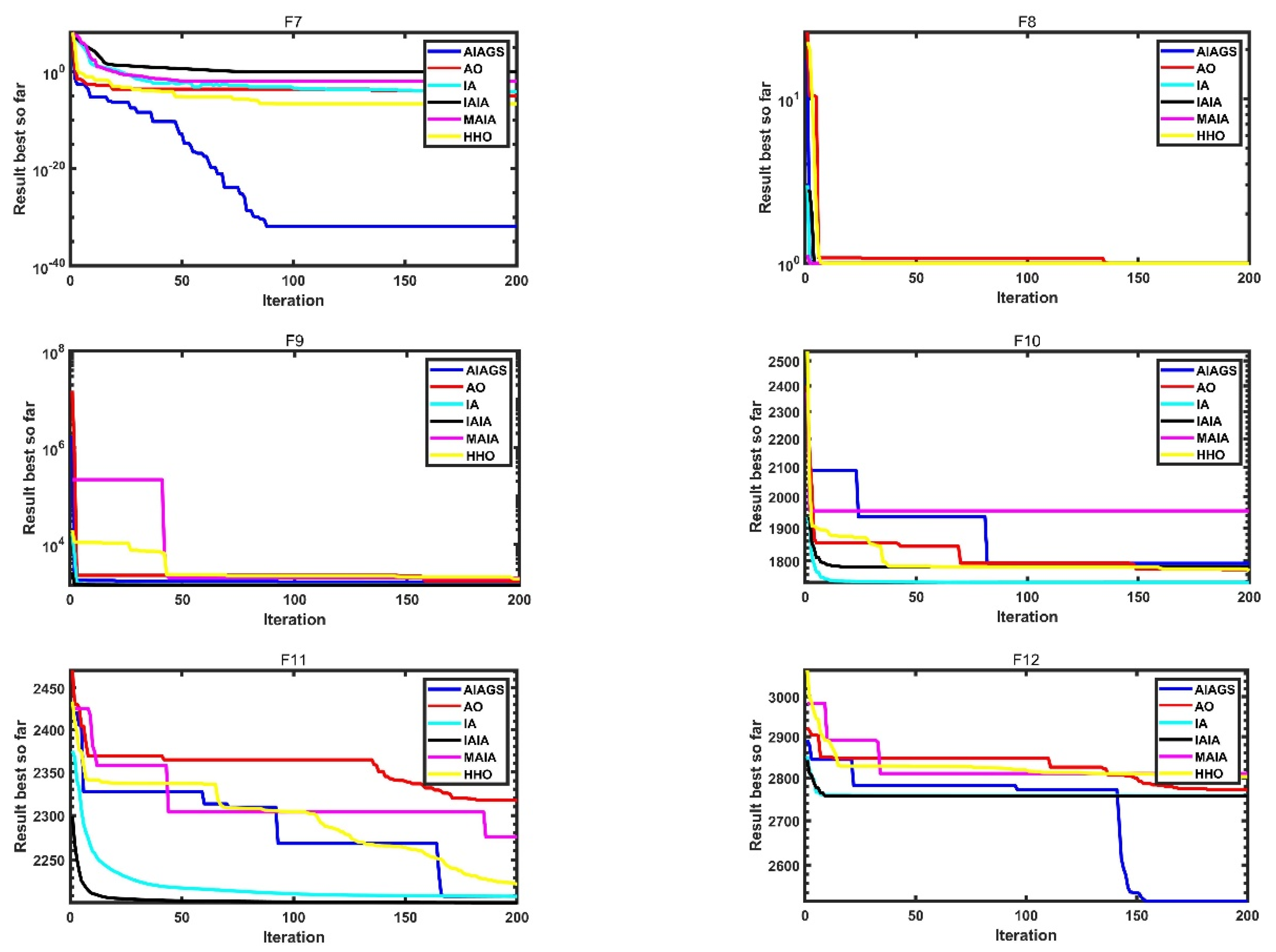
2.3.2. Convergence
2.4. Summary
3. Identification Method of MIMO Fractional Order Hammerstein Model
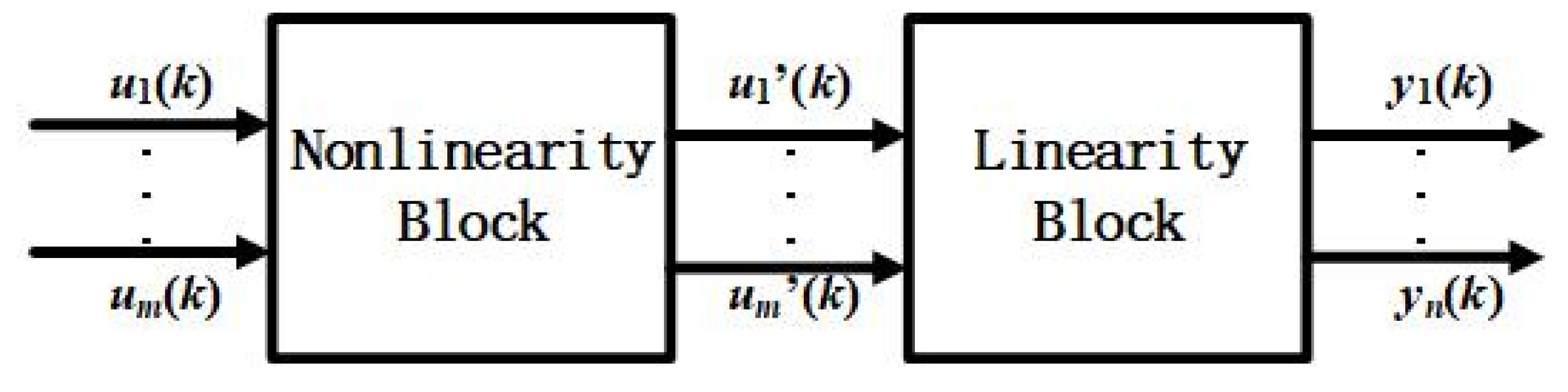
3.1. MIMO Fractional Order Hammerstein Model
3.1.1. Fractional Order Differentiation
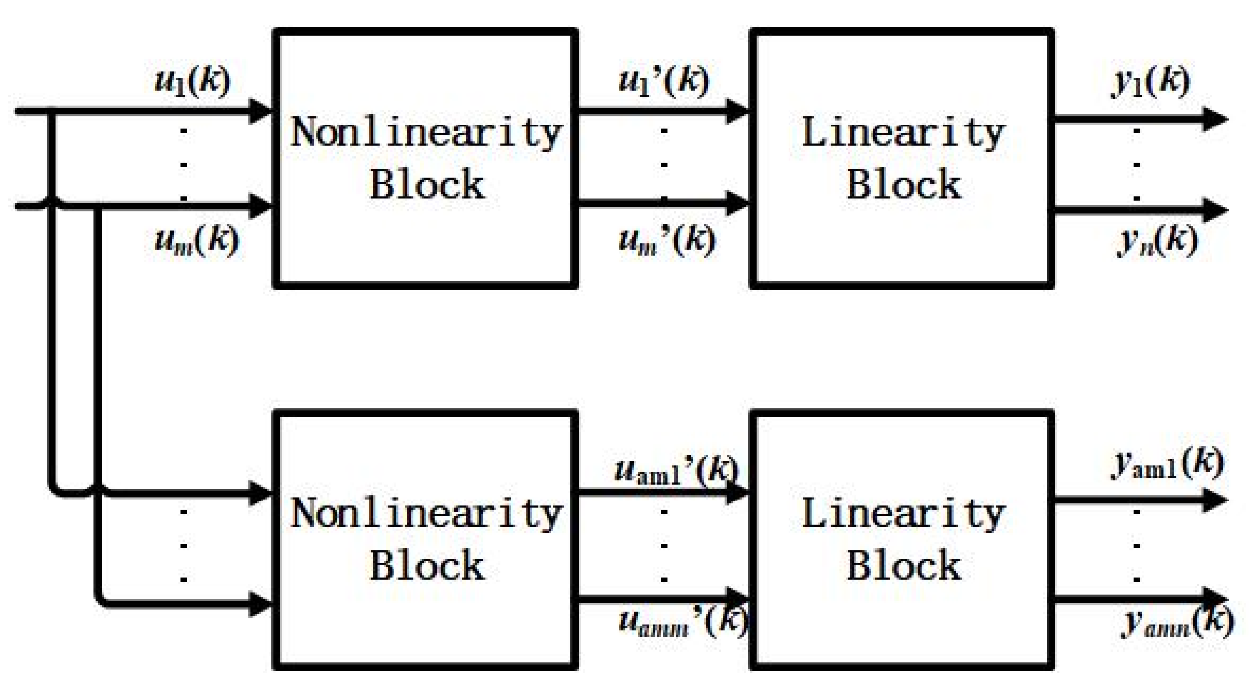
3.1.2. MIMO Fractional-Order Hammerstein System
3.2. Parameter Identification Based on Auxiliary Model Recursive Least Square Method
3.2.1. Coefficient Identification
3.2.2. Order Identification
3.3. Summary
4. Experimental Results
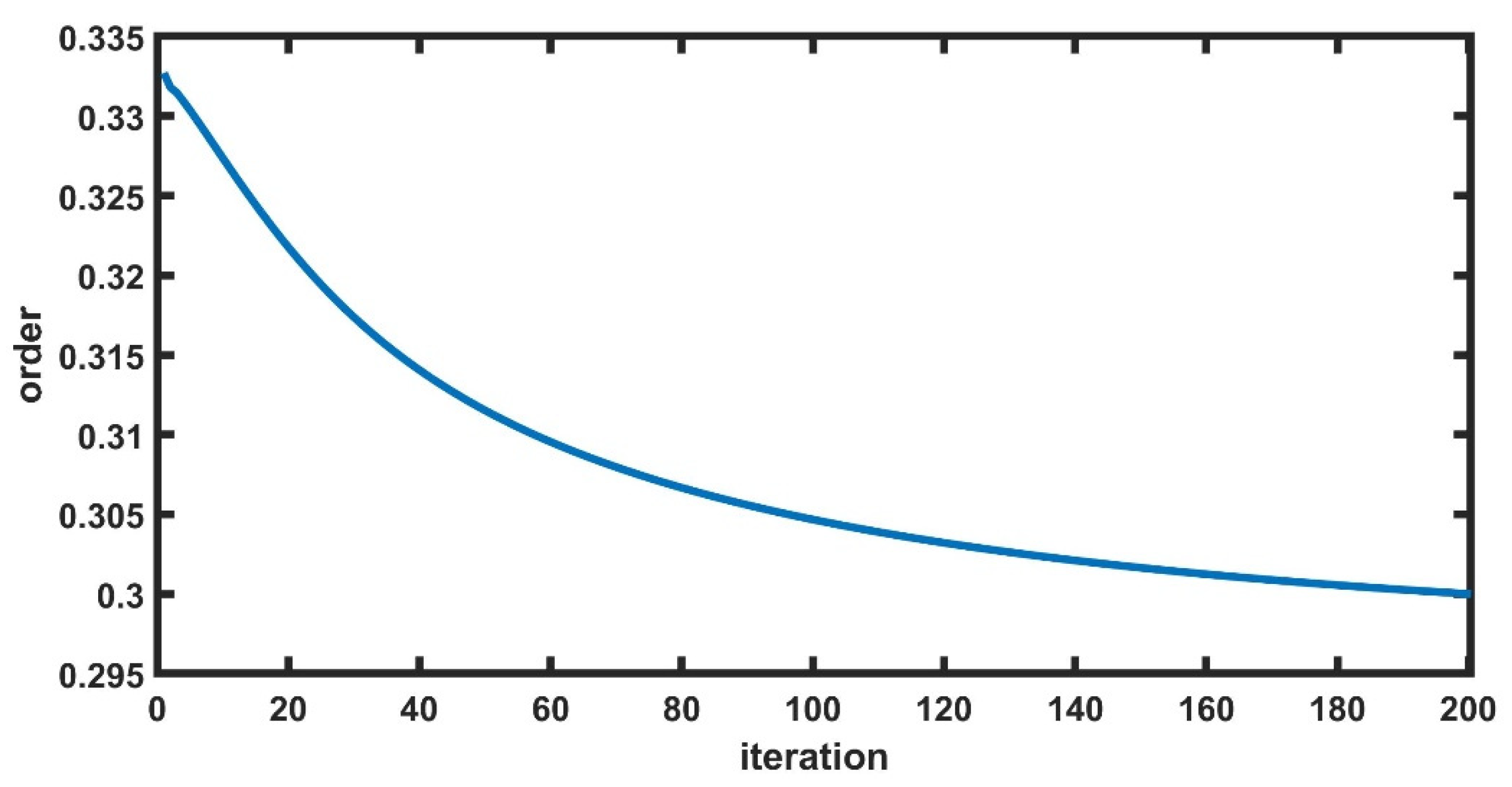
4.1. Example 1
| Algorithm 2: Identification process | |
| Step.1 | Collect the dates of all inputs, outputs; |
| Step.2 | Obtain the initial of unknown parameters by using intelligent optimization algorithm; |
| Step.3 | While < max number of iterations M; |
| Step.4 | Estimate the value of model coefficients according to Equation (25); |
| Step.5 | Estimate the value of fractional order according to Equation (29); |
| Step.6 | If the two criterion function values J within the actual accuracy requirements; |
| Step.7 | Break; |
| Step.8 | End; |
| Step.9 | ; |
| Step.10 | End while; |
| Step.11 | Return the best solution. |
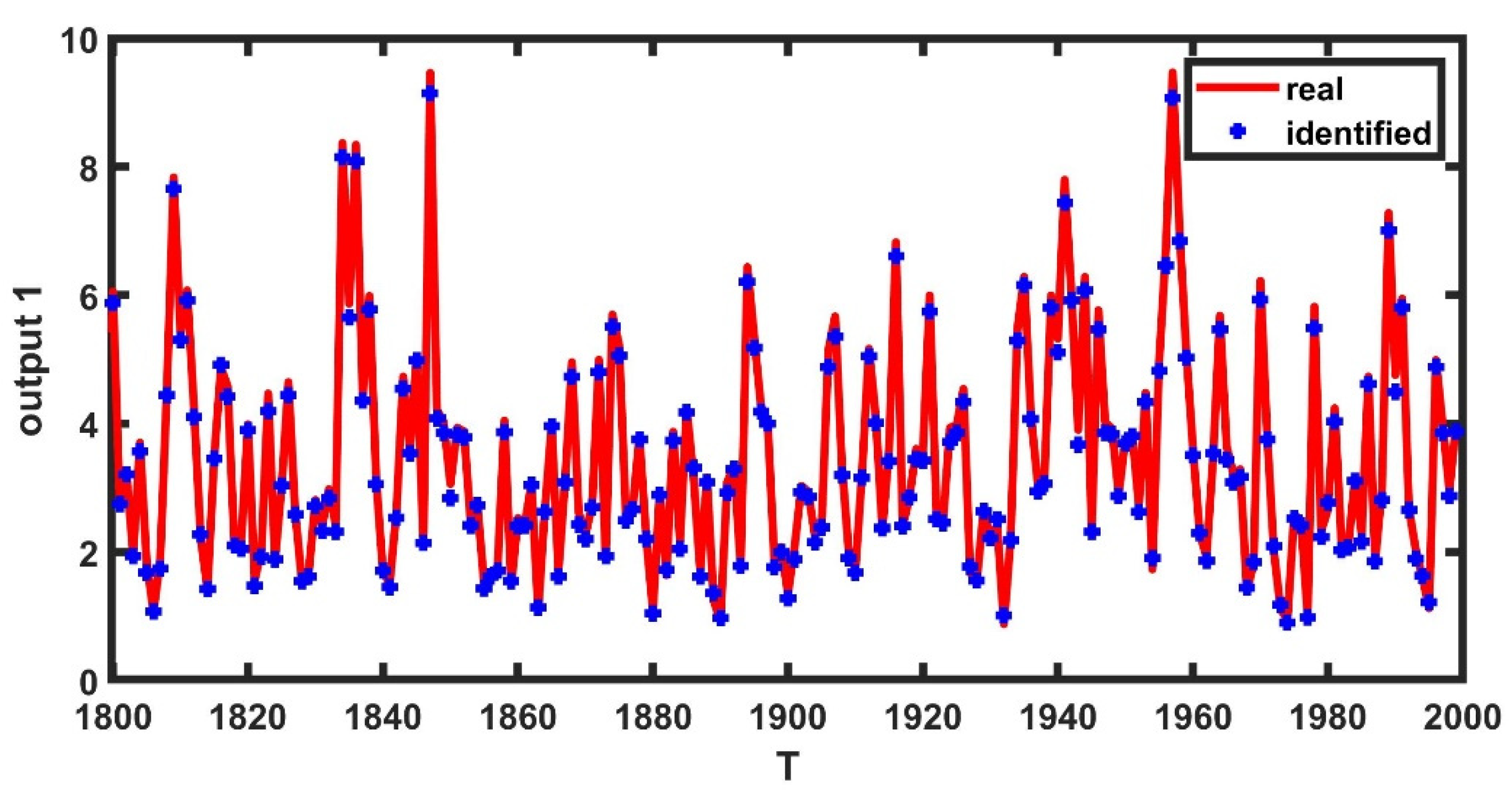
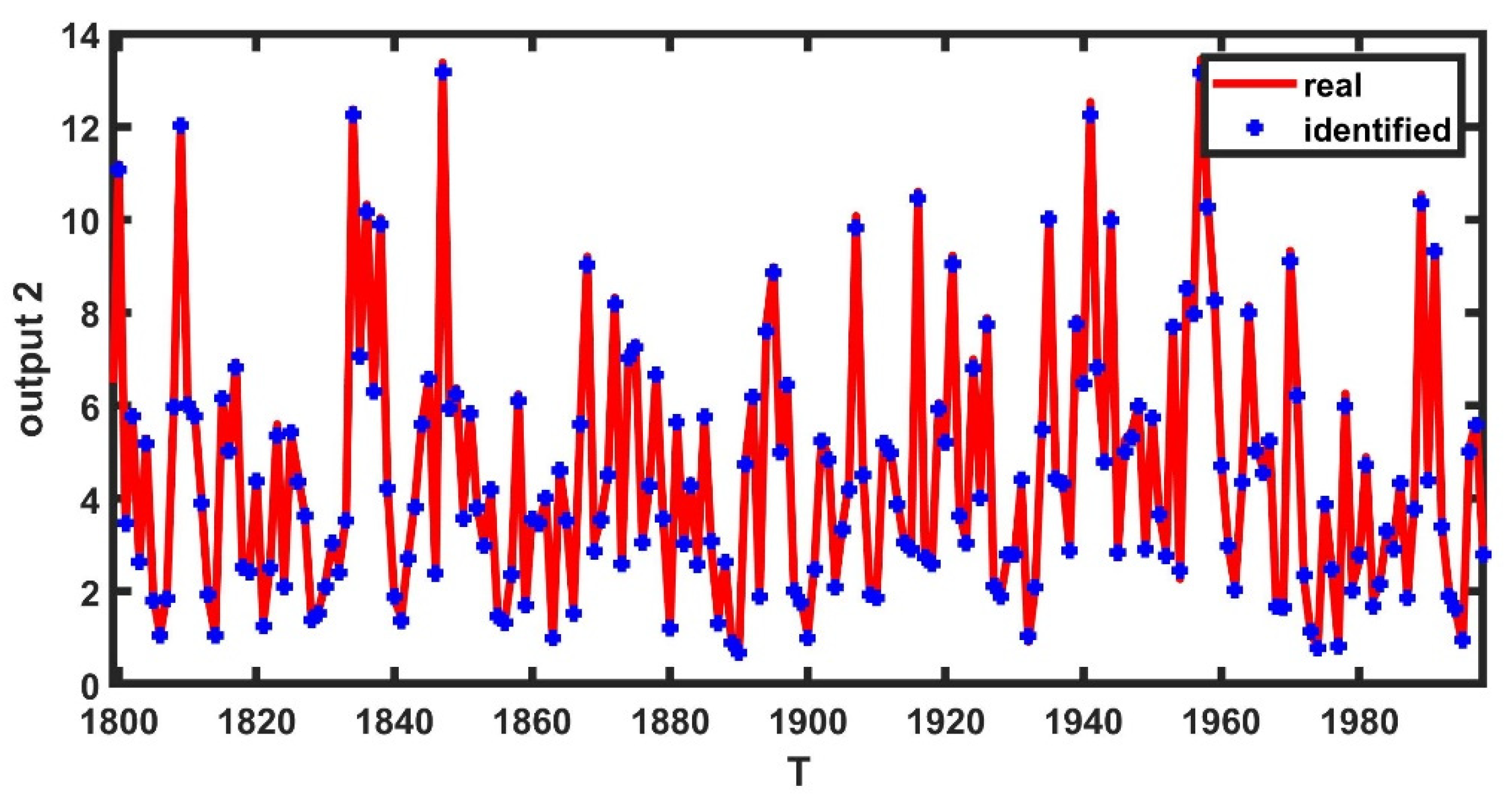
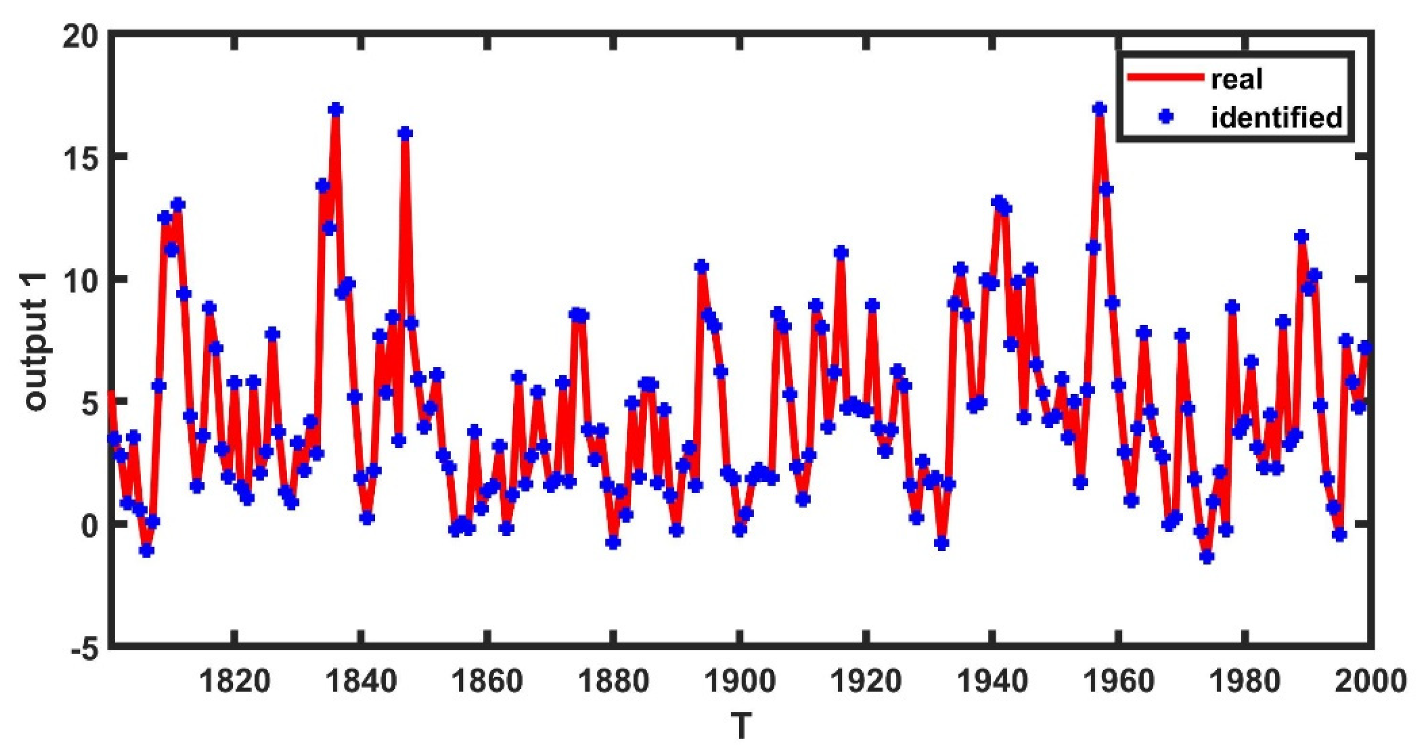
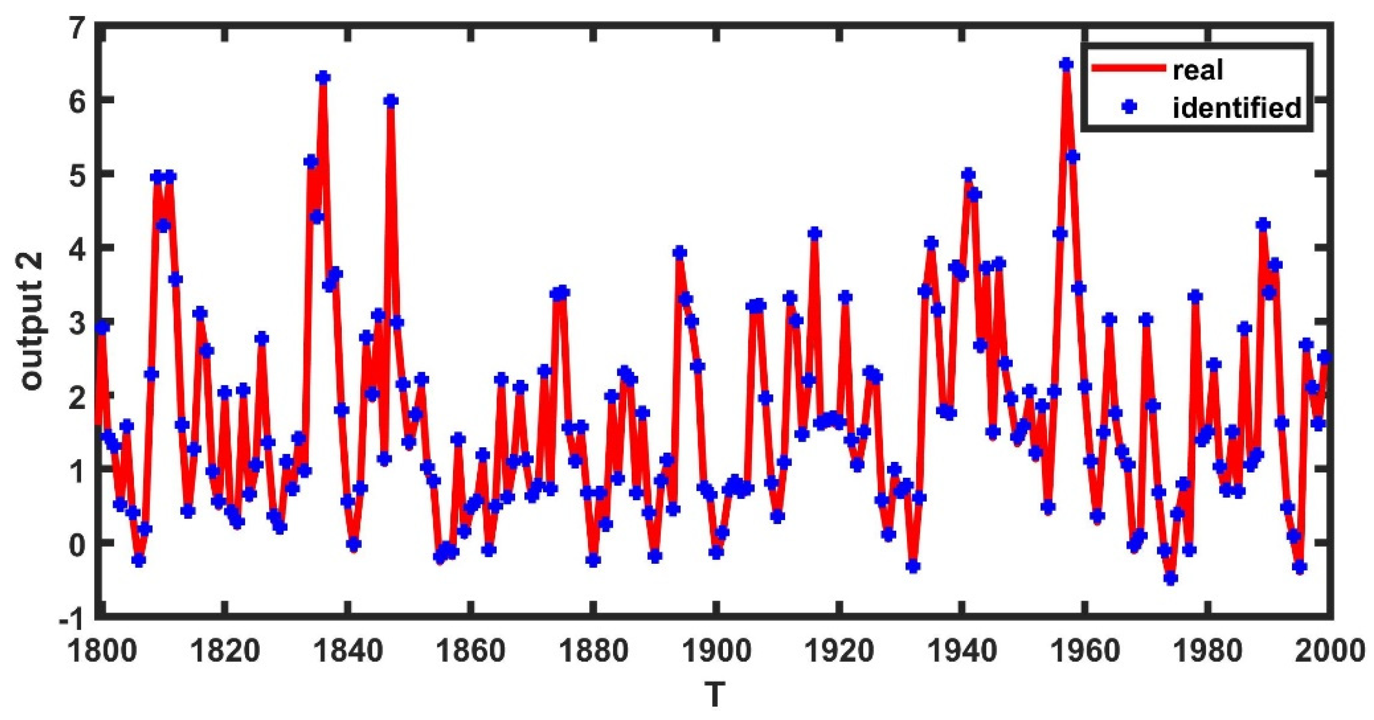
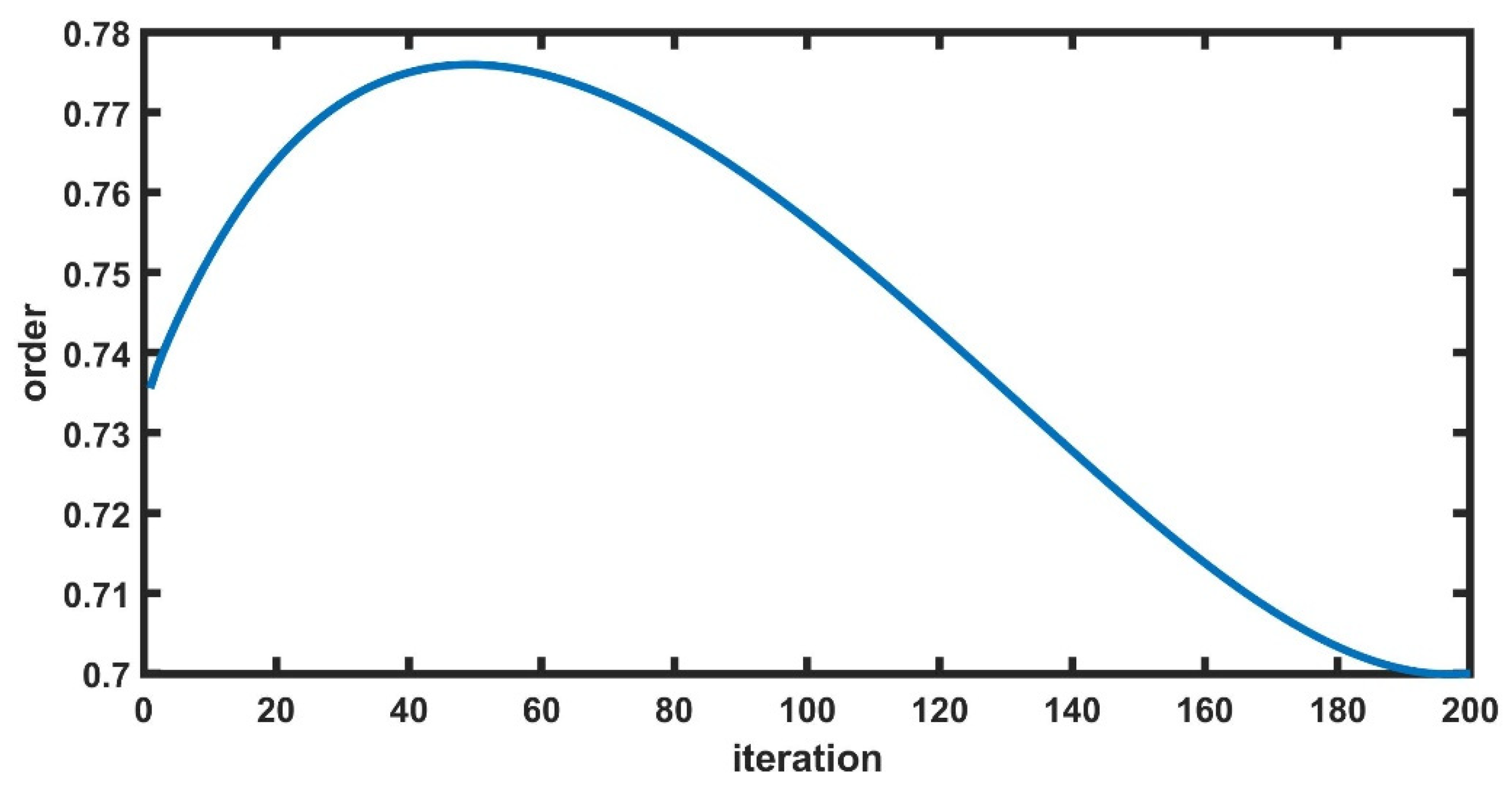
4.2. Example 2
5. Conclusions
Author Contributions
Funding
Institutional Review Board Statement
Informed Consent Statement
Data Availability Statement
Conflicts of Interest
References
- Billings, S.A.; Fakhouri, S.Y. Identification of systems containing linear dynamic and static nonlinear element. Automatica 1982, 18, 15–26. [Google Scholar] [CrossRef]
- Narendra, K.S.; Gallman, P.G. An Iterative Method for the Identification of Nonlinear Systems using the Hammerstein Model. IEEE Trans. Autom. Control 1966, AC11, 546–550. [Google Scholar] [CrossRef]
- Moghaddam, M.J.; Mojallali, H.; Teshnehlab, M. Recursive identification of multiple-input single-output fractional-order Hammerstein model with time delay. Appl. Soft Comput. 2018, 70, 486–500. [Google Scholar] [CrossRef]
- Chen, H.F. Strong consistency of recursive identification for Hammerstein systems with discontinuous piecewise-linear memoryless block. IEEE Trans. Autom. Control AC 2005, 50, 1612–1617. [Google Scholar] [CrossRef]
- Sznaier, M. Computational complexity analysis of set membership identification of Hammerstein and Wiener systems. Automatica 2009, 45, 701–705. [Google Scholar] [CrossRef]
- Kung, M.C.; Womack, B. Discrete time adaptive control of linear dynamic systems with a two-segment piecewise-linear asymmetric nonlinearity. IEEE Trans. Autom. Control 2003, 29, 170–172. [Google Scholar] [CrossRef]
- Mccannon, T.E.; Gallagher, N.C.; Minoo-Hamedani, D.; Wise, J.L. On the design of nonlinear discrete-time predictors. IEEE Trans. Inf. Theory 1982, 28, 366–371. [Google Scholar] [CrossRef]
- Jin, Q.; Wang, H.; Su, Q. A novel optimization algorithm for MIMO Hammerstein model identification under heavy-tailed noise. ISA Trans. 2018, 72, 77–91. [Google Scholar] [CrossRef] [PubMed]
- Jin, Q.; Xu, Z.; Cai, W. An Improved Whale Optimization Algorithm with Random Evolution and Special Reinforcement Dual-Operation Strategy Collaboration. Symmetry 2021, 13, 238. [Google Scholar] [CrossRef]
- Dong, S.; Yu, L.; Zhang, W.A. Robust extended recursive least squyares identification algorithm for Hammerstein systems with dynamic disturbances. Digit. Signal Process. 2020, 101, 102716. [Google Scholar] [CrossRef]
- Dhaifallah, M.A.; Westwick, D.T. Support Vector Machine Identification of Output Error Hammerstein Models. IFAC Proc. Vol. 2011, 44, 13948–13953. [Google Scholar] [CrossRef]
- Schlegel, M.; Čech, M. Fractal System Identification for Robust Control—The Moment Approach. In Proceedings of the 5th International Carpathian Control Conference, Zakopane, Poland, 25–28 May 2004. [Google Scholar]
- Torvik, P.J.; Bagley, R.L. On the Appearance of the Fractional Derivative in the Behavior of Real Materials. J. Appl. Mech. 1984, 51, 725–728. [Google Scholar] [CrossRef]
- Zhao, C.; Dingy, X. Closed-form solutions to fractional-order linear differential equations. Front. Electr. Electr. Eng. China 2008, 3, 214–217. [Google Scholar] [CrossRef]
- Chen, S.; Liu, F.; Turner, I. Numerical inversion of the fractional derivative index and surface thermal flux for an anomalous heat conduction model in a multi-layer medium. Appl. Math. Model. 2018, 59, 514–526. [Google Scholar] [CrossRef] [Green Version]
- Deng, J. Higher-order stochastic averaging for a SDOF fractional viscoelastic system under bounded noise excitation. J. Frankl. Inst. 2017, 354, 7917–7945. [Google Scholar] [CrossRef]
- Das, S. Functional Fractional Calculus; Springer: Berlin/Heidelberg, Germany, 2011; pp. 110–122. [Google Scholar]
- Table, M.A.; Béthoux, O.; Godoyb, E. Identification of a PEMFC fractional order model. Int. J. Hydrogen Energy 2017, 42, 1499–1509. [Google Scholar]
- Kumar, S.; Ghosh, A. Identification of fractional order model for a voltammetric E-tongue system. Measurement 2019, 150, 107064. [Google Scholar] [CrossRef]
- Zhang, Q.; Shang, Y.; Li, Y. A novel fractional variable-order equivalent circuit model and parameter identification of electric vehicle Li-ion batteries. ISA Trans. 2019, 97, 448–457. [Google Scholar] [CrossRef]
- Hammar, K.; Djamah, T.; Bettayeb, M. Fractional hammerstein system identification using particle swarm optimization. In Proceedings of the 2015 7th International Conference on Modelling, Identification and Control (ICMIC) 2015, Sousse, Tunisia, 18–20 December 2015; pp. 1–6. [Google Scholar]
- Hammar, K.; Djamah, T.; Bettayeb, M. Fractional Hammerstein system identification based on two decomposition principles. IFAC-PapersOnLine 2019, 52, 206–210. [Google Scholar] [CrossRef]
- Chetoui, M.; Aoun, m. Instrumental variables based methods for linear systems identification with fractional models in the EIV context. In Proceedings of the 2019 16th International Multi-Conference on Systems, Signals & Devices (SSD) 2019, Istanbul, Turkey, 21–24 March 2019; pp. 90–95. [Google Scholar]
- Wang, J.; Wei, Y.; Liu, T. Fully parametric identification for continuous time fractional order Hammerstein systems. J. Frankl. Inst. 2020, 357, 651–666. [Google Scholar] [CrossRef]
- Cui, R.; Wei, Y.; Chen, Y. An innovative parameter estimation for fractional-order systems in the presence of outliers. Nonlinear Dyn. 2017, 89, 453–463. [Google Scholar] [CrossRef]
- Tang, Y.; Liu, H.; Wang, W. Parameter identification of fractional order systems using block pulse functions. Signal Process. 2015, 107, 272–281. [Google Scholar] [CrossRef]
- Cui, R.; Wei, Y.; Cheng, S. An innovative parameter estimation for fractional order systems with impulse noise. Isa Trans. 2017, 120–129. [Google Scholar] [CrossRef] [PubMed]
- Zhao, Y.; Yan, L.; Chen, Y. Complete parametric identification of fractional order Hammerstein systems. In Proceedings of the ICFDA’14 International Conference on Fractional Differentiation and Its Applications 2014, Catania, Italy, 23–25 June 2014; pp. 1–6. [Google Scholar]
- Zeng, L.; Zhu, Z.; Shu, L. Subspace identification for fractional order Hammerstein systems based on instrumental variables. Int. J. Control Autom. Syst. 2012, 10, 947–953. [Google Scholar]
- Khanra, M.; Pal, J. Reduced Order Approximation of MIMO Fractional Order Systems. IEEE J. Emerg. Sel. Top. Circuits Syst. 2013, 3, 451–458. [Google Scholar] [CrossRef]
- Lakshmikantham, V.; Vatsala, A.S. Basic theory of fractional differential equations. Nonlinear Anal. Theory Methods Appl. 2008, 69, 2677–2682. [Google Scholar] [CrossRef]
- Chun, J.S.; Jung, H.K.; Hahn, S.Y. A study on comparison of optimization performances between immune algorithm and other heuristic algorithms. IEEE Trans Magn. 1998, 34, 297222975. [Google Scholar]
- Castro, L.N.; Castro, D.L.; Timmis, J. Artificial Immune Systems: A New Computational Intelligence Approach; Springer Science & Business Media: London, UK, 2002. [Google Scholar]
- Chen, X.L.; Li, J.Q.; Han, Y.Y. Improved artificial immune algorithm for the flexible job shop problem with transportation time. Meas. Control 2020, 53, 2111–2128. [Google Scholar] [CrossRef]
- Lu, L.; Guo, Z.; Wang, Z. Parameter Estimation for a Capacitive Coupling Communication Channel Within a Metal Cabinet Based on a Modified Artificial Immune Algorithm. IEEE Access 2021, 75683–75698. [Google Scholar] [CrossRef]
- Samigulina, G.; Samigulina, Z. Diagnostics of industrial equipment and faults prediction based on modified algorithms of artificial immune systems. J. Intell. Manuf. 2021. [Google Scholar] [CrossRef]
- Yu, T.; Xie, M.; Li, X. Quantitative method of damage degree of power system network attack based on improved artificial immune algorithm. In Proceedings of the ICAIIS 2021: 2021 2nd International Conference on Artificial Intelligence and Information Systems, Chongqing, China, 28–30 May 2021. [Google Scholar]
- Xu, Y.; Zhang, J. Regional Integrated Energy Site Layout Optimization Based on Improved Artificial Immune Algorithm. Energies 2020, 13, 4381. [Google Scholar] [CrossRef]
- Eker, E.; Kayri, M.; Ekinci, S. A New Fusion of ASO with SA Algorithm and Its Applications to MLP Training and DC Motor Speed Control. Arab. J. Sci. Eng. 2021, 46, 3889–3911. [Google Scholar] [CrossRef]
- Wu, G.; Mallipeddi, R.; Suganthan, P.N. Problem Definitions and Evaluation Criteria for the CEC 2017 Competition and Special Session on Constrained Single Objective Real-Parameter Optimization; Technical Report; Nanyang Technological University: Singapore, 2016. [Google Scholar]
- Heidari, A.A.; Mirjalili, S.; Faris, H.; Aljarah, H. Harris hawks optimization: Algorithm and applications. Future Gener. Comput. Syst. 2019, 97, 849–872. [Google Scholar] [CrossRef]
- Abualigah, L.; Yousri, D.; Elaziz, M.A. Matlab Code of Aquila Optimizer: A novel meta-heuristic optimization algorithm. Comput. Ind. Eng. 2021, 157, 107250. [Google Scholar] [CrossRef]
- Dzieliński, A.; Sierociuk, D. Stability of discrete fractional order state-space systems. IFAC Proc. Vol. 2006, 39, 505–510. [Google Scholar] [CrossRef]
- Ding, F.; Chen, H.; Li, M. Multi-innovation least squares identification methods based on the auxiliary model for MISO systems. Appl. Math. Comput. 2007, 187, 658–668. [Google Scholar] [CrossRef]
- Zhao, X.; Lin, Z.; Bo, F. Research on Automatic Generation Control with Wind Power Participation Based on Predictive Optimal 2-Degree-of-Freedom PID Strategy for Multi-area Interconnected Power System. Energies 2018, 11, 3325. [Google Scholar] [CrossRef] [Green Version]
- Ding, J.; Chen, J.; Lin, J. Particle filtering based parameter estimation for systems with output-error type model structures. J. Frankl. Inst. 2019, 356, 5521–5540. [Google Scholar] [CrossRef]
- Wang, L.; Liu, H.; Dai, L. Novel Method for Identifying Fault Location of Mixed Lines. Energies 2018, 11, 1529. [Google Scholar] [CrossRef] [Green Version]


| Name | Formula | Range | |
|---|---|---|---|
| Sphere | [−20, 20] | 0 | |
| Schwefel 1.2 | [−100, 100] | 0 | |
| Rosenbrock | [−30, 30] | 0 | |
| Step | [−100, 100] | 0 | |
| Ackley | [−40, 40] | 0 | |
| Generalized penalized 1 | [−50, 50] | 0 | |
| Generalized penalized 2 | [−50, 50] | 0 | |
| Shekel’s Foxholes | [−70, 70] | 1 | |
| Hybrid function 4 (N = 4) | [−100, 100] | 1400 | |
| Hybrid function 7 (N = 5) | [−100, 100] | 1700 | |
| Composition function 1 (N = 3) | [−100, 100] | 2100 | |
| Composition function 4 (N = 4) | [−100, 100] | 2400 |
| Algorithm | Parameter Settings |
|---|---|
| AIAGS | δ = 0.1, sv = 0.2 |
| AO | α = 0.5, δ = 0.5 |
| IA | α = 2, β = 1, δ = 0.2, pm = 0.7 |
| IAIA | α = 2, β = 1, δ = 0.613, pm = 0.7 |
| MAIA | δ = 0.8, pm = 0.8, cr = 0.8 |
| HHO | α = 0.5, δ = 0.5 |
| AIAGS | AO | IA | IAIA | MAIA | HHO | |
|---|---|---|---|---|---|---|
| F1 | ||||||
| worst | 0 | 2.86 × 10−71 | 0.000124 | 0.000145 | 0.030882 | 1.98 × 10−46 |
| best | 0 | 7.37 × 10−76 | 7.65 × 10⁻⁵ | 3.54 × 10⁻⁵ | 0.001683 | 2.62 × 10−58 |
| Avg | 0 | 5.74 × 10−72 | 9.86 × 10⁻⁵ | 7.71 × 10⁻⁵ | 0.012509 | 1.99 × 10−47 |
| Std | 0 | 1 × 10−71 | 1.46 × 10⁻⁵ | 3.28 × 10⁻⁵ | 0.009914 | 5.95 × 10−47 |
| F2 | ||||||
| worst | 0 | 2.82 × 10−56 | 0.006578 | 0.022761 | 16.07011 | 1.71 × 10−42 |
| best | 0 | 1.72 × 10−73 | 0.002606 | 0.013182 | 0.812125 | 1.15 × 10−51 |
| Avg | 0 | 2.82 × 10−57 | 0.003962 | 0.017273 | 4.565824 | 3.78 × 10−43 |
| Std | 0 | 8.93 × 10−57 | 0.001401 | 0.003087 | 4.947259 | 6.69 × 10−43 |
| F3 | ||||||
| worst | 6.39 × 10⁻⁷ | 0.001305 | 433.5283 | 696.2436 | 83.41411 | 0.008889 |
| Best | 5.5 × 10⁻⁹ | 5 × 10⁻⁶ | 0.99727 | 0.762353 | 4.4702 | 2.1 × 10⁻⁵ |
| Avg | 9.99 × 10⁻⁸ | 0.000319 | 80.76008 | 143.8289 | 29.75245 | 0.002238 |
| Std | 1.83 × 10⁻⁷ | 0.000424 | 143.8194 | 240.8117 | 30.68641 | 0.002581 |
| F4 | ||||||
| worst | 0 | 6.97 × 10⁻⁵ | 0.004139 | 0.00329 | 0.00329 | 9.33 × 10⁻⁵ |
| Best | 0 | 2.3 × 10⁻⁷ | 0.001612 | 0.00174 | 0.00174 | 7.93 × 10⁻¹⁰ |
| Avg | 0 | 1.87 × 10⁻⁵ | 0.003066 | 0.002567 | 0.002567 | 2.05 × 10⁻⁵ |
| Std | 0 | 2.32 × 10⁻⁵ | 0.00077 | 0.00053 | 0.00053 | 2.64 × 10⁻⁵ |
| F5 | ||||||
| worst | 8.88 × 10⁻¹⁶ | 8.88 × 10⁻¹⁶ | 4.663342 | 3.223428 | 1.019824 | 8.88 × 10⁻¹⁶ |
| Best | 8.88 × 10⁻¹⁶ | 8.88 × 10⁻¹⁶ | 0.017455 | 0.019081 | 0.137416 | 8.88 × 10⁻¹⁶ |
| Avg | 8.88 × 10⁻¹⁶ | 8.88 × 10⁻¹⁶ | 1.139553 | 0.342006 | 0.437464 | 8.88 × 10⁻¹⁶ |
| Std | 0 | 0 | 1.617355 | 1.012431 | 0.323219 | 0 |
| F6 | ||||||
| worst | 4.71 × 10⁻³² | 3.84 × 10⁻⁵ | 4.772913 | 6.250579 | 0.005788 | 2.07 × 10⁻⁵ |
| Best | 4.71 × 10⁻³² | 7.83 × 10⁻⁸ | 1.16 × 10⁻⁵ | 0.335882 | 0.000107 | 1.56 × 10⁻⁷ |
| Avg | 4.71 × 10⁻³² | 7.48 × 10⁻⁶ | 1.984778 | 3.781554 | 0.001743 | 6.34 × 10⁻⁶ |
| Std | 0 | 1.16 × 10⁻⁵ | 1.830602 | 2.512286 | 0.002048 | 6.86 × 10⁻⁶ |
| F7 | ||||||
| worst | 1.35 × 10⁻³² | 0.000281 | 0.000101 | 8.19 × 10⁻⁵ | 0.039677 | 0.000501 |
| best | 1.35 × 10⁻³² | 1.31 × 10⁻⁶ | 5.21 × 10⁻⁵ | 3.87 × 10⁻⁵ | 0.002672 | 1.18 × 10⁻⁷ |
| Avg | 1.35 × 10⁻³² | 4.25 × 10⁻⁵ | 8.01 × 10⁻⁵ | 5.89 × 10⁻⁵ | 0.017996 | 8.5 × 10⁻⁵ |
| Std | 2.88 × 10−48 | 8.69 × 10⁻⁵ | 1.55 × 10⁻⁵ | 1.58 × 10⁻⁵ | 0.01293 | 0.000143 |
| F8 | ||||||
| worst | 0.998004 | 2.982105 | 1.992031 | 0.998004 | 0.999027 | 1.992031 |
| best | 0.998004 | 0.998004 | 0.998004 | 0.998004 | 0.998004 | 0.998004 |
| Avg | 0.998004 | 1.593234 | 1.166875 | 0.998004 | 0.998107 | 1.196819 |
| Std | 2.34 × 10⁻¹⁶ | 0.958412 | 0.362935 | 2.01 × 10⁻¹⁵ | 0.000323 | 0.397606 |
| F9 | ||||||
| worst | 1528.366 | 5142.015 | 2215.496 | 2302.871 | 5755.439 | 4349.2 |
| best | 1472.889 | 1557.776 | 1443.205 | 1428.962 | 1488.148 | 1450.039 |
| Avg | 1503.786 | 2462.484 | 1580.193 | 1655.434 | 2510.73 | 1833.8 |
| Std | 19.26844 | 978.4552 | 223.2629 | 287.2931 | 1264.939 | 843.7423 |
| F10 | ||||||
| worst | 1794.68 | 1838.131 | 1763.443 | 1782.14 | 2200.955 | 1840.59 |
| Best | 1744.138 | 1731.296 | 1722.813 | 1725.397 | 1766.414 | 1744.772 |
| Avg | 1774.579 | 1781.842 | 1738.947 | 1748.674 | 1898.936 | 1781.998 |
| Std | 17.10128 | 32.03933 | 10.8574 | 22.15373 | 122.3724 | 30.2191 |
| F11 | ||||||
| worst | 2260.104 | 2338.993 | 2264.487 | 2288.434 | 2319.733 | 2388.341 |
| Best | 2209.787 | 2204.09 | 2200.005 | 2200.003 | 2201.822 | 2205.34 |
| Avg | 2236.802 | 2272.26 | 2211.444 | 2211.249 | 2265.511 | 2272.888 |
| Std | 18.17673 | 56.04231 | 18.0651 | 25.8142 | 44.29724 | 71.44948 |
| F12 | ||||||
| worst | 2717.367 | 2778.692 | 2772.984 | 2762.261 | 2824.593 | 2857.503 |
| Best | 2521.748 | 2746.416 | 2500.074 | 2500.073 | 2505.906 | 2770.847 |
| Avg | 2626.946 | 2767.838 | 2669.676 | 2629.372 | 2710.07 | 2799.953 |
| Std | 61.88762 | 9.524766 | 114.739 | 111.2591 | 104.6337 | 28.32715 |
| Method (and AMRLS) | ||||||||||||||||
|---|---|---|---|---|---|---|---|---|---|---|---|---|---|---|---|---|
| AIAGS | 5.127 | 3.120 | 3.976 | 2.959 | 6.118 | 2.017 | 3.996 | 4.970 | 0.501 | 0.289 | 0.095 | 0.400 | 0.200 | 0.100 | 0.299 | 0.333 |
| AO | 4.619 | 3.325 | 3.887 | 3.465 | 5.377 | 1.760 | 4.196 | 5.272 | 0.509 | 0.297 | 0.098 | 0.404 | 0.198 | 0.098 | 0.275 | 0.391 |
| HHO | 4.641 | 3.329 | 3.882 | 3.448 | 5.289 | 1.757 | 4.152 | 5.283 | 0.508 | 0.296 | 0.097 | 0.404 | 0.198 | 0.099 | 0.278 | 0.382 |
| Method (and AMRLS) | AIAGS | AO | HHO |
|---|---|---|---|
| RQE | 0.1360 | 0.2931 | 0.2987 |
| MSE | 0.0144 | 0.0944 | 0.1019 |
| Method (and AMRLS) | α | ||||||||||||||||||
|---|---|---|---|---|---|---|---|---|---|---|---|---|---|---|---|---|---|---|---|
| AIAGS | 2.002 | 1.501 | 1.297 | 5.033 | 1.703 | 1.915 | 2.164 | 2.215 | 1.766 | 1.675 | 1.564 | 1.029 | 0.504 | 0.191 | 0.095 | 0.385 | 0.293 | 0.101 | 0.700 |
| AO | 2.946 | 1.453 | 1.174 | 5.642 | 1.127 | 1.832 | 2.459 | 2.544 | 0.733 | 4.680 | 1.626 | 1.122 | 0.483 | 0.188 | 0.100 | 0.347 | 0.290 | 0.106 | 0.582 |
| HHO | 3.182 | 1.42 | 1.197 | 5.697 | 1.004 | 1.808 | 2.463 | 2.605 | 0.691 | 4.962 | 1.631 | 1.132 | 0.482 | 0.188 | 0.100 | 0.344 | 0.288 | 0.106 | 0.570 |
| Method (and AMRLS) | AIAGS | AO | HHO |
|---|---|---|---|
| RQE | 0.1819 | 0.6579 | 0.6935 |
| MSE | 0.0351 | 0.5133 | 0.6626 |
Publisher’s Note: MDPI stays neutral with regard to jurisdictional claims in published maps and institutional affiliations. |
© 2022 by the authors. Licensee MDPI, Basel, Switzerland. This article is an open access article distributed under the terms and conditions of the Creative Commons Attribution (CC BY) license (https://creativecommons.org/licenses/by/4.0/).
Share and Cite
Jin, Q.; Wang, B.; Wang, Z. Recursive Identification for MIMO Fractional-Order Hammerstein Model Based on AIAGS. Mathematics 2022, 10, 212. https://doi.org/10.3390/math10020212
Jin Q, Wang B, Wang Z. Recursive Identification for MIMO Fractional-Order Hammerstein Model Based on AIAGS. Mathematics. 2022; 10(2):212. https://doi.org/10.3390/math10020212
Chicago/Turabian StyleJin, Qibing, Bin Wang, and Zeyu Wang. 2022. "Recursive Identification for MIMO Fractional-Order Hammerstein Model Based on AIAGS" Mathematics 10, no. 2: 212. https://doi.org/10.3390/math10020212