1. Introduction
The field of Artificial Intelligence (AI) is usually divided into two opposing points of view: on the one hand, we have the Symbolic AI, which focuses on a symbolic representation of the world and then uses logic and search to solve problems, and on the other hand, we have the subsymbolic AI that does not use explicit high-level symbols and relies on mathematical equations to solve problems. Inside the subsymbolic approach, we can find the connectionist models, that aim to build networks of simple interconnected units that aim to simulate the functioning of the human brain [
1]. The subsymbolic field includes the Machine Learning (ML) disciplines, which focus on constructing computer systems that automatically improve through experience. It also includes the study of the fundamental statistical, computational, information and theoretic laws behind these learning systems [
2].
The field of Quantum Computing has proven to be better than classical computers at solving certain types of problems. For example: algebraic computational problems, such as the Shor algorithm [
3]; optimization and simulation tasks, such as simulated annealing; database search, such as the Grover’s search algorithm [
4]; or sampling problems, such as the Markov Chain Monte Carlo methods. In general, we can say that the advantage that quantum computation offers is the exploitation of an exponentially large quantum state space through controllable entanglement and interference [
5].
Since ML models and applications deal with massive parallel processing of high-dimensional data, it seems obvious that quantum computers can be an advantage when designing ML algorithms. Thus, a new field called Quantum Machine Learning (QML) has emerged, where quantum algorithms have been defined for ML tasks that exhibit quantum speedups [
6,
7,
8,
9].
However, the field of symbolic AI seems not to have benefited greatly from the existence of quantum computers. There are some suggestions: for example, since there are algorithms developed to solve pattern matching problems, that is, the search for certain types of patterns in certain search spaces (e.g., the search for substrings in long text sources such as [
10,
11]) that are inspired in Grover’s search algorithm [
4]; it has been suggested to use quantum pattern matching to perform pattern matching of rule-based systems [
12].
A more promising line for incorporating quantum computation into symbolic AI is to use the probabilistic nature of quantum systems to represent imprecision and uncertainty. Reasoning with inaccurate knowledge is one of the fundamental problems of symbolic AI [
13]. Broadly speaking, we can consider that the origin of inaccurate knowledge is related to one or more of the following causes [
14]: (1) the available information is incomplete, (2) the available information is incorrect, (3) the information we use is inaccurate, (4) the real world is not deterministic, (5) the lack of agreement between experts in the same field is frequent, and (6) the knowledge model contains inaccurate information.
One of the first successful models to deal with uncertainty was the Certainty Factors model proposed by Shortliffe and Buchanan (S.B.) [
15] that shook the foundations of the, at that moment, incipient world of artificial intelligence. The Shortliffe and Buchanan model of certainty factors is ad hoc in nature and therefore lacks a strong theoretical basis. However, this model was immediately accepted due to its easy understanding and the quality of the results obtained after its application. In any case, it appears that, despite its ad hoc nature, probabilities are in the core of this certainty factors [
16].
Later approaches to model inexact knowledge include fuzzy models [
17] based on fuzzy sets, the evidential theory of Dempster and Shafer [
18], and the Bayesian networks (or belief networks) [
19] that combine graph theory and probability theory.
Although the certainty factors model is independent of the technology, the real fact is that, at present, we can start thinking on taking advantage of quantum systems and consider specific applications of quantum computing (Q.C.), since we currently are in the noisy intermediate-scale quantum (NISQ) era [
20]. In this context, the question is [
21]: Could we use actual quantum computing (which is intrinsically probabilistic) to investigate the probabilistic nature of certainty factors for reasoning with inaccurate knowledge?
Although this paper is strongly based on what we have already published in [
13], the major novelty of this work is to show how a well-established method [
15] for dealing with inaccurate knowledge can be implemented and studied from a quantum viewpoint.
In this context, a specific use case was built: an inferential network for testing the behaviour of the certainty factors approach in a quantum environment. After the design and execution of the experiments, the corresponding analysis of the obtained results is performed in three different scenarios: (1) inaccuracy in declarative knowledge, or imprecision, (2) inaccuracy in procedural knowledge, or uncertainty, and (3) inaccuracy in both declarative and procedural knowledge.
We hope this paper paves the way for future quantum implementations of well-established, traditional methods for handling inaccurate knowledge.
2. The Certainty Factors Model
The basic ideas of the certainty factors model can be summarized in the following points [
15]: (a) given a hypothesis that is being considered, the evidential strength of a statement should be represented by two different measures: the Measure of Increasing Belief,
, and the Measure of Increasing Disbelief,
; (b)
and
are dynamic indexes that represent increments associated with new evidence; (c) if
h is a hypothesis, and
e is an evidence, the same evidence
e cannot simultaneously increase belief and disbelief in
h; (d)
represents an increase in belief in the hypothesis
h given the new evidence
e; and (e)
represents an increase in disbelief in the hypothesis
h given the new evidence
e.
Now, let be the a priori probability of h and let be the probability of h after e. Note that is a probability, and is a conditional probability. With these assumptions, we can identify the following cases:
If
, then there is an increase in the probability of the hypothesis
h after
e. In this case:
,
, and
is defined as follows:
According to this expression, represents a relative increase in the likelihood of the hypothesis h after evidence e.
If
, then there is a decrease in the probability of the hypothesis
h after
e. In this case:
,
, and
is defined as follows:
According to this expression, represents a relative increase in the negation of the likelihood of the hypothesis h after evidence e.
If
, then either the new evidence
e is independent of the hypothesis
h or there is no knowledge about an eventual causal relationship between
h and
e. In this case:
In addition to
and
, Shortliffe and Buchanan define a third index, the Certainty Factor,
, which combines the two previous measures according to the expression:
The above formula is a formal equation since the same evidence cannot simultaneously increase belief and disbelief about the same hypothesis. Shortliffe and Buchanan proposed this certainty factor to facilitate the comparison between evidential strengths of alternative hypotheses related with the same evidence. According to their definitions, the ranges of each measure are:
Since all these indexes are based on probabilities, one could expect that they would behave as probabilities, but this could be not necessarily true.
According to Shortliffe and Buchanan, one of the weakest points of probabilistic models is the fact that the same evidence supports, simultaneously, a given hypothesis and its negation. This is a consequence of the mathematical consistency of probabilistic models, which forces that:
Following the arguments of Shortliffe and Buchanan, the certainty factors are not complementary to the unit as probabilities do. In fact,
. Assume that
—the same result is obtained if we consider that
—then:
Going a little bit deeper, the following question arises: how should an expert handle the certainty factors? For the specific case of a single piece of evidence, the answer is clear, as shown in these scenarios: (a) the expert indicates a value greater than zero and less than or equal to one, if the evidence in question supports the hypothesis, (b) the expert indicates a value less than zero but greater than or equal to minus one, if the evidence in question goes against the hypothesis, and (c) the expert indicates a value equal to zero, if he or she considers that the evidence found is independent of the considered hypothesis.
Another issue appears when there are several independent pieces of evidence pointing to the same hypothesis. In this case, we are talking about the combination of different pieces of evidence that are related to the same hypothesis. We can formulate this situation in the following terms: assume we have a set of rules, all of them with the same conclusion, each of them weighted with a different certainty factor. In addition, assume that
is all the evidence we have. What is the resulting certainty factor for the hypothesis
h given all the evidence
E? That is, what is the value of
?
In this case, each evidence
affects, in a different manner, to the veracity of the hypothesis under consideration. The problem is to find an adequate formulation that allows us to evaluate:
Shortliffe and Buchanan propose the following approach for the combination of two pieces of evidence that refer to the same hypothesis. The formulation in terms of certainty factors is as follows:
If
and
, then:
If
and
, then:
If
, then:
This way of combining evidence referring to the same hypothesis is associative, and when there are more than just two pieces of evidence, the combination of the different pieces of evidence can be considered in any order without affecting the final result.
Now, suppose the following inferential circuit:
How do we calculate
? We now face a problem of propagation of uncertainty. To solve it, Shortliffe and Buchanan propose the following equation:
This approach refers exclusively to the propagation of pure uncertainty, but it can also happen that input data are imprecise. There is a subtle difference between imprecision and uncertainty. Thus, while imprecision is a property associated with declarative knowledge (and therefore static), uncertainty is related to the evidential strength of causal relationships. For example: what should we conclude about
h, if instead of having
we have
, where
looks like
but is not exactly
? In this context, Shortliffe and Buchanan propose a formulation that treats imprecision as uncertainty. To do this, they modify the previous inferential circuit (Equation (
18)) as follows:
Now, in order to calculate
, the inaccurate knowledge—taking into account that
is the imprecision associated to
—is propagated as follows:
A final aspect related to the propagation of inaccurate knowledge is related to the logical combination of evidence. In production systems, rule antecedent clauses are usually nested through the logical operators {AND, OR, NOT}. In this context, Shortliffe and Buchanan propose the use of the minimum to evaluate the logical clause AND and the maximum to evaluate the logical clause OR.
As an example, consider the following rule, with the AND operator represented by the ∧ symbol and the OR operator represented by the ∨ symbol:
The antecedent of this rule is
. However, in a real problem, we usually have imprecise evidences
rather than categorical evidences
e. Therefore, the evidence we have is
, which is the evidence that modifies the antecedent of the rule. In this case, our problem is to find
:
This is the whole formulation of Shortliffe and Buchanan Certainty Factors Model, which serves as a basis for our work.
We chose this model to base this work for several reasons: (1) historically, the proposal of Shortliffe and Buchanan has had a great impact in the field of inaccurate reasoning; thus, we consider it a good starting point for our work on a quantum implementation of inaccurate reasoning, since we aim to model imprecision and uncertainty; (2) while the certainty factors model is not explicitly probabilistic, it is based on probabilities, and therefore we consider it interesting to study how this classical model compares to a quantum approach and its probabilistic nature; and (3) although it is not as popular as it was, there is still relevant work on certainty factors, such as [
22,
23,
24,
25].
To this we want to add, as is more thoroughly explained in [
26], that there exists a correlation between certainty factors and probabilities, which can lead to similarities with Bayesian belief-networks models, since both apply similar concepts. In this paper, certainty factors are just the employed model to compare and analyse the results obtained.
3. An Overview of Quantum Computing
In Quantum Computing, the information unit is the qubit. The qubit is a vector of a Hilbert space represented, in the Dirac notation, by a column matrix (Equation (
24)) in such a way that a bit 0 corresponds to a ket 0 and a bit 1 corresponds to a ket 1 [
27].
However, quantum systems can be in coherent superposition, which means that a quantum system can be simultaneously in the states ket 0 and ket 1. To describe this peculiarity, we need a state function,
, that verifies the following restrictions [
28]:
Note that the 1-qubit is built from the parameters and , which are the amplitudes of the state function. In addition, note that and are defined as complex numbers, which means that they have phase information, which allows one to perform rotations. This aspect is treated later when we implement inaccurate knowledge.
A direct consequence of Heisenberg’s indeterminacy principle [
29] is that when we observe (or measure) a given qubit in superposition, said qubit loses its quantum properties and collapses, irreversibly, in classical bits with a given probability.
A big difference between classical computing and quantum computing is related to the nature of logical gates. While quantum gates are bijective because they are unitary transformations, logical gates in general are not [
30]. The most important consequence of this property of quantum gates is that quantum states cannot be copied [
27]. Unlike conventional logic gates, which can operate from n-bits to m-bits, quantum gates must operate from n-qubits to n-qubits, and they are reversible. The reversibility of quantum gates is a consequence of the unitary nature of the corresponding operators. Each quantum gate of n-qubits can be represented by a unitary matrix of dimension
, where the transformation performed by the quantum gate is accomplished by its associated matrix operator. Taking into account the description of the transformation that a quantum gate performs on the elements of the basis space, the unitary matrix associated with it is obtained from the following procedure [
31]:
The rows of the matrix correspond to the basis vectors of the input;
The columns of the matrix correspond to the basis vectors of the output;.
The position of the matrix corresponds to the coefficient of the j basis vector output in relation to the i basis vector input.
Quantum gates that operate on a single qubit or 1-qubit systems (one input qubit and one output qubit) have associated
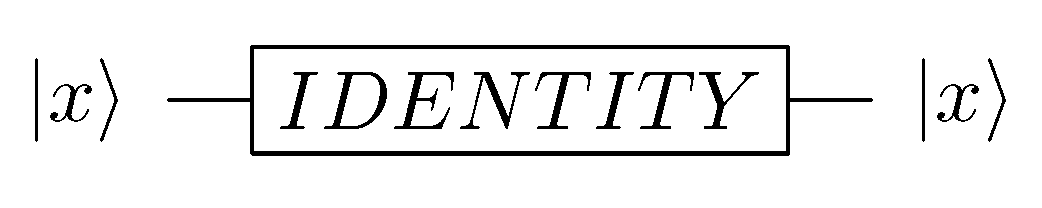
matrices. We now see how we can operate with some of these gates. We start with the identity gate,
I (
Figure 1), which, although its behaviour does not modify the state of the input qubit, serves to illustrate the procedure for constructing the associated unitary matrix.
Table 1 represents the truth table of the
I gate, and
Table 2 illustrates the associated unitary matrix of the
I operation.
The behaviour of the unitary matrix of the
I gate is as follows:
Similar to the identity gate
I is the negation gate,
N, usually described in quantum computing as the
X gate, which is as follows:
Finally, the Hadamard gate,
H, transforms a 1-qubit into a superposition of the elements of the basis
. The description and transformations that Hadamard’s gate performs are illustrated below:
Tensor products are used to build more complex systems of qubits. For example, we can build 2-qubit systems from the tensor product two 1-qubit systems. A 2-qubit system
is constructed as
. Therefore, if we consider the vectors of the basis for 1-qubit
, it follows that:
Therefore, the vectors of the basis for 2-qubit systems are , and the matrices that perform unitary transformations in 2-qubit systems must be matrices of dimension . Similarly, the vectors of the basis for 3-qubit systems are , and the matrices that perform unitary transformations in 3-qubit systems must be matrices of dimension .
In the context of 2-qubit systems, we mention the
gate (
-
), that negates the second qubit if the first qubit is |1〉.
Table 3 represents the truth table of the
gate, and
Table 4 illustrates the associated unitary matrix of the
operation. Clearly, the
of a
gate can be interpreted as the output of an
gate with inputs
and
; however, the device is not the same since the gate
generates two outputs instead of one.
Finally, in the context of 3-qubit systems, we mention the
gate (
-
-
, or Toffoli gate), that negates the third qubit when the first qubit is |1〉 and second qubit is |1〉.
Table 5 illustrates the associated unitary matrix of the
operation.
An interesting question is that with the quantum gates N, , and we can reproduce, in a probabilistic way, the behaviour of any conventional logical gate. If we also want to explore all the possibilities, we have to use H gates to set the state of the system in coherent superposition.
The simulation of conventional logical gates in a quantum environment can be performed through quantum circuits. Quantum circuits consist of quantum lines and quantum operations to perform the calculations, and conventional lines where the output qubits collapse after being measured. Following these lines, we illustrate some particular examples:
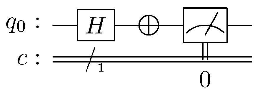
Quantum simulation of the classical NOT gate:
Figure 2 illustrates the quantum circuit for simulating a classical NOT gate, in which only one quantum line
is necessary to perform the calculations and only one conventional line
is necessary to record the result of the measurements. Gate
H places the system in a state of superposition, and gate ⨁ is a quantum NOT.
After the measurement, we have close to 50% of bits 0 and close to 50% of bits 1, which is what we expected.
Figure 3 shows the outputs obtained after running the program 1000 times in the IBM quantum simulator [
32].
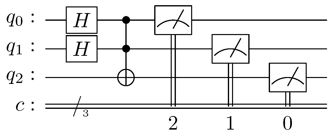
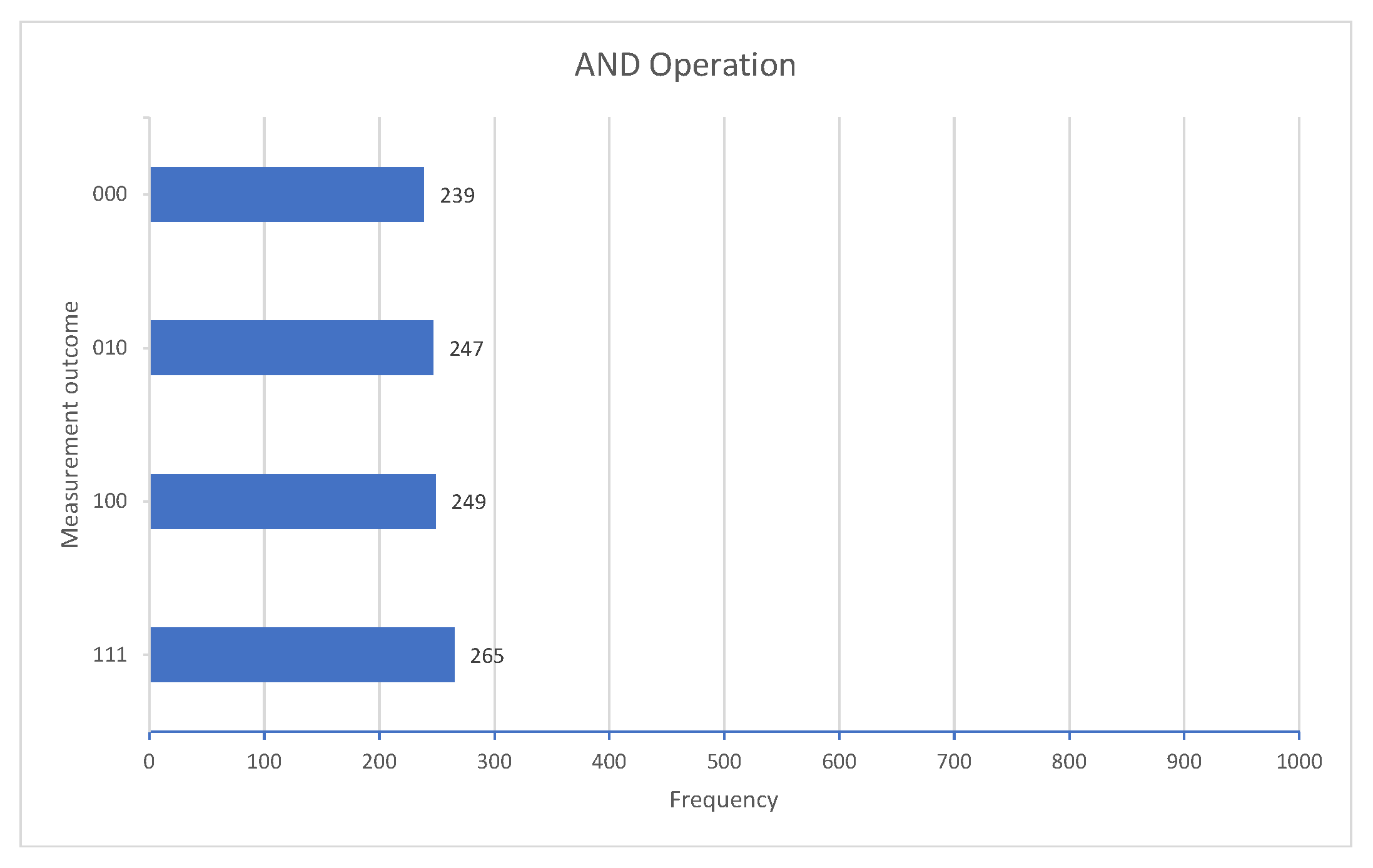
Quantum simulation of the AND gate:
Figure 4 illustrates the quantum circuit for simulating a classical AND gate, in which three quantum lines are necessary to perform the calculations, and only one conventional line is necessary to record the result of the operations. In this case, we measure the three qubits in order to illustrate the inputs and the outputs of the gate, where
is the result, and
and
are the inputs. Gates
H place the system in a state of superposition, and gate
is a quantum AND.
After the measurement, we have close to 25% for each of the possible outcomes, which is what we expected.
Figure 5 shows the outputs obtained after running the program 1000 times in the IBM quantum simulator [
32].
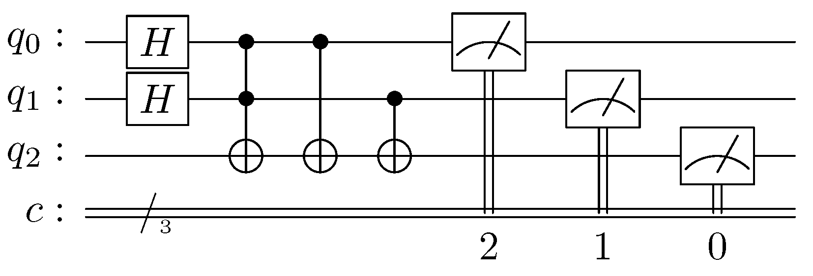
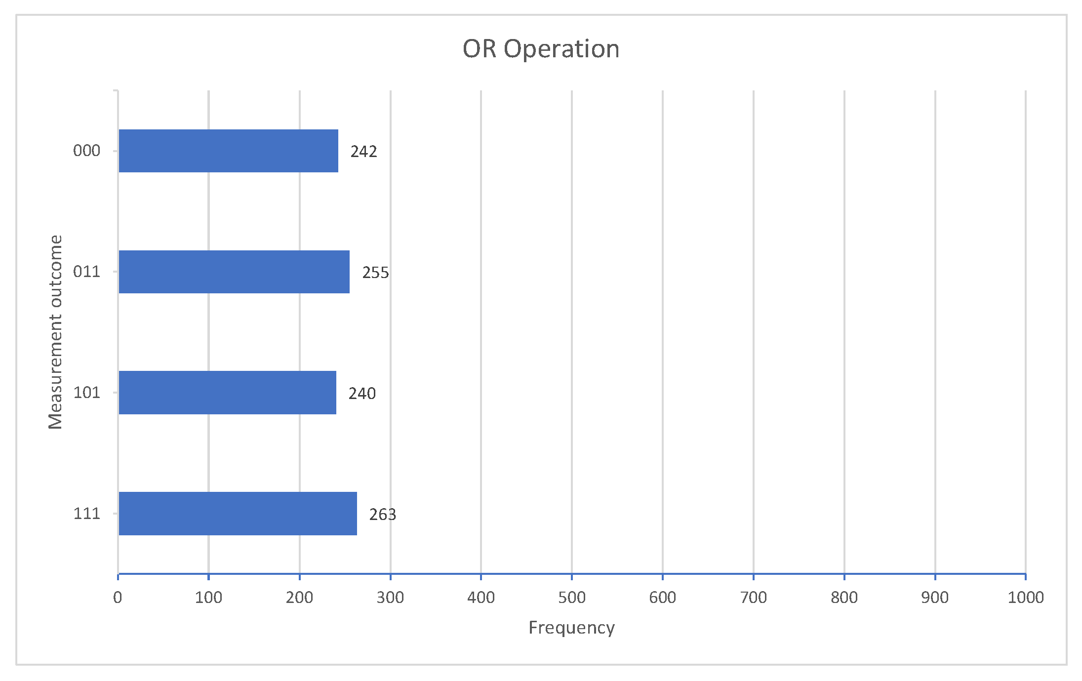
Quantum simulation of the OR gate:
Figure 6 illustrates the quantum circuit for simulating a classical OR gate, in which three quantum lines are necessary to perform the calculations, and only one conventional line is necessary to record the result of the operations. In this case, we measure the three qubits in order to illustrate the inputs and the outputs of the gate, where
is the result, and
and
are the inputs. Gates
H place the system in a state of superposition, and the set of gates
,
, and
is a quantum OR.
After the measurement, we have close to 25% for each of the possible outcomes, which is what we expected.
Figure 7 shows the outputs obtained after running the program 1000 times in the IBM quantum simulator [
32].
These examples are used in the next section to illustrate the implementation of the Certainty Factors Model for dealing with inaccurate knowledge in a quantum environment.
Before delving into that implementation, we want to clarify that this work does not look for quantum speedups for the time being. The focus of this work is to model imprecision and uncertainty by the means of quantum computing and see if we find a coherent and consistent model, which are compared to the classical approach of certainty factors.
This work is only theoretical still, and we will work on practical applications that will allow us to analyse whether this approach provides an improvement or not in comparison to its classical counterpart.
4. Correlating Certainty Factors with a Quantum Environment
In a previous paper [
13], we defined a general-purpose method for dealing with inaccuracy in quantum rule-based systems. Quantum rule-based systems are defined as quantum circuits that implement knowledge in the form of production rules. This permits to investigate the a priori probability given rules and facts, assuming that rules are true (
) and facts are true (
). In that case, inaccuracy comes from the propagation of the knowledge through the inferential network. A big difference between the original article and the procedure we are going to present is that, according to the model of Shortliffe and Buchanan, both declarative knowledge and procedural knowledge can be inaccurate; so apart from the inaccuracy introduced by the inferential network itself, we should be able to analyse the effects of imprecision and uncertainty in the behaviour of a well-established inaccurate knowledge management model.
4.1. A Classical Example
Assume the following set of rules {R1, R2, R3} and the following set of facts {A, B, C, D, E}, such that for each rule there is a and for each fact there is a . The specific rules are:
Note that in this case there is neither uncertainty (since rules are categorically true or categorically false) nor imprecision (since facts are categorically true or categorically false). However, inaccuracy appears spontaneously when propagating actual knowledge through the inferential network, and this inaccuracy is the a priori probability that we can expect given all possible cases that can be defined if H is our target.
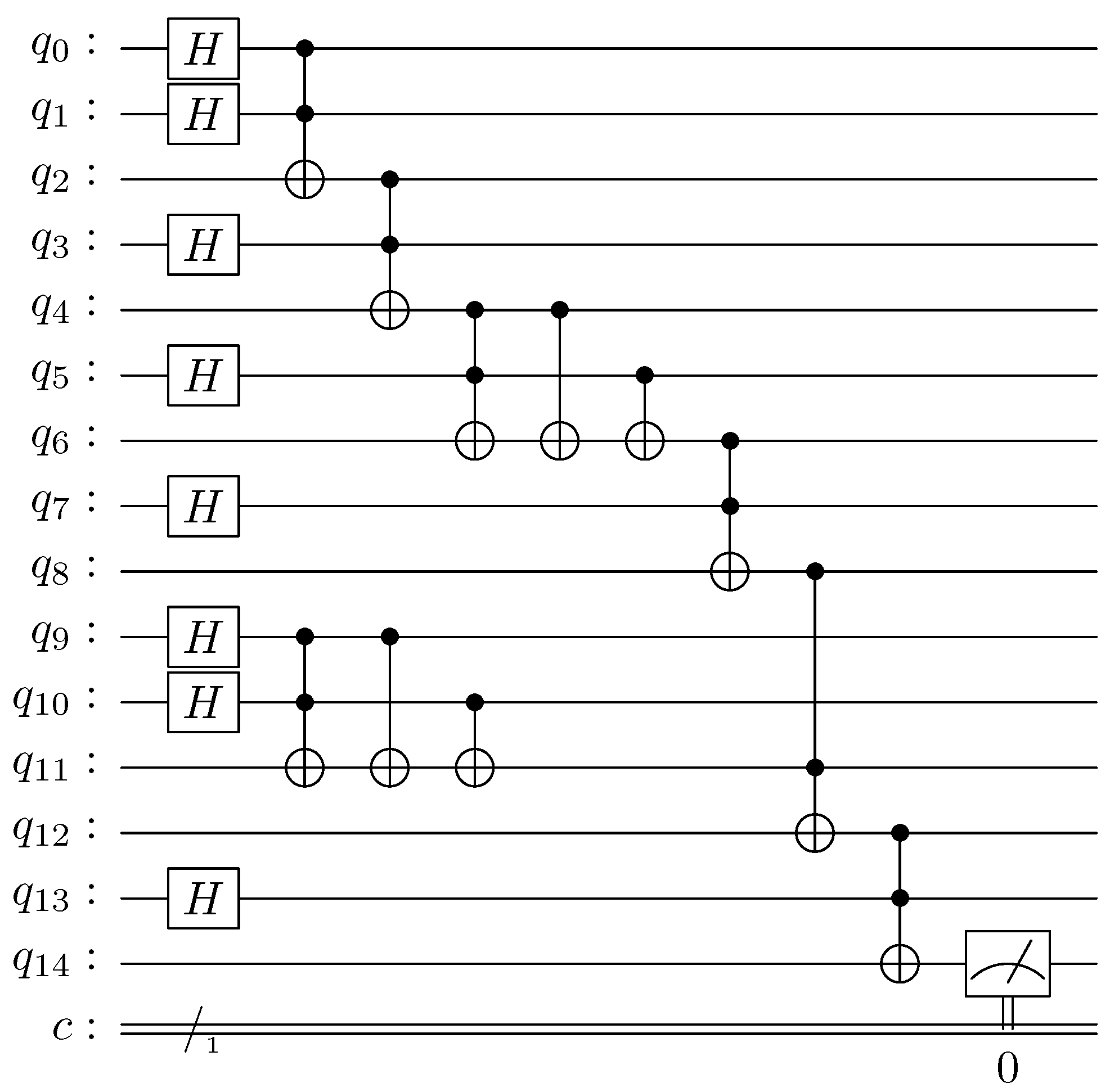
Figure 8 illustrates the classical inferential circuit that can be built from the abovementioned rules and facts.
The classical application of the Certainty Factors Model for investigating the a priori probability of hypothesis
H yields to the following results:
Given that
X,
Y, and
H are obtained through propagation, and in order to obtain the a priori probability of
H, we only need to set the values
or 1 for the facts A, B, C, D, and E, which implies the need to investigate
possibilities. The same applies for the rules R1, R2, and R3, which implies to investigate
possibilities. This results in a total of
cases to study. When performing this, the following results were obtained:
As previously mentioned, we can design a quantum circuit to resolve the same problem as above.
Figure 9 illustrates the quantum inferential circuit equivalent to the classical inferential circuit shown in
Figure 8.
Note that the architecture of
Figure 9 is a quantum representation of an intelligent rule-based system, by means of which we can conclude something about the hypothesis
H. In any case—since we work in superposition (
H gates)—the results are probabilistic. In fact, if we run this program 1000 times on the IBM quantum simulator [
32], we obtain the following results:
These results were obtained considering that the facts are categorically true or categorically false; therefore, there is no imprecision. Furthermore, we have not considered uncertainty in causal relationships.
Table 6 shows comparative results obtained with the classical approach and the quantum approach.
As expected, results of
Table 6 show strong agreement between the behaviour of both classical and quantum models.
4.2. Introducing Quantum Inaccuracy
The next step is to define a quantum method for dealing with imprecision in facts and with uncertainty in rules, in order to evaluate the inaccuracy of the hypothesis H in a real situation.
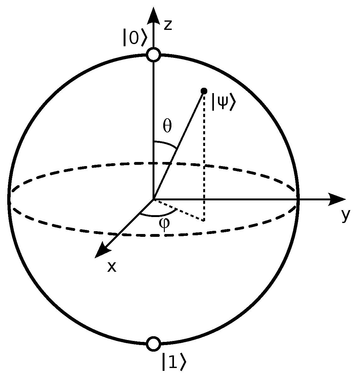
On the one hand, to define a general procedure capable of representing any degree of inaccuracy, it would be convenient to have a single quantum gate that, considering all the restrictions imposed by quantum mechanics, brings us closer to the world of analogic information. Our proposal starts with the Bloch sphere (
Figure 10), which, in quantum mechanics, is a geometric representation of the pure state space of a two-level quantum system [
33].
On the other hand, we already mentioned that quantum transformations are carried on by the means of unitary matrices that must be hermitian. Therefore, we assume that inaccuracy can be obtained from a unitary matrix that operates on a specific state of the quantum system. In this context, we introduce matrix
, defined as follows:
This matrix is clearly hermitic and unitary, since
. The input angle
ranges from values between 0 and
, so that, when the state of the system has an associated value of
, the statement is completely false, and when
, the statement is completely true. There is a direct correlation between the angle
and the angle
of the Bloch sphere (Equation (
40)); therefore, the angle
is no more than a rotation along the
Z axis.
Note that when or , there is not inaccuracy, since we have pure qubital states. In any other case, there is inaccuracy in the state function. According to this:
state is 0 → the associated statement is false;
state is 1 → the associated declaration is true;
state is in superposition → we are in a situation of coherent superposition, and the associated statement is neither true nor false, or—in an equivalent way—it is true and false simultaneously.
Finally, we need to establish the relationship between angle
and the certainty factors. First, we must normalise the certainty factors so that they range from 0 to 1 rather than from
to 1. For this, we propose the following equation:
With the normalized certainty factors, the relationship between CFs and angle
is as follows:
With this approach, we model the inaccurate knowledge in quantum rule-based systems, in which certainty factors are normalized.
5. Experimentation and Results
With the above ideas in mind, let us go back to the quantum inferential circuit of
Figure 9. This inferential circuit is used to model: (a) imprecision, (b) uncertainty, and (c) both imprecision and uncertainty simultaneously.
In the following subsections, we show each of the experiments and their results (S.B. for the Shortliffe and Buchanan classical model, Q.C. for the quantum computing approach), which are discussed in depth in the next section.
These experiments were carried out using the myQLM [
34] quantum framework of Atos, a partner of the NEASQC project [
35].
We structured each of them according to the following scheme:
The circuit is designed according to the case we are testing;
The data that are employed in the test are defined;
The results for the classical (Shortliffe and Buchanan, S.B.) and quantum (Quantum Computing, Q.C.) approaches are obtained;
The results are compared in order to find a possible correlation. Both the regression functions (dotted line) and the coefficients of determination () are shown in the figures of each experiment.
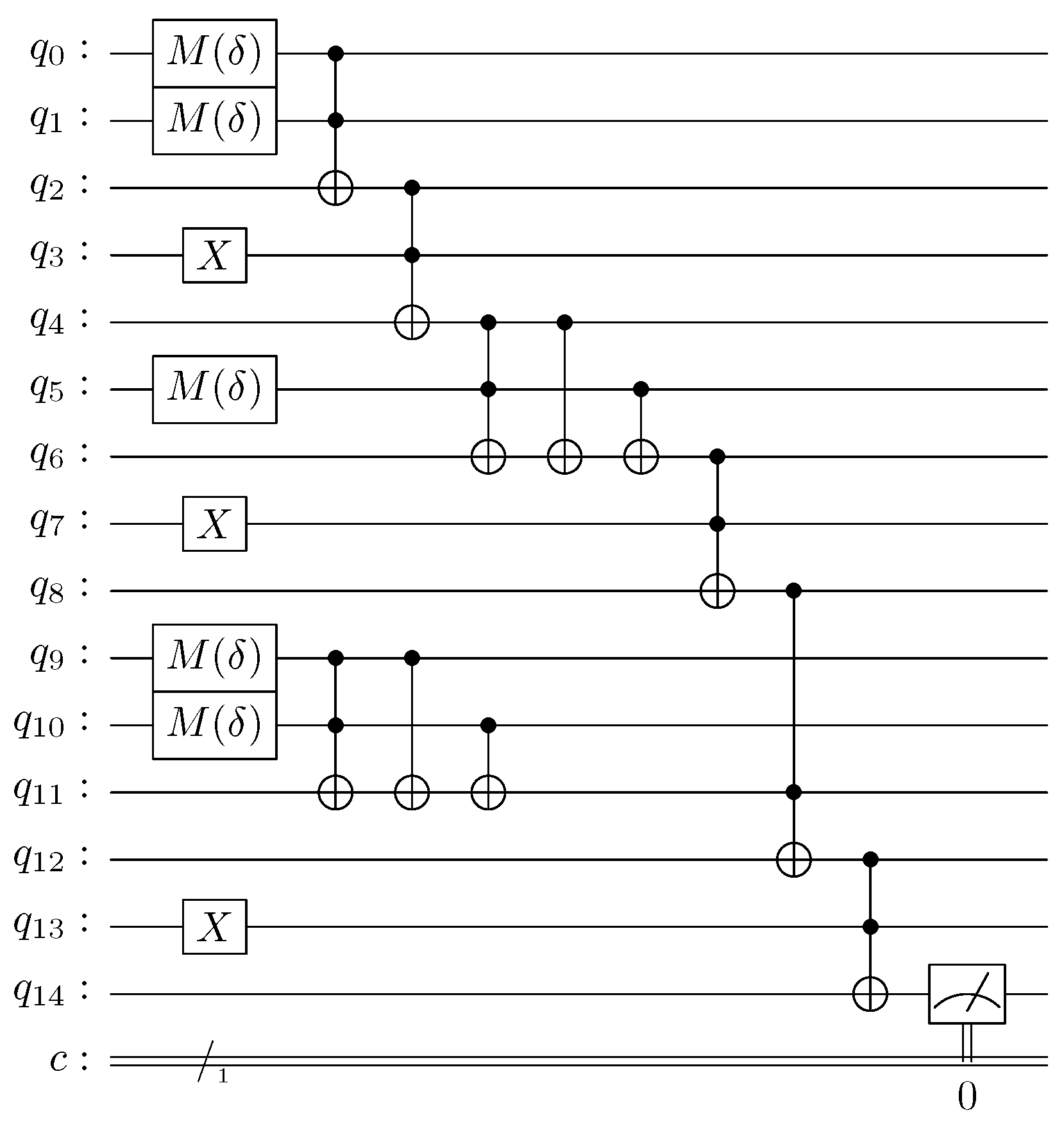
5.1. Experiment 1: Inaccuracy in Declarative Knowledge (Imprecision)
If we want to test our model for dealing with imprecision,
Figure 9 has to be modified as shown in
Figure 11.
The Hadamard gates of quantum lines , , , , and were replaced by gates, so as to configure inaccurate inputs. The Hadamard gates of quantum lines , , and were substituted by X gates, in order to set the causal relationships of the rules totally true (no uncertainty).
Table 7 illustrates the input data that allow us to compare the classical approach and the quantum approach for dealing with imprecision and the results obtained after running both the classical and quantum inferential circuits.
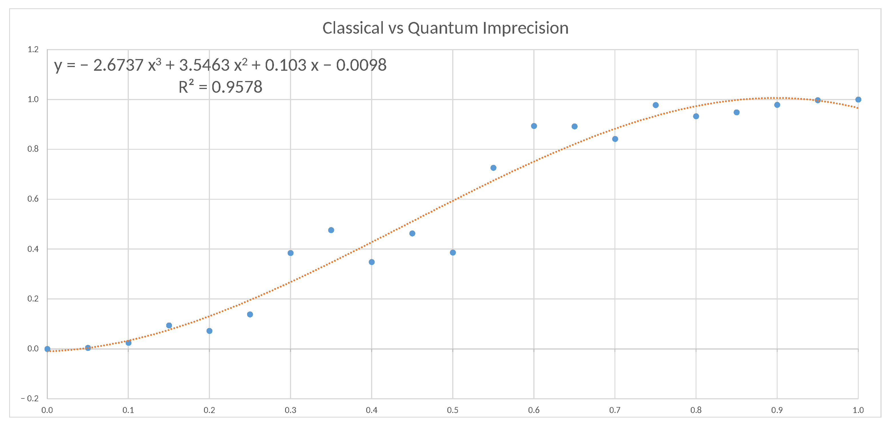
Figure 12 illustrates the results obtained for the imprecision experiment and shows a high level of correlation between classical and quantum approaches, which follows a polynomial distribution.
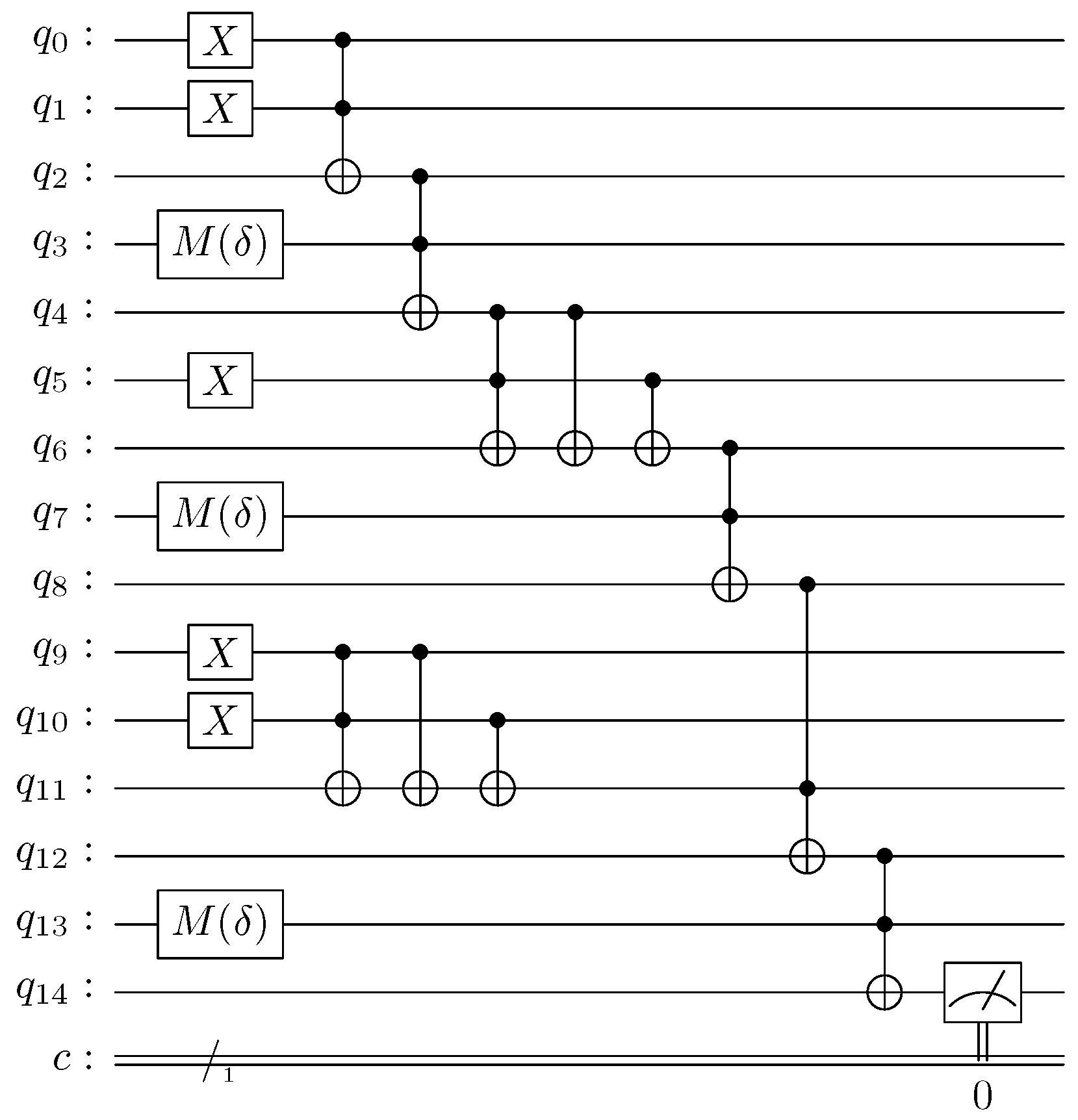
5.2. Experiment 2: Inaccuracy in Procedural Knowledge (Uncertainty)
If we want to test our model for dealing with uncertainty,
Figure 9 has to be modified as shown in
Figure 13.
The Hadamard gates of quantum lines , , and were replaced by gates, so as to configure inaccurate rules. The Hadamard gates of quantum lines , , , , and were substituted by X gates, in order to set the veracity of the facts totally true (no imprecision).
Table 8 illustrates the input data that allow us to compare the classical approach and the quantum approach for dealing with uncertainty and the results obtained after running both the classical and quantum inferential circuits.
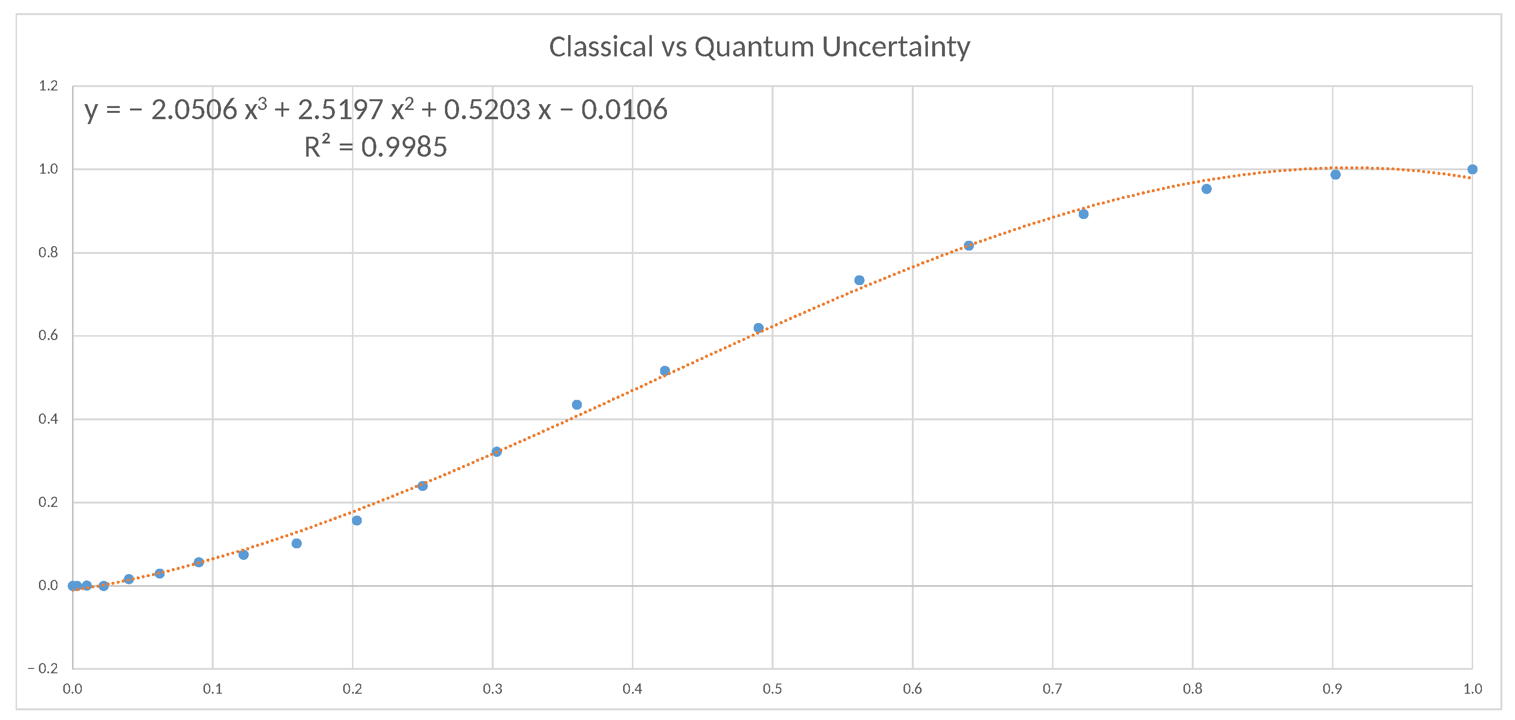
Figure 14 illustrates the results obtained for the uncertainty experiment and shows a high level of correlation between classical and quantum approaches, that follow a polynomial distribution.
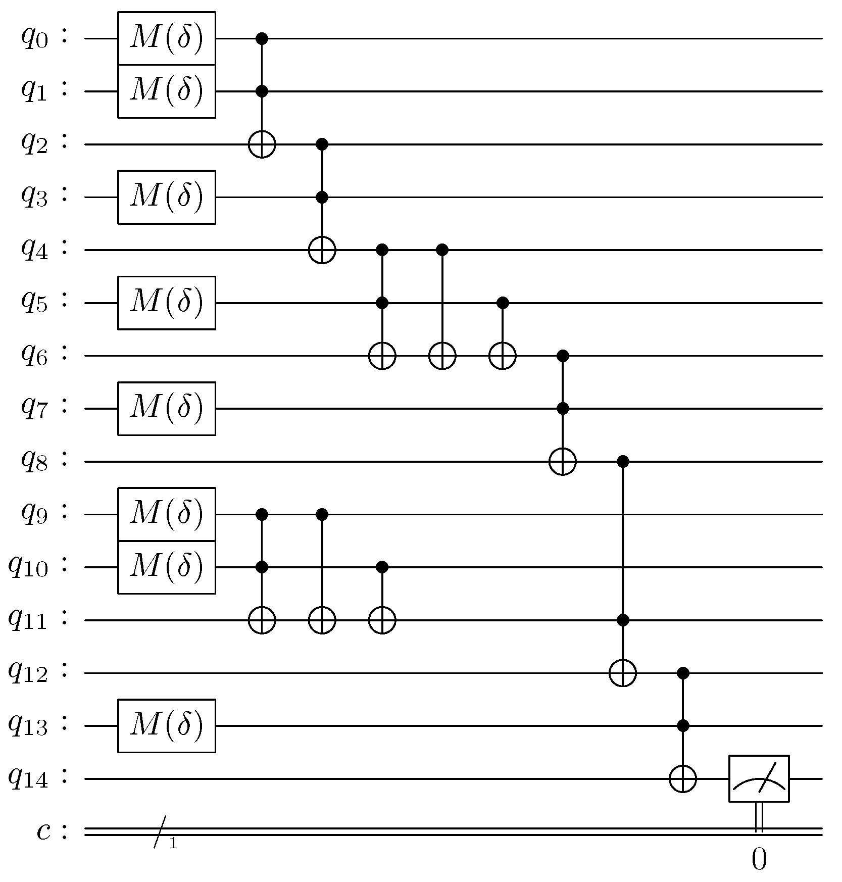
5.3. Experiment 3: Inaccuracy in Declarative and Procedural Knowledge (Imprecision and Uncertainty)
If we want to test our model for dealing with imprecision and uncertainty simultaneously,
Figure 9 has to be modified as shown in
Figure 15.
The Hadamard gates of quantum lines , , , , and were replaced by gates, so as to configure inaccurate inputs. The Hadamard gates of quantum lines , , and were substituted by gates so as to configure inaccurate rules.
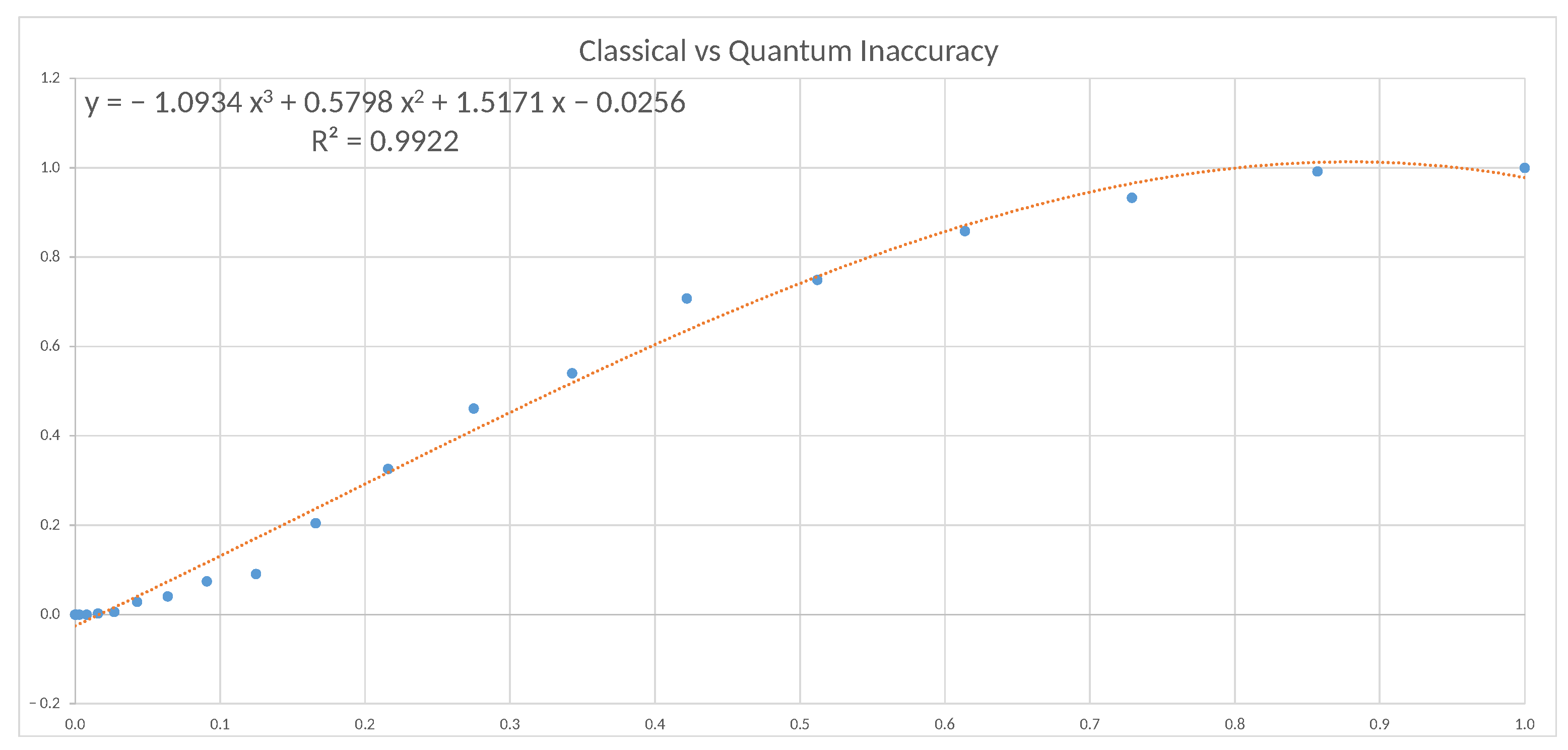
Table 9 illustrates the input data that allow us to compare the classical approach and the quantum approach for dealing with imprecision and uncertainty simultaneously and the results obtained after running both the classical and quantum inferential circuits.
Figure 16 illustrates the results obtained for the imprecision and uncertainty experiment and shows a high level of correlation between classical and quantum approaches, following a polynomial distribution.
6. Discussion
The main objective of this work was to check whether classical inaccurate knowledge can be implemented on a quantum architecture. For this, we chose a classical model for management of inexact knowledge, as the Certainty Factors Model of Shortliffe and Buchanan is. Said model, apparently without a clear theoretical basis, makes use of the principles of probability, both in the form of total probabilities and conditional probabilities, which in any case are subjective in nature.
Our work does not pretend to be an extension or revision of certainty factors per se but rather a new treatment of inaccurate reasoning through quantum computing. Certainty factors are used to compare our work to a previous classical model of inaccurate reasoning.
Given that we are in an age in which quantum computing is a fertile and current field of research and development, the fundamental question was to investigate whether the supposedly probabilistic behaviour of the certainty factors can be simulated by means of a quantum theory based on the quantum circuit model. In this sense, three different situations were considered: (1) inaccuracy in declarative knowledge, which we call imprecision, (2) inaccuracy in procedural knowledge that we call uncertainty, and (3) imprecision and uncertainty together.
For this, a use case consisting of an inferential circuit was designed that was implemented according to a classical philosophy and according to a quantum philosophy. The results obtained clearly show that there is a correlation between the results of the classical model and the results of the quantum model. In addition, not only is there a correlation, but this correlation is high, which results in striking. This may be a consequence of the ad hoc nature of the model of certainty factors, which is why we cannot confirm the strict probabilistic nature of this model. However, the great correlation between the results obtained for the classical and quantum approaches allows us to suspect that, indeed, the concept of probability underlies the concept of the certainty factor. We make this claim since quantum computing is inherently probabilistic.
Moreover, the plot of the results shows a clear similarity to the sigmoid function, which is widely used in other fields of Artificial Intelligence, such as Machine Learning, for example, in order to model the transmission of knowledge in support vector machines or neural networks [
36]. Thus, while it may be too early to assert the following statement, we think that this new quantum approach could be useful for the sake of knowledge transmission through inferential circuits, although we need to work further in the subject in order to make a clear statement about this hypothesis.
Analysing each of the scenarios, we verify that when we only use imprecision, the correlation coefficient between both models is 0.9578, which allows us to suspect that indeed classical imprecision and quantum imprecision can become extrapolated. If we analyse the second of the scenarios, in which we only consider uncertainty, we find a polynomial correlation coefficient of 0.9985, which represents a qualitative and quantitative leap that almost allows us to affirm that said correlation is more than a suspicion. Analysing the two scenarios separately, the largest deviations are obtained with imprecision rather than uncertainty. When we analyse the third scenario, that is, considering both imprecision and uncertainty, the polynomial correlation coefficient is 0.9922, which, being high, is located between the two previous extreme cases. This is undoubtedly due to the fact that imprecision penalises uncertainty; therefore, we can deduce that the hybrid model behaves as expected.
Regarding the future work, we consider that the approach we presented here could take advantages from quantum tools, such as instantaneous quantum polynomial (IQP) circuits [
37]. However, this work is reserved for following publications, since it would be out of the scope of this paper.
In addition, in the context of artificial intelligence and inaccurate knowledge, it could be interesting to develop a quantum implementation of other models of inexact knowledge treatment, such as fuzzy models [
17], the evidential theory of Dempster and Shafer [
18], or the Bayesian networks [
19]. Some work has already been conducted in this area, and the results seem promising. For example, Nabadan [
38] suggested the algebraic connections between classical logic and its generalizations, such as fuzzy logic and quantum logic, and Vourdas [
39] proposed an interpretation of quantum probabilities as Dempster–Shafer probabilities and Borujeni et al. developed a quantum circuit representation of Bayesian networks [
40].


