A Novel RBF Collocation Method Using Fictitious Centre Nodes for Elasticity Problems

Abstract

The traditional radial basis function collocation method (RBFCM) has poor stability when solving two-dimensional elastic problems, and the numerical results are very sensitive to shape parameters, especially in solving elastic problems. In this paper, a novel radial basis function collocation method (RBFCM) using fictitious centre nodes is applied to the elastic problem. The proposed RBFCM employs fictitious centre nodes to interpolate the unknown coefficients, and is much less sensitive to the shape parameter compared with the traditional RBFCM. The details of the shape parameters are discussed for the novel RBFCM in elastic problems. Elastic problems with and without analytical solutions are given to show the effectiveness of the improved RBFCM.

1. Introduction

Over the past few decades, one type of the popular numerical methods that have been used for solving scientific and engineering problems has been the mesh-based methods, such as the finite element method (FEM) [1,2], finite difference method [3], finite volume method [4], and so on [5]. However, mesh-based methods face huge challenges and difficulties when dealing with large deformations. In recent years, meshless methods have been developed for their simplicity and effectiveness. Without grid division, the meshless methods have obvious advantages in solving complex domains, moving boundaries, and high-dimensional problems.

The Kansa method or RBFCM is one type of meshless method based on the collocation technique [6]. The uniqueness and convergence of the RBFCM have been investigated [7,8]. However, in the RBFCM simulation process, an asymmetric and fully populated matrix of a system of the linear equations is generated, which may cause a high condition number and affect the stability of the method. In order to deal with the asymmetric matrix, some methods have been proposed and developed to avoid the difficulties associated with the asymmetric matrix, such as the RBF Hermite collocation method [9] and the modified Kansa’s method (MKM) [10]. In the traditional RBFCM, the centre and collocation nodes are the same. The matrix formulated in the RBFCM is ill-conditioned, and the traditional RBFCM is not stable, especially in dealing with Neumann boundary conditions [11]. The boundary conditions should be treated properly by using the weighted RBFCM and other numerical techniques [12,13].

The shape parameter of the traditional RBFCM should really be taken care of, and the accuracy of the traditional RBFCM is related to the shape parameters. Many numerical algorithms have been put forward to pick out the optimal shape parameters, such as the leave-one-out cross-validation (LOOCV) algorithm [14], the genetic algorithm [15], and the golden section search algorithm [16]. Thus, the RBFCM is not easy to apply to elastic problems, especially when the solution is not smooth [17,18].

Recently, a novel RBFCM using fictitious centre nodes has been proposed with high stability and accuracy [19]. Unlike the traditional RBFCM, the idea employs fictitious nodes as the centre nodes, and the fictitious nodes are distributed in a larger area covering the original domain. This process greatly improves the performance of the RBFCM. To some extent, this idea is similar to using an imaginary source node outside the domain in the method of fundamental solutions [20]. However, the proposed method has not been applied to the elastic problems since the field quantity of the elastic problems is generally not smooth. In this work, the improved RBFCM has firstly been employed on the elastic problems with the multi-quartic (MQ) RBF. Here, the modified Franke formula [21] and the sample solution approach [22,23] are considered in the proposed RBFCM for the elastic problems [24,25,26,27]. This paper is organized as follows:

In Section 2, the basic equations of the elastic problem are introduced. In Section 3, the numerical formulation of the traditional RBFCM and the improved method with fictitious centres are elaborated on with details. Section 4 presents several approaches to choosing shape parameters. In Section 5, four different numerical examples are given to demonstrate the effectiveness of the proposed method. Finally, some remarks and future research works are provided in the last section.

2. Elastic Problem

2.1. Two-Dimensional Cases

The governing equations of the plane stress elasticity problem [28] can be expressed as

$$\frac{E}{1-{\mu }^2}(\frac{{\partial }^2{u}_1}{\partial x_{}^2}+\frac{1-\mu }{2}\frac{{\partial }^2{u}_1}{\partial y_{}^2}+\frac{1+\mu }{2}\frac{{\partial }^2{u}_2}{\partial x_{}\partial y})+f_1(x,y)=0,\hspace{1em}(x,y)\in \mathsf{\Omega },$$

(1)

$$\frac{E}{1-{\mu }^2}(\frac{{\partial }^2{u}_2}{\partial y_{}^2}+\frac{1-\mu }{2}\frac{{\partial }^2{u}_2}{\partial x_{}^2}+\frac{1+\mu }{2}\frac{{\partial }^2{u}_1}{\partial x_{}\partial y})+f_2(x,y)=0,\hspace{1em}(x,y)\in \mathsf{\Omega },$$

(2)

where μ is Poisson’s ratio and E is the elasticity modulus, $u_i\left(x,y\right), i=1, 2$ are the displacements, and $f_i(x,y), i=1, 2$ are the forcing terms. $\mathsf{\Omega }$ is a domain bounded by a segmented smooth surface. The traction boundary conditions can be expressed as follows

$$\frac{E}{1-{\mu }^2}[n_1(\frac{\partial u_1}{\partial x}+\mu \frac{\partial u_2}{\partial y}{)}_s+n_2\frac{1-\mu }{2}(\frac{\partial u_1}{\partial y}+\frac{\partial u_2}{\partial x}{)}_s]={\overline{f}}_1(x,y),\hspace{1em}(x,y)\in \partial {\mathsf{\Omega }}^N,$$

(3)

$$\frac{E}{1-{\mu }^2}[n_2(\frac{\partial u_2}{\partial y}+\mu \frac{\partial u_1}{\partial x}{)}_s+n_1\frac{1-\mu }{2}(\frac{\partial u_2}{\partial x}+\frac{\partial u_1}{\partial y}{)}_s]={\overline{f}}_2(x,y),\hspace{1em}(x,y)\in \partial {\mathsf{\Omega }}^N,$$

(4)

where $n_i(x,y), i=1, 2$ are the unit normal vectors at the boundary node. $\partial {\mathsf{\Omega }}^N$ is the boundary that satisfies traction boundary conditions, ${\overline{f}}_i(x,y),i=1,2$ are the tractions. The displacement boundary conditions can be given as

$$u_1(x,y)=g_1(x,y),\hspace{1em}(x,y)\in \partial {\mathsf{\Omega }}^D,$$

(5)

$$u_2(x,y)=g_2(x,y),\hspace{1em}(x,y)\in \partial {\mathsf{\Omega }}^D,$$

(6)

$g_i(x,y),i=1,2$ represent the displacement at boundary nodes. $\partial {\mathsf{\Omega }}^D$ is the boundary that satisfies Dirichlet boundary conditions. For the plane strain problem, the governing equation and boundary conditions can be obtained only by changing $E$ to $E/\left(1-{\mu }^2\right)$ and $\mu$ to $\mu /\left(1-\mu \right)$ in the Equations (1)–(6).

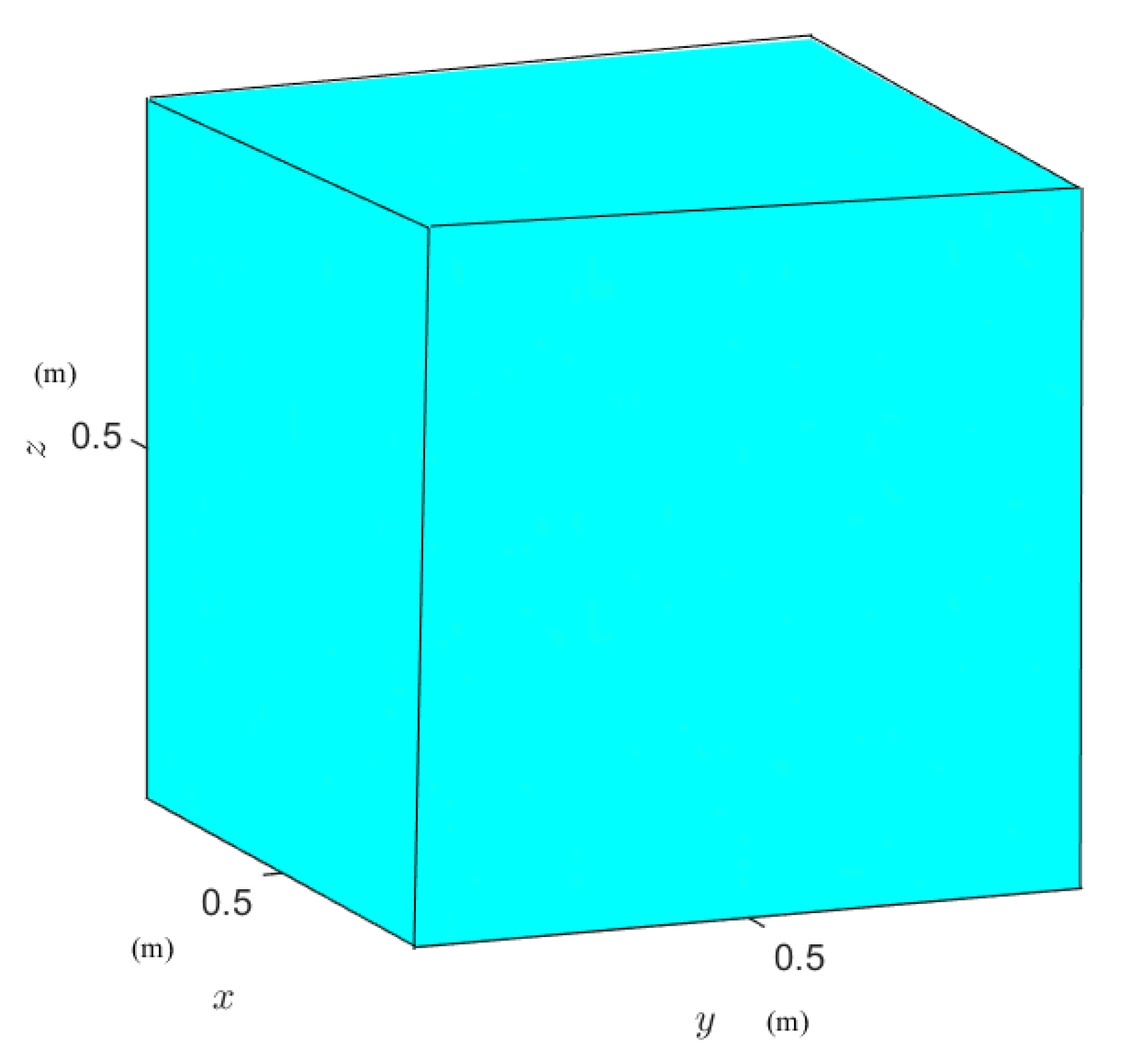
2.2. Three-Dimensional Cases

The governing equations of the three-dimensional elasticity problem [28] can be expressed as

$$\left.\begin{array}{l}{\sigma }_{11}=\frac{E}{1+\mu }(\frac{\mu }{1-2\mu }\theta +\frac{\partial u_1}{\partial x}),\\ {\sigma }_{22}=\frac{E}{1+\mu }(\frac{\mu }{1-2\mu }\theta +\frac{\partial u_2}{\partial y}),\\ {\sigma }_{33}=\frac{E}{1+\mu }(\frac{\mu }{1-2\mu }\theta +\frac{\partial u_3}{\partial z}),\\ {\sigma }_{23}=\frac{E}{2(1+\mu )}(\frac{\partial u_3}{\partial y}+\frac{\partial u_2}{\partial z}),\\ {\sigma }_{31}=\frac{E}{2(1+\mu )}(\frac{\partial u_1}{\partial z}+\frac{\partial u_3}{\partial x}),\\ {\sigma }_{12}=\frac{E}{2(1+\mu )}(\frac{\partial u_1}{\partial y}+\frac{\partial u_2}{\partial x}),\end{array}\right\}$$

(7)

where $\theta =\frac{\partial u_1}{\partial x}+\frac{\partial u_2}{\partial y}+\frac{\partial u_3}{\partial z}.$ μ is Poisson’s ratio and E is the elasticity modulus. $u_i, i=1, 2, 3$ are the displacements. ${\sigma }_{ij}, i, j=1, 2, 3$ are the stresses. The governing equations of the 3D elasticity problem can be expressed as

$$\begin{array}{l}\frac{\partial {\sigma }_{11}}{\partial x}+\frac{\partial {\sigma }_{21}}{\partial y}+\frac{\partial {\sigma }_{31}}{\partial z}+f_1=0,\hspace{1em}(x,y,z)\in \mathsf{\Omega },\\ \frac{\partial {\sigma }_{22}}{\partial y}+\frac{\partial {\sigma }_{32}}{\partial z}+\frac{\partial {\sigma }_{12}}{\partial x}+f_2=0,\hspace{1em}(x,y,z)\in \mathsf{\Omega },\\ \frac{\partial {\sigma }_{33}}{\partial z}+\frac{\partial {\sigma }_{13}}{\partial x}+\frac{\partial {\sigma }_{23}}{\partial y}+f_3=0,\hspace{1em}(x,y,z)\in \mathsf{\Omega },\end{array}$$

(8)

where $f_i, i=1, 2, 3$ are the forcing terms, $\mathsf{\Omega }$ is a 3D computational domain. The traction boundary conditions can be expressed as follows

$$\begin{array}{l}{n}_1{\left({\sigma }_{11}\right)}_s+n_2\left({\sigma }_{21}\right){}_s+n_3{\left({\sigma }_{31}\right)}_s={\overline{f}}_1,\hspace{1em}(x,y,z)\in \partial {\mathsf{\Omega }}^N\\ n_2{\left({\sigma }_{22}\right)}_s+n_3\left({\sigma }_{32}\right){}_s+n_1{\left({\sigma }_{12}\right)}_s={\overline{f}}_2,\hspace{1em}(x,y,z)\in \partial {\mathsf{\Omega }}^N\\ n_3{\left({\sigma }_{33}\right)}_s+n_1\left({\sigma }_{13}\right){}_s+n_2{\left({\sigma }_{23}\right)}_s={\overline{f}}_3,\hspace{1em}(x,y,z)\in \partial {\mathsf{\Omega }}^N\end{array}$$

(9)

where $n_i, i=1, 2, 3$ are the unit normal vectors at the boundary node. $\partial {\mathsf{\Omega }}^N$ is the boundary that satisfies traction boundary conditions, ${\overline{f}}_i(x,y),i=1, 2, 3$ are the tractions. The displacement boundary conditions can be given as

$$\begin{array}{l}{u}_1=g_1,\hspace{1em}(x,y,z)\in \partial {\mathsf{\Omega }}^D, \\ u_2=g_2,\hspace{1em}(x,y,z)\in \partial {\mathsf{\Omega }}^D,\\ u_3=g_3,\hspace{1em}(x,y,z)\in \partial {\mathsf{\Omega }}^D,\end{array}$$

(10)

$g_i,i=1, 2, 3$ represent the displacement at boundary nodes. $\partial {\mathsf{\Omega }}^D$ is the boundary that satisfies Dirichlet boundary conditions.

3. Numerical Methods and Discretization

3.1. The RBFCM

Here we take the 2D elastic problem as an example. In the RBFCM [6], the displacements of the 2D elastic problem can be approximated as

$$u_1^n\left(x,y\right)={\displaystyle \sum _{j=1}^N{\overline{\xi }}_{1,j}{\varphi }_j}(x,y),$$

(11)

$$u_2^n\left(x,y\right)={\displaystyle \sum _{j=1}^N{\overline{\xi }}_{2,j}{\varphi }_j}(x,y),$$

(12)

where $N$ is the number of centre nodes, ${\overline{\xi }}_{1,j}$ and ${\overline{\xi }}_{2,j}$ are the unknown coefficients related to the numerical solutions $u_1^n$ and $u_2^n$, respectively; ${\varphi }_j$ is the RBF, in this work the multi-quadric (MQ) RBF is given as follows

$${\varphi }_j\left(x,y\right)=\sqrt{{\left(x-{\overline{x}}_j\right)}^2+{\left(y-{\overline{y}}_j\right)}^2+c^2},$$

(13)

The RBF is associated with centre nodes $({\overline{x}}_j,{\overline{y}}_j)$, which are the same as the collocation nodes $(x_k,y_k)$ in the traditional RBFCM, as shown in Figure 1. $c$ is the shape parameter. $K_i$ is the number of collocation nodes ${\left.\left\{(x_k,y_k)\right.\right\}}_{k=1}^{K_i}$ in $\mathsf{\Omega }$, $K_{b1}$ is the number of boundary nodes ${\left.\left\{x_k,y_k\right.\right\}}_{k=K_i+1}^{K_i+K_{b1}}$ on $\partial {\mathsf{\Omega }}^N$, $K_{b2}$ is the number of boundary nodes ${\left.\left\{x_k,y_k\right.\right\}}_{k=K_i+K_{b1}+1}^{K_i+K_{b1}+K_{b2}}$ on $\partial {\mathsf{\Omega }}^D$, and $K=K_i+K_{b1}+K_{b2}$ is the number of total nodes. In the traditional RBFCM $K=N$.

By substituting Equations (7) and (8) back to the governing equations in Equations (1) and (2), the following discretized form can be obtained

$$\frac{E}{1-{\mu }^2}\left({\displaystyle \sum _{j=1}^N{\overline{\xi }}_{1,j}}{h}_{j,k}^{(1)}+{\displaystyle \sum _{j=1}^N{\overline{\xi }}_{2,j}}{h}_{j,k}^{(2)}\right)+f_1=0,$$

(14)

$$\frac{E}{1-{\mu }^2}\left({\displaystyle \sum _{j=1}^N{\overline{\xi }}_{1,j}}{h}_{j,k}^{(2)}+{\displaystyle \sum _{j=1}^N{\overline{\xi }}_{2,j}}{h}_{j,k}^{(3)}\right)+f_2=0,$$

(15)

where

$$\left\{\begin{array}{l}{h}_{j,k}^{(1)}=\frac{{\partial }^2{\varphi }_j(x_k,y_k)}{\partial x^2}+\frac{1-\mu }{2}\frac{{\partial }^2{\varphi }_j(x_k,y_k)}{\partial y^2},\\ h_{j,k}^{(2)}=\frac{1+\mu }{2}\frac{{\partial }^2{\varphi }_j(x_k,y_k)}{\partial x\partial y},\\ h_{j,k}^{(3)}=\frac{{\partial }^2{\varphi }_j(x_k,y_k)}{\partial y^2}+\frac{1-\mu }{2}\frac{{\partial }^2{\varphi }_j(x_k,y_k)}{\partial x^2},\end{array}\right.$$

(16)

where $k=1,\dots ,K_i$, is the index of the number of the inner nodes. Equations (13) and (14) can be obtained by substituting Equations (7) and (8) back to traction boundary conditions in Equations (3) and (4).

$$\frac{E}{1-{\mu }^2}\left[{\displaystyle \sum _{j=1}^N{\overline{\xi }}_{1,j}}{s}_{j,k}^{(1)}+{\displaystyle \sum _{j=1}^N{\overline{\xi }}_{2,j}}{s}_{j,k}^{(2)}\right]={\overline{f}}_1,$$

(17)

$$\frac{E}{1-{\mu }^2}\left[{\displaystyle \sum _{j=1}^N{\overline{\xi }}_{1,j}}{s}_{j,k}^{(3)}+{\displaystyle \sum _{j=1}^N{\overline{\xi }}_{2,j}}{s}_{j,k}^{(4)}\right]={\overline{f}}_2,$$

(18)

where

$$\left\{\begin{array}{l}{s}_{j,k}^{(1)}=n_1\frac{\partial {\varphi }_j(x_k,y_k)}{\partial x}+n_2\frac{1-\mu }{2}\frac{\partial {\varphi }_j(x_k,y_k)}{\partial y},\\ s_{j,k}^{(2)}=n_1\mu \frac{\partial {\varphi }_j(x_k,y_k)}{\partial y}+n_2\frac{1-\mu }{2}\frac{\partial {\varphi }_j(x_k,y_k)}{\partial x},\\ s_{j,k}^{(3)}=n_2\mu \frac{\partial {\varphi }_j(x_k,y_k)}{\partial x}+n_1\frac{1-\mu }{2}\frac{\partial {\varphi }_j(x_k,y_k)}{\partial y},\\ s_{j,k}^{(4)}=n_2\frac{\partial {\varphi }_j(x_k,y_k)}{\partial y}+n_1\frac{1-\mu }{2}\frac{\partial {\varphi }_j(x_k,y_k)}{\partial x},\end{array}\right.$$

(19)

$k=K_i+1,\dots ,K_i+K_{b1}$ is the index of the number of the boundary nodes that satisfy the traction boundary conditions. Equations (16) and (17) can be obtained by substituting Equations (7) and (8) back to the displacement boundary conditions in Equations (5) and (6).

$${\displaystyle \sum _{j=1}^N{\overline{\xi }}_{1,j}{\varphi }_j(x_k,y_k)}=g_1,$$

(20)

$${\displaystyle \sum _{j=1}^N{\overline{\xi }}_{2,j}{\varphi }_j(x_k,y_k)}=g_2,$$

(21)

$k=K_i+K_{b1}+1,\dots ,K_i+K_{b1}+K_{b2}$ is the index of the number of the boundary nodes that satisfy the Dirichlet boundary conditions. Generally, we choose K ≥ N. The unknown coefficients ${\left\{\left.{\overline{\xi }}_{1,n}\right\}\right.}_{n=1}^N$ and ${\left\{\left.{\overline{\xi }}_{2,n}\right\}\right.}_{n=1}^N$ can be calculated from the linear system obtained from Equations (10)–(17). Then, the displacements of Equations (1)–(6) can be approximated by Equations (7) and (8). The collocation and the centre nodes are the same in the RBFCM, and the size of the system matrix is $2K\times 2N$, where K = N here.

3.2. The Improved RBFCM with Fictitious Centre Nodes

In the improved RBFCM, the collocation nodes and centre nodes are different. A set of ghost nodes are taken as fictitious centres, as the red nodes shown in Figure 2. The number of the fictitious nodes is defined as K. The fictitious centre nodes can be placed inside and outside the domain, as shown in Figure 2. The size of the fictitious centre nodes can be controlled by a radius of R. The relationship of the distance in the RBFCM is changed with such a simple adjustment. To study the performance of the improved RBFCM, the shape parameters and the values of radius R require further study.

4. Shape Parameters

Over the past two decades, various algorithms have been proposed to predict the optimal shape parameter in the RBFCM. The shape parameter is vital for the performance of the RBFCM in different problems. In this work, three different approaches are considered for choosing shape parameters in the improved RBFCM for the elastic problem.

Approach 1: Brute force (BF)

A typical method to find an optimal c is the “brute force” method, in which the value of the shape parameter starts from c = 0.01, increasing by 0.01 each time until c arrives at a certain value. Then an optimal shape parameter can be decided by using the trial errors obtained from different shape parameters. The BF costs a lot of time in the repeating process, and it is not an efficient way to find the optimal shape parameter. The time costs of the “brute force” method can be dramatically reduced by using the modified Franke formula.

Approach 2: The modified Franke formula (MFF)

In 1982, an experimental formula based on the density of the interpolation nodes was proposed by Franke to estimate the optimal shape parameter [21]. Recently, owing to the popularity of double precision arithmetic, the Franke formula has been revised to $c=D/\left(0.8\sqrt[4]{N}\right)$, where D is the diameter of the smallest circle containing all fictitious centre nodes and N is the number of the collocation nodes. The modified Franke formula has been demonstrated to be a satisfactory prediction for a reasonably good shape parameter of the multi-quadric (MQ) radial basis function.

Approach 3: The sample solution approach (SSA)

When the analytical solutions are unavailable, the sample solution approach (SSA) is employed to validate the numerical results [23]. In the procedure of the SSA, an exact solution to the pseudo-problem is set up as the sample solution. The pseudo-problem has the same geometry and the same number of degrees of freedom as the current problem. The optimal shape parameters of the pseudo-problem can be found with the help of the exact solutions. Then the optimal shape parameters obtained from the pseudo-problem are used to solve the problem where the exact solution is not available.

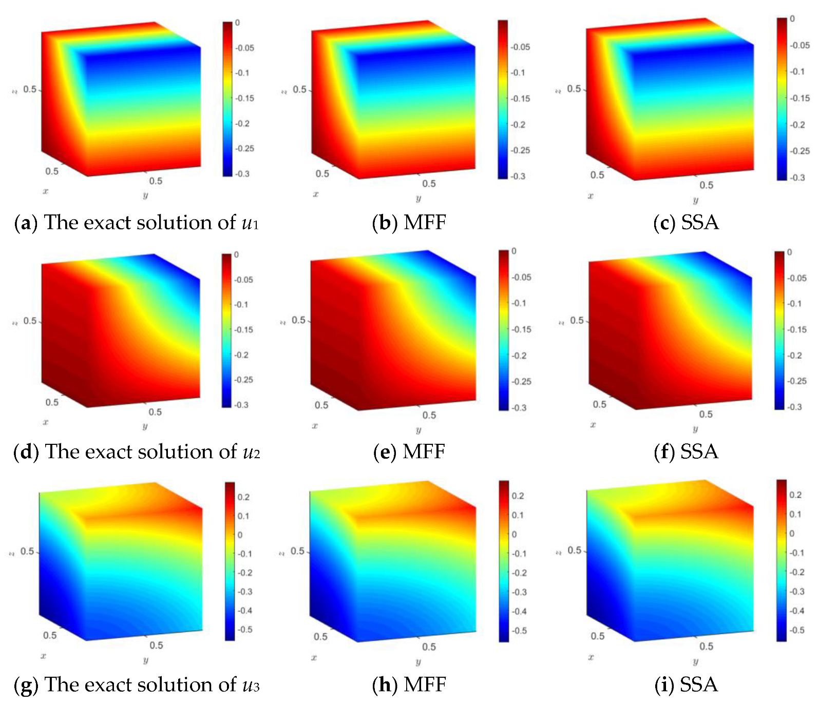
5. Numerical Results

In this section, an example with an exact solution is presented to illustrate the effectiveness of an improved RBFCM, and then two other numerical examples of two-dimensional elastic problems without exact solutions are presented by comparing them with the numerical results of the finite element method. The fictitious centre nodes are distributed by using the Halton quasi-random number generator, which is available via the MATLAB command haltonset. The relative error is defined as follows

$$RE=\sqrt{{\displaystyle \sum _{}^{}{({\mathit{u}}_{}^n-\mathit{u})}^2}}/\sqrt{{\displaystyle \sum _{}^{}{(\mathit{u})}^2}},$$

(22)

where ${\mathit{u}}_{}^n$ and $\mathit{u}$ are the numerical and analytical solutions of the displacement, respectively.

Example 1.

In this example, the plan strain problem described in Equations (1)–(6) is considered, where$E$is replaced with$E/\left(1-{\mu }^2\right)$and$\mu$is replaced with$\mu /\left(1-\mu \right)$. The modulus of elasticity is taken to be E = 2.1 × 10⁵ Mpa, and$\mu =0.2$. The computational domain with node distributions is shown in Figure 3, where a 2 m × 2 m square elastic plate with 100 circular holes (radius = 0.05 m) is presented. The traction boundary conditions are applied to the four boundaries of the square domain, and the displacement boundary conditions are imposed on the inner boundaries of 100 circular holes. The analytical solutions are given as

$$u_1=xy/\left[2(1+\mu )G\right],u_2=-\left(y^2-x^2\right)/\left[4(1+\mu )G\right]$$

The node distribution of the improved RBFCM is shown in Figure 4, where 1296 fictitious centre nodes (red circle “○”) are given to evaluate the numerical results. Unlike the traditional RBFCM, the fictitious centre nodes are placed in a larger circular area with R = 3. The numerical results of the improved RBFCM are compared with the results obtained with the traditional RBFCM in Figure 5.

In Figure 5, the relative errors of the displacements computed by the traditional and the improved RBFCM are shown with the red and blue colors, respectively. Different shape parameters are used to evaluate the relative errors of both traditional and improved RBFCM. The numerical results show that the numerical results of the improved RBFCM are always much better than the traditional RBFCM. Moreover, when the shape parameter changes, the relative errors of the improved RBFCM are much smaller than 10⁻⁵, which indicates that the improved RBFCM is not sensitive to the variations in the shape parameters.

In Figure 5, the three different approaches to choosing shape parameters are tested for the improved RBFCM. The c_BF, c_SSA, and c_MFF are the optimal shape parameters calculated by the BF, SSA, and MFF, respectively. The relative errors of c_BF, c_SSA, and c_MFF in Figure 5 are less than 10⁻⁹. The BF, SSA, and MFF can also be applied to obtain the optimal shape parameter in the improved RBFCM.

Figure 6 displays the convergence rate of both the improved and traditional RBFCMs by considering the c_BF, c_SSA, and c_MFF. The relative errors of the displacements converge rapidly as the number of collocation nodes increases for both the improved and traditional RBFCMs. However, the relative errors of the improved RBFCM are much better than the traditional RBFCM. Again, the improved RBFCM is not sensitive to the shape parameters compared with the results of the traditional RBFCM.

As the improved RBFCM is influenced by the fictitious centre nodes, the influence of R is studied in

Table 1. The relative errors of the improved RBFCM with different R.

R	cMFF	RE	cSSA	RE	cBF	RE
2	1.291	1.30(−09)	1.146	7.94(−10)	0.929	2.62(−10)
3	1.936	1.70(−10)	1.047	4.81(−11)	1.224	6.71(−12)
4	2.582	1.64(−09)	1.146	5.08(−11)	1.698	1.14(−11)
5	3.227	2.30(−09)	1.854	1.07(−11)	1.757	8.08(−12)
6	3.873	2.18(−09)	2.047	2.82(−11)	2.053	4.19(−12)
7	4.518	6.83(−10)	2.236	1.02(−11)	2.112	1.12(−11)
8	5.164	3.47(−10)	1.815	4.33(−11)	2.527	5.44(−12)

.

In Table 1, 700 interior nodes and 600 boundary nodes are considered, thus 1300 ghost nodes are used to guarantee the size of the discretized matrix to be square. R changes from 2 to 8, and c_BF, c_SSA, and c_MFF are used to evaluate the optimal relative errors. The relative errors in Table 1 show that, as the value of R is larger than 2, the improved RBFCM can always obtain accurate results, which further indicate the stability of the improved RBFCM. Compared with the relative errors of c_BF, c_SSA, and c_MFF, the relative errors of c_BF are the best results; however, the relative errors of c_BF and c_SSA are also less than 10⁻⁹. The improved RBFCM is not sensitive to the shape parameter when R changes in a certain range.

Example 2.

As shown in Figure 7, a problem with the partition wall is considered. The density of the partition wall is ρ = 7800 kg/m³, the height is H = 1 m, and the thickness L = 0.5 m. The density of water is ρ₁ = 1000 kg/m³. The plane strain problem described in Equations (1)–(6) is considered, where E and μ are replaced with E/(1 − μ²) and μ/(1 − μ), respectively. Then E = 2.1 × 10⁵ Mpa, and μ = 0.3. In the numerical calculation, 361 interior nodes and 80 boundary nodes are considered, thus, 441 fictitious centre nodes are used to guarantee the discretized matrix is square.

The numerical error is defined as

$$RE=\sqrt{{\displaystyle \sum _{}^{}{({\mathit{u}}_{}^n-{\mathit{u}}_{}^f)}^2}}/\sqrt{{\displaystyle \sum _{}^{}{({\mathit{u}}_{}^f)}^2}},$$

(23)

where${\mathit{u}}_{}^n=\left[u_{1,1}^n,\dots ,u_{1,N_t}^n,u_{2,1}^n,\dots ,u_{2,N_t}^n\right]$and${\mathit{u}}_{}^f=\left[u_{1,1}^f,\dots ,u_{1,N_t}^f,u_{2,1}^f,\dots ,u_{2,N_t}^f\right]$are the numerical solutions obtained by the improved RBFCM and the FEM, respectively. N_t is the total number of test nodes.

Firstly, the displacements obtained from the improved RBFCM by considering different R are given in

Table 2. Relative errors by comparing with the FEM.

	MFF		SSA
R	c	RE	c	RE
4	2.182	0.024	1.799	0.019
5	2.728	0.025	0.880	0.022
6	3.273	0.027	1.178	0.017
7	3.819	0.027	1.072	0.039
8	4.364	0.028	1.139	0.045

. As the trial errors in the BF are not easy to decide without exact solutions, only the MFF and SSA are used to choose the optimal shape parameters. The numerical results are compared with the results of FEM, where 50,530 degrees of freedom (DOF) are used.

Results in Table 2 show that, as R changes from 4 to 8, the relative errors are always less than 5%. The shape parameter obtained from both SSA and MFF always leads to good numerical results for the improved RBFCM. To show the similarity of the results, the displacements on the x-axis and y-axis are given in Figure 8 and Figure 9, respectively. The numerical results are obtained from the improved RBFCM with R = 8.

Figure 8b and Figure 9b show the displacements obtained with the MFF. Figure 8c and Figure 9c show the results of SSA. Figure 8a and Figure 9a are the results of the FEM. Although the relative errors obtained by SSA are close to 5% in Table 2, the color maps of the displacements still show high similarity.

Example 3.

In this case, a rectangular cross-section of a vertical column with a fixed bottom is given in Figure 10. The density ρ = 7800 kg/m³, and a uniform shear q = 1 × 10⁷ N is imposed on the right side of the column. The length of the rectangular cross-section is L = 0.5 m and the height is H = 1 m. E = 2.1 × 10⁵ Mpa, and μ = 0.3. In the numerical calculations, 361 interior nodes and 80 boundary nodes are considered, and the number of ghost nodes is 441.

The results in

Table 3. Relative errors by comparing with the FEM.

	MFF		SSA
R	c	RE	c	RE
4	2.182	0.058	0.243	0.020
5	2.728	0.045	0.989	0.032
6	3.273	0.068	1.189	0.027
7	3.819	0.069	1.520	0.042
8	4.364	0.104	0.896	0.031

show that, as R changes from 4 to 7, the relative errors are always less than 8%. The relative errors obtained from MFF lead to worse numerical results for the improved RBFCM compared with SSA. When R = 8, the relative errors of MFF are close to 10%. The relative errors are larger compared with example 2; this is because the stress concentrations in this case are larger.

To show the similarity of the results, the displacements on the x-axis and y-axis are given in Figure 11 and Figure 12, respectively. The numerical results are obtained from the improved RBFCM with R = 8.

Figure 11b and Figure 12b show the displacements obtained with the MFF. Figure 11c and Figure 12c show the results of SSA. Figure 11a and Figure 12a are the results of the FEM. Although the relative error of the MFF in Table 3 is close to 10%, the color map of the displacements still shows a high similarity, which further validates the effectiveness of the improved RBFCM.

Example 4.

In this case, a 3D elastic problem is given as shown in Figure 13, with the length L = 1 m. Displacement boundary conditions are given to the lower bottom surface, and traction boundary conditions are given to the other surfaces. For more details of the problem please refer to [29]. The ghost nodes are evenly distributed inside the sphere, as shown in Figure 14.

The relative errors of the improved RBFCM are given and compared with the traditional RBFCM in Figure 15; the accuracy of the improved RBFCM is much higher than that of the traditional RBFCM, and as the number of nodes increases, the convergence rate of the improved RBFCM is much higher.

In

Table 4. The relative errors of the improved RBFCM with different R.

R	cMFF	RE	cSSA	RE
3	1.100	2.154(−05)	2.290	2.042(−06)
4	1.467	7.664(−06)	1.402	3.933(−06)
5	1.834	2.159(−05)	1.343	1.958(−06)
6	2.201	1.512(−05)	0.573	5.394(−06)
7	2.568	1.154(−05)	0.573	4.713(−06)
8	2.934	1.872(−05)	2.171	5.564(−06)
9	3.301	1.414(−05)	2.408	3.045(−06)
10	3.669	1.506(−05)	0.988	3.898(−06)

, the errors of different R using the optimal shape parameters obtained with the MFF and the SSA are given. In total, 729 interior nodes, 485 boundary nodes, and 1214 ghost nodes are considered, as shown in Figure 14. As shown in Table 4, with the MFF and the SSA used in the improved RBFCM, we can obtain an accurate solution.

The displacement contours are shown in Figure 16; the displacement contours of the improved RBFCM are similar to the exact solution. This further validates that the improved RBFCM can be extended to the 3D cases.

6. Conclusions

In this work, a novel RBFCM is proposed for elastic problems with high stability and accuracy. Elastic problems with and without analytical solutions are given to validate the improved RBFCM. Three different approaches to choosing shape parameters are tested in our examples. The numerical results show that the improved RBFCM has a high convergence rate and is less sensitive to the shape parameters. Moreover, the modified Franke formula and the sample solution approach adopted in this paper effectively settle the difficulty of choosing ideal shape parameters for the complex problems without analytical solutions, and further improve the accuracy, efficiency, and stability of the proposed method. One of our future research projects is to extend the proposed ghost node method to a local method for solving more practical real-life problems.

References

1. Bai, Y.; Wu, Y.; Xie, X. Uniform Convergence Analysis of a Higher Order Hybrid Stress Quadrilateral Finite Element Method for Linear Elasticity Problems. Adv. Appl. Math. Mech. 2016, 8, 399–425. [Google Scholar] [CrossRef]
2. Ge, Z.; Feng, M.; He, Y. Stabilized multiscale finite element method for the stationary Navier–Stokes equations. Math. Anal. Appl. 2009, 354, 708–717. [Google Scholar] [CrossRef] [Green Version]
3. Wu, H.-Y.; Duan, Y. Multi-quadric quasi-interpolation method coupled with FDM for the Degasperis–Procesi equation. Appl. Math. Comput. 2016, 274, 83–92. [Google Scholar] [CrossRef]
4. Li, J.; Liu, F.; Feng, L.; Turner, I. A novel finite volume method for the Riesz space distributed-order advection-diffusion equation. Appl. Math. Model. 2017, 46, 536–553. [Google Scholar] [CrossRef] [Green Version]
5. Steinberg, S.; Roache, P. Variational grid generation. Numer. Methods Part. Differ. Equ. 2010, 2, 71–96. [Google Scholar] [CrossRef]
6. Kansa, E. Multiquadrics—A scattered data approximation scheme with applications to computational flu-id-dynamics. II. Solutions to parabolic, hyperbolic and elliptic partial differential equations. Comput. Math. Appl. 1990, 19, 147–161. [Google Scholar] [CrossRef] [Green Version]
7. Madych, W.; Nelson, S. Multivariate interpolation and conditionally positive definite functions. Math. Comput. 1990, 54, 211–230. [Google Scholar] [CrossRef]
8. Micchelli, C. Interpolation of scattered data: Distance matrices and conditionally positive definite functions. Constr. Approx. 1986, 2, 11–22. [Google Scholar] [CrossRef]
9. Kansa, E.J.; Hon, Y.C. Circumventing the ill-conditioning problem with multiquadric radial basis functions: Applications to elliptic partial differential equations. Comput. Math. Appl. 2000, 39, 123–137. [Google Scholar] [CrossRef] [Green Version]
10. Nam, M.D.; Thanh, C.T. Mesh-free radial basis function network methods with domain decomposition for approximation of functions and numerical solution of Poisson’s equations. Eng. Anal. Bound. Elem. 2002, 26, 133–156. [Google Scholar]
11. Zheng, H.; Zhang, C.; Wang, Y.; Sladekc, J.; Sladek, V. Band structure computation of in-plane elastic waves in 2D phononic crystals by a meshfree local RBF collocation method. Eng. Anal. Bound. Elem. 2016, 66, 77–90. [Google Scholar] [CrossRef]
12. Hu, H.Y.; Chen, J.S.; Hu, W. Weighted radial basis collocation method for boundary value problems. Int. J. Numer. Methods Eng. 2006, 69, 2736–2757. [Google Scholar] [CrossRef]
13. Wang, L.; Qian, Z.; Zhou, Y.; Peng, Y. A weighted meshfree collocation method for incompressible flows using radial basis functions. J. Comput. Phys. 2019, 401, 108964. [Google Scholar] [CrossRef]
14. Fasshauer, G.; Zhang, J. On choosing optimal shape parameters for RBF approximation. Numer. Algorithms 2007, 45, 345–368. [Google Scholar] [CrossRef]
15. Esmaeilbeigi, M.; Hosseini, M. A new approach based on the genetic algorithm for finding a good shape parameter in solving partial differential equations by Kansa’s method. Appl. Math. Comput. 2014, 249, 419–428. [Google Scholar] [CrossRef]
16. Tsai, C.; Kolibal, J.; Li, M. The golden section search algorithm for finding a good shape parameter for meshless collocation methods. Eng. Anal. Bound. Elem. 2010, 34, 738–746. [Google Scholar] [CrossRef]
17. Xiong, J.; Wen, J.; Zheng, H. An improved local radial basis function collocation method based on the domain decomposition for composite wall. Eng. Anal. Bound. Elem. 2020, 120, 246–252. [Google Scholar] [CrossRef]
18. Zheng, H.; Yang, Z.; Zhang, C.; Tyrer, M. A local radial basis function collocation method for band structure computation of phononic crystals with scatterers of arbitrary geometry. Appl. Math. Model. 2018, 60, 447–459. [Google Scholar] [CrossRef]
19. Chen, C.; Karageorghis, A.; Dou, F. A novel RBF collocation method using fictitious centres. Appl. Math. Lett. 2019, 101, 106069. [Google Scholar] [CrossRef]
20. Golberg, M.; Chen, C. The method of fundamental solutions for potential, Helmholtz and diffusion problems. Bound. Integral Methods Numer. Math. Asp. 1998, 1, 103–176. [Google Scholar]
21. Franke, R. Scattered data interpolation: Tests of some methods. Math. Comput. 1982, 38, 181–200. [Google Scholar]
22. Kuo, L. On the Selection of a Good Shape Parameter for RBF Approximation and its Applications for Solving PDEs. Ph.D. Dissertation, University of Southern Mississippi, Hattiesburg, MS, USA, 2015. [Google Scholar]
23. Zheng, H. On the Selection of a Good Shape Parameter of the Localized Method of Approximated Particular Solutions. Adv. Appl. Math. Mech. 2018, 10, 896–911. [Google Scholar] [CrossRef]
24. Sarra, S.; Surgill, D. A random variable shape parameter strategy for radial basis function approaximation methods. Eng. Anal. Bound. Elem. 2009, 33, 1239–1245. [Google Scholar] [CrossRef]
25. Xiang, S.; Wang, K.-M.; Ai, Y.-T.; Sha, Y.-D.; Shi, H. Trigonometric variable shape parameter and exponent strategy for generalized multiquadric radial basis function approximation. Appl. Math. Model. 2011, 36, 1931–1938. [Google Scholar] [CrossRef]
26. Jankowska, M.A.; Karageorghis, A. Variable shape parameter Kansa RBF method for the solution of nonlinear boundary value problems. Eng. Anal. Bound. Elem. 2019, 103, 32–40. [Google Scholar] [CrossRef]
27. Kansa, E.; Carlson, R. Improved accuracy of multiquadric interpolation using variable shape parameters. Comput. Math. Appl. 1992, 24, 99–120. [Google Scholar] [CrossRef] [Green Version]
28. Timoshenko, S.P.; Goodier, J.N. Theory of Elasticity; McGraw-Hill: New York, NY, USA, 1934. [Google Scholar]
29. Meng, Z.; Fang, Y.; Cheng, Y. A Fast Element-Free Galerkin Method for 3D Elasticity Problems. Comput. Model. Eng. Sci. 2022, 132, 55–79. [Google Scholar] [CrossRef]
Figure 1. The node distribution of the traditional RBFCM (boundary nodes “●”, interior nodes “”).
Mathematics 10 03711 g001
Figure 2. The node distribution with fictitious centre nodes (boundary nodes “●”, interior nodes “” and fictitious centre nodes “”).
Mathematics 10 03711 g002
Figure 3. Computational domain with node distributions of the traditional RBFCM (boundary nodes “●”, interior nodes “”).
Mathematics 10 03711 g003
Figure 4. Node distributions of the improved RBFCM (boundary nodes “●”, interior nodes “” and fictitious centre nodes “”).
Mathematics 10 03711 g004
Figure 5. The numerical results versus the shape parameter.
Mathematics 10 03711 g005
Figure 6. Relative errors with a different number of collocation nodes when R = 6.
Mathematics 10 03711 g006
Figure 7. Problem of the partition wall.
Mathematics 10 03711 g007
Figure 8. Displacements of u1 calculated by the FEM and improved RBFCM.
Mathematics 10 03711 g008
Figure 9. Displacements of u2 calculated by the FEM and improved RBFCM.
Mathematics 10 03711 g009
Figure 10. Computational domain.
Mathematics 10 03711 g010
Figure 11. Displacements of u1 calculated by the FEM and improved RBFCM.
Mathematics 10 03711 g011
Figure 12. Displacements of u2 calculated by FEM and improved RBFCM.
Mathematics 10 03711 g012
Figure 13. Computational domain.
Mathematics 10 03711 g013
Figure 14. The nodes’ distributions.
Mathematics 10 03711 g014
Figure 15. Relative errors with different numbers of collocation nodes when R = 5.
Mathematics 10 03711 g015
Figure 16. Displacements of u1, u2, and u3 calculated by the improved RBFCM with R = 5.
Mathematics 10 03711 g016