The Sufficient Conditions for Orthogonal Matching Pursuit to Exactly Reconstruct Sparse Polynomials

Abstract

Orthogonal matching pursuit (OMP for short) is a classical method for sparse signal recovery in compressed sensing. In this paper, we consider the application of OMP to reconstruct sparse polynomials generated by uniformly bounded orthonormal systems, which is an extension of the work on OMP to reconstruct sparse trigonometric polynomials. Firstly, in both cases of sampled data with and without noise, sufficient conditions for OMP to recover the coefficient vector of a sparse polynomial are given, which are more loose than the existing results. Then, based on a more accurate estimation of the mutual coherence of a structured random matrix, the recovery guarantees and success probabilities for OMP to reconstruct sparse polynomials are obtained with the help of those sufficient conditions. In addition, the error estimation for the recovered coefficient vector is gained when the sampled data contain noise. Finally, the validity and correctness of the theoretical conclusions are verified by numerical experiments.

1. Introduction

It is well known that smooth functions have approximately sparse expansions under certain orthogonal systems. Therefore, one of the fundamental research problems in function approximation is the theoretical and algorithmic study of the exact reconstruction of the sparse polynomials [1,2,3,4,5,6]. In this paper, the form of the polynomial $g\left(x\right)$ is considered as

$$g\left(x\right)=\sum _{j\in \Lambda }{c}_j{\varphi }_j\left(x\right),$$

where ${\left\{{\varphi }_j\left(x\right)\right\}}_{j\in \Lambda }$ is a set of uniformly bounded orthonormal basis functions defined on $\Omega \subset {\mathbb{R}}^d$, $\Lambda$ is the index set with $|\Lambda |=n$, where $|\Lambda |$ denotes the number of elements in the set $\Lambda$, n can be finite or infinite. If the coefficient vector $\mathbf{c}={[c_1,\dots ,c_n]}^{\top }\in {\mathbb{R}}^{n\times 1}$ has at most s elements that are not zero, where $2\le s\ll n$, we call the polynomial $g\left(x\right)$ an s-sparse polynomial, and s is the sparsity of the polynomial $g\left(x\right)$ and the coefficient vector $\mathbf{c}$. Obviously, if the sparse coefficient vector $\mathbf{c}$ can be recovered exactly, the sparse polynomial $g\left(x\right)$ can be reconstructed. Therefore, we transform the problem of reconstructing the sparse polynomial $g\left(x\right)$ into the problem of recovering the sparse coefficient vector $\mathbf{c}$. Only the case that n is finite and $d=1$ is studied in this paper, but the results in this case can be generalized to high dimensions.

The commonly used recovery method is the interpolation method, which requires that the coefficient vector $\mathbf{c}$ of the undetermined interpolation polynomial $\tilde{g}\left(x\right)$ must satisfy the following system of linear equations:

$$\Phi \mathbf{c}=\mathbf{b},$$

(1)

where $\Phi \in {\mathbb{R}}^{n\times n}$ is the interpolation matrix generated by the values of the basis functions taken at the sampling points ${\left\{x_i\right\}}_{i=1}^n$, $\mathbf{b}={[g\left(x_1\right),\cdots ,g\left(x_n\right)]}^{\top }\in {\mathbb{R}}^{n\times 1}$ are the sampled data, $\mathbf{c}\in {\mathbb{R}}^{n\times 1}$ is the coefficient vector.

When the number of basis functions n is large, the system (1) is often ill-conditioned and cannot give a good recovery of the coefficient vector $\mathbf{c}$. Moreover, in practical applications, sampling is often expensive. Therefore, determining how to give a better recovery of the sparse coefficient vector $\mathbf{c}$ by a small amount of samples is a key issue in the reconstruction of the sparse polynomial $g\left(x\right)$.

1.1. Compressed Sensing and the Reconstruction of Sparse Polynomial

In recent years, compressed sensing has developed rapidly [7]. Its main idea is to use nonlinear optimization to recover a sparse signal with as few observations as possible [8]. The original model for sparse signal recovery is

$$\underset{\mathbf{c}\in {\mathbb{R}}^n}{min}{\parallel \mathbf{c}\parallel }_{0}s.t.\Phi \mathbf{c}=\mathbf{b},$$

(2)

where ${\parallel \mathbf{c}\parallel }_0$ denotes the number of nonzero elements in the vector $\mathbf{c}$, $\Phi \in {\mathbb{R}}^{m\times n}$ is the measurement matrix, and $\mathbf{b}\in {\mathbb{R}}^{m\times 1}$ is the observation vector. It is not difficult to find that the constraints in the model (2) are of the same form as the interpolation conditions (1). Hence, one considers applying the compressed sensing to recover the sparse coefficient vector with a small amount of samples and then reconstruct the sparse polynomial.

Unfortunately, the model (2) is an NP-hard problem. If we know in advance that the sparsity of the signal to be reconstructed is s, then we convert the model (2) into the following ${\ell }_2$-norm model with inequality constraints:

$$\underset{\mathbf{c}\in {\mathbb{R}}^n}{min}{\parallel \Phi \mathbf{c}-\mathbf{b}\parallel }_{2}s.t.{\parallel \mathbf{c}\parallel }_0\le s.$$

(3)

Greedy algorithm is one of the commonly used algorithms for solving the model (3). The orthogonal matching pursuit (OMP for short) algorithm is one of the most classic and popular greedy algorithms with its advantages of high efficiency and accuracy [9,10,11,12].

1.2. The Recovery Guarantee for OMP to Recover Sparse Signals

The recovery guarantees for OMP to recover sparse signals are the sufficient conditions for OMP to recover sparse signals accurately, which are often given by the restricted isometry constant or the mutual coherence of the measurement matrix $\Phi$. A formal definition of some of the terms used in this section will be formally introduced in Section 2.

The restricted isometry constant [13] (RIC for short) ${\delta }_s$ of the measurement matrix is one of its important characteristic quantities, which is the smallest value in $(0,1)$ that makes

$$(1-{\delta }_s){\parallel \mathbf{c}\parallel }_2^2\le {\parallel \Phi \mathbf{c}\parallel }_2^2\le (1+{\delta }_s){\parallel \mathbf{c}\parallel }_2^2$$

holds for every s-sparse vector $\mathbf{c}\in {\mathbb{R}}^n$. In 2012, Mo and Shen [14] gave a sufficient condition for OMP to accurately recover s-sparse signals within s-step iterations as ${\delta }_{s+1}<1/(\sqrt{s}+1)$. Wang and Shim [15] gave the same result in the same year. In 2015, Mo [16,17] and other scholars further optimized the above sufficient condition to ${\delta }_{s+1}<1/\sqrt{s+1}$ and showed that OMP cannot recover any s-sparse signal when ${\delta }_{s+1}=1/\sqrt{s+1}$.

Another way to give the recovery guarantee for OMP to recover s-signals is to directly analyze the selection mechanism of OMP and give the minimum number of sampling points. Tropp [18] et al. showed that if the measurement matrix is an admissible measurement matrix, such as Gaussian random matrix or Bernoulli random matrix, when the number of noiseless sampling points satisfies $m\sim slnn$, OMP can recover any s-sparse signals. However, since the admissible measurement matrix requires high independence among the elements of the matrix, and the generated measurement matrix usually cannot satisfy its independence requirement in practical applications, the results and the analysis method in [18] are difficult to further generalize.

Other scholars considered giving the sufficient conditions for OMP by the mutual coherence of the measurement matrix. For both cases of sampled data with and without noise, the sufficient conditions for OMP to recover s-sparse vectors are shown in Proposition 1 [9] and Proposition 2 [19], respectively.

Proposition 1.

If the mutual coherence $\mu (\Phi )$ satisfies

$$\mu (\Phi )<\frac{1}{2s-1},$$

 then OMP can accurately reconstruct arbitrary s-sparse vectors when sampling is free of noise.

Proposition 2.

Let the noise vector ϵ satisfy ${\parallel ϵ\parallel }_2<\epsilon$, where $\epsilon >0$ is the noise bound, and the mutual coherence of the measurement matrix Φ satisfies $\mu (\Phi )<1/(2s-1)$. When the stopping rule of OMP is $\parallel {\mathbf{r}}_l{\parallel }_2\le \epsilon$ and all the nonzero elements in the sparse vector $\mathbf{c}\in {\mathbb{R}}^n$ satisfy

$$\left|c_j\right|\ge \frac{2\epsilon }{1-(2s-1)\mu (\Phi )},j\in \mathrm{supp}\left(\mathbf{c}\right),$$

 where ${\mathbf{r}}_l$ means the residual vector generated in the lth iteration of OMP and $\mathrm{supp}\left(\mathbf{c}\right)$ denotes the support set of the vector $\mathbf{c}$. Then, OMP can find the exact position of the nonzero elements in $\mathbf{c}$.

Tropp [9] and Cai et al. [20] explained that the sufficient conditions in Proposition 1 and Proposition 2 are sharp by constructing counter-examples. However, in most practical applications, the measurement matrix often has some good properties, such as randomness and column orthogonality. Therefore, we hope to relax the sufficient conditions in Proposition 1 and Proposition 2 with the help of those good properties, so that OMP can also recover sparse vectors with high probability in both the cases of sampled data with and without noise.

1.3. The Recovery Guarantee for OMP to Reconstruct Sparse Polynomials

The recovery guarantee for OMP to reconstruct sparse polynomials is often given by the relationship among the number of basis functions n, sparsity s, and the number of sampling points m.

The applications of OMP to the reconstruction of sparse polynomials are mostly focused on reconstructing sparse trigonometric polynomials, which is due to the good form of trigonometric polynomials. In 2008, Kunis and Rauhut [21] proved that the s-sparse trigonometric polynomial can be reconstructed exactly with high probability by using OMP under random sampling when the number of sampling points m satisfies $m\sim s^{2}ln\left(n\right)$. In 2011, Xu [4] constructed a set of deterministic samples to reconstruct sparse trigonometric polynomials and provided the recovery guarantee for OMP under the deterministic sampling. However, it is difficult to generalize this type of analysis to the study of reconstructing general sparse polynomials, and the above studies were all performed in the case of sampled data without noise.

Huang et al. [11] applied OMP to reconstruct general sparse polynomials generated by a uniformly bounded orthonormal system. With the help of greedy selection ratio and extensive knowledge in probability theory, they gave the recovery guarantee and success probability for OMP to reconstruct general sparse polynomials. Their results showed that the recovery guarantee for OMP to reconstruct general sparse polynomials is also $m\sim s^{2}ln\left(n\right)$. However, their analytical method relies on the exact sampled data, and thus cannot be extended to the case of sampled data with noise.

In addition, most scholars gave the reconstruction of general sparse polynomials by solving the ${\ell }_1$-minimization [5,22,23] and the recovery guarantee through the RIC of the measurement matrix. However, the RIC-type recovery guarantees often contain some constants that are difficult to estimate, and solving the ${\ell }_1$-minimization requires more time cost than OMP when the problem size is large [11].

Therefore, we consider applying OMP to reconstruct general sparse polynomials under both cases of sampled data with and without noise, and hope to give some more specific recovery guarantees and success probability for OMP. Moreover, for the case of sampled data with noise, estimating the reconstruction error is necessary.

1.4. Contributions

In this paper, we apply OMP to the reconstruction problem of the sparse polynomial $g\left(x\right)$ generated by a uniformly bounded orthonormal system ${\left\{{\varphi }_j\left(x\right)\right\}}_{j\in \Lambda }$. Here, the measurement matrix $\Phi \in {\mathbb{R}}^{m\times n}$ in (3) is a structured random matrix generated by the values of the system ${\left\{{\varphi }_j\left(x\right)\right\}}_{j\in \Lambda }$ at the independent random sampling points ${\left\{x_i\right\}}_{i=1}^m$.

Firstly, although Feng [10] et al. and Rauhut [13] et al. have estimated the upper bound of the mutual coherence for structured random matrix $\Phi$, we use the knowledge of probability theory to further optimize the upper bound to

$$\mu (\Phi )\le 2K\sqrt{\frac{2(p+2)ln\left(n\right)}{3m}}$$

(4)

with probability at least $1-n^{-p}$, where $p>0$ is a fixed number.

Secondly, combining the selection mechanism of OMP and the condition that the measurement matrix is a structured random matrix as $\Phi$, for both cases of sampled data with and without noise, we give more relaxed sufficient conditions for OMP to recover the sparse coefficient vector of the sparse polynomial $g\left(x\right)$, respectively. In addition, we also prove that the ${\ell }_2$-norm of the recovered error can be controlled by the noise bound $\epsilon$ when the sampled data contain noise.

Finally, by (4) and those sufficient conditions, we show that the recovery guarantees for OMP to reconstruct sparse polynomials is $m\sim s^{2}lnn$ regardless if the sampled data contain noise or not, which is consistent with the recovery guarantee for OMP to reconstruct sparse trigonometric polynomials given in [21] for the case of sampled data without noise.

The rest of this paper is organized as follows: Section 2 introduces some preliminary knowledge required for this paper. Section 3 gives the recovery guarantees for OMP to reconstruct sparse polynomials in both cases of sampled data with and without noise, and gives the error estimation of the recovered coefficient vector by OMP when the sampled data contain noise. Section 4 contains the numerical experiments. Section 5 contains the conclusion.

2. Preparation of Manuscript

In this section, we will introduce some knowledge required for this paper.

2.1. Uniformly Bounded Orthonormal System

Let $\Omega \subset \mathbb{R}$ be endowed with a probability measure $\omega \left(x\right)$. Suppose that ${\left\{{\varphi }_j\left(x\right)\right\}}_{j\in \Lambda }$ is a set of basis functions on $\Omega$ with $\Lambda =\{1,2,\cdots ,n\}$, which are orthonormal with respect to the probability measure $\omega \left(x\right)$ [13], i.e.,

$${\int }_{\Omega }{\varphi }_j\left(x\right){\varphi }_k\left(x\right)\omega \left(x\right)dx={\delta }_{j,k}=\left\{\begin{array}{cc}0,\hfill & j\ne k,\hfill \\ 1,\hfill & j=k.\hfill \end{array}\right.$$

If ${\left\{{\varphi }_j\left(x\right)\right\}}_{j\in \Lambda }$ have a uniform bound $K>0$ on $\Omega$, i.e.,

$$\underset{j\in \Lambda }{max}{\parallel {\varphi }_j\left(x\right)\parallel }_{\infty }\le K,$$

then we say that the system ${\left\{{\varphi }_j\left(x\right)\right\}}_{j\in \Lambda }$ is a uniformly bounded orthonormal system on $\Omega$. When we apply compressed sensing to recover the sparse coefficient vector $\mathbf{c}$ of the sparse polynomial $g\left(x\right)$, the measurement matrix $\Phi \in {\mathbb{R}}^{m\times n}$ in model (2) is a structured random matrix generated by taking values of ${\left\{{\varphi }_j\left(x\right)\right\}}_{j\in \Lambda }$ at the sampling point ${\left\{x_i\right\}}_{i=1}^m$, i.e.,

$$\Phi =\left[\begin{array}{cccc}{\varphi }_1\left(x_1\right)& {\varphi }_2\left(x_1\right)& \cdots & {\varphi }_n\left(x_1\right)\\ {\varphi }_1\left(x_2\right)& {\varphi }_2\left(x_2\right)& \cdots & {\varphi }_n\left(x_2\right)\\ ⋮& ⋮& ⋮& ⋮\\ {\varphi }_1\left(x_m\right)& {\varphi }_2\left(x_m\right)& \cdots & {\varphi }_n\left(x_m\right)\end{array}\right]=[{\Phi }_1{\Phi }_2\cdots {\Phi }_n],$$

(5)

where ${\left\{x_i\right\}}_{i=1}^m$ are sampled independently according to the probability measure $\omega \left(x\right)$, ${\Phi }_j,j=1,2,\cdots ,n$ denote the jth column of the matrix $\Phi$. The observation vector is

$$\mathbf{b}={[g\left(x_1\right),\dots ,g\left(x_m\right)]}^{\top }\in {\mathbb{R}}^m.$$

(6)

2.2. Orthogonal Matching Pursuit Algorithm

The greedy algorithm is an important class of methods for solving the model (3) [10,24], of which the orthogonal matching pursuit (OMP for short) algorithm is one of the most commonly used methods [9]. As shown in Algorithm 1, OMP first calculates the orthogonal projection complement of $\mathbf{b}$ in the space spanned by the currently selected column of $\Phi$ (the second line in the ‘update’ session), and then calculates the absolute value of the inner product between the orthogonal projection complement and the column in $\Phi$ (the ‘match’ session). We usually select the column that maximizes the absolute value of the inner product each time (the ‘identify’ session) [8].

Algorithm 1. Orthogonal matching pursuit algorithm.

Input: Measurement matrix $\Phi$, observation vector $\mathbf{b}$, sparsity s, tolerance $\epsilon$ Output: Recovered vector ${\mathbf{c}}^{*}$ Initialization: ${\mathbf{r}}^0=\mathbf{b},{\mathbf{a}}^0=\mathbf{0},{\Lambda }^0=\varnothing ,l=0$  while $l\le s$ or ${\parallel \mathbf{r}\parallel }_2>\epsilon$ do   match: ${\mathbf{h}}^l={\Phi }^{\top }{\mathbf{r}}^l$   identify: ${\Lambda }^{l+1}={\Lambda }^l\cup \{{\mathrm{argmax}}_j|h^l\left(j\right)\left|\right\}$   update: ${\mathbf{a}}^{l+1}={\mathrm{argmin}}_{\mathbf{z}:\mathrm{supp}\left(\mathbf{z}\right)\subset {\Lambda }^{l+1}}{\parallel \mathbf{b}-\Phi \mathbf{z}\parallel }_2$     ${\mathbf{r}}^{l+1}=\mathbf{b}-\Phi {\mathbf{a}}^{l+1}$     $l=l+1$  end while  ${\mathbf{c}}^{*}={\mathbf{a}}^{s+1}$

In the case of sampled data without noise, based on the selection mechanism of OMP, Tropp [9] et al. gave a sufficient condition for the exact recovery of s-sparse vectors when the columns of measurement matrix have normalized ${\ell }_2$-norm.

Proposition 3.

Let ${\Phi }_{\mathrm{opt}}\in {\mathbb{R}}^{m\times s}$ be a matrix consisting of the columns of the measurement matrix Φ whose index lies in the support set of the s-sparse vector $\mathbf{c}$. Then, OMP can recover the s-sparse vector $\mathbf{c}$ exactly when

$$\underset{\Psi }{max}{\parallel {\Phi }_{\mathrm{opt}}^{†}\Psi \parallel }_1<1,$$

(7)

 where Ψ consists of the columns of the measurement matrix whose index is not in the support set of the vector $\mathbf{c}$, ${\Phi }_{\mathrm{opt}}^{†}={\left({\Phi }_{\mathrm{opt}}^{\top }{\Phi }_{\mathrm{opt}}\right)}^{-1}{\Phi }_{\mathrm{opt}}^{\top }$ is the pseudo-inverse of the matrix ${\Phi }_{\mathrm{opt}}$, ${\Phi }_{\mathrm{opt}}^{\top }$ is the transpose of the matrix ${\Phi }_{\mathrm{opt}}$.

Equation (7) is often referred to as the ERC (exact recovery condition) of OMP.

Remark 1.

It is not difficult to verify that when the columns of the measurement matrix do not have normalized ${\ell }_2$-norm, the ERC still guarantees that OMP can accurately recover the s-sparse vector $\mathbf{c}$ when the sampled data do not contain noise.

2.3. Mutual Coherence and Cumulative Coherence Function

Mutual coherence and cumulative coherence function of the matrix are important parameters to measure the orthogonality of the matrix. They are defined as follows [13].

Definition 1.

The mutual coherence of a matrix $\Phi \in {\mathbb{R}}^{m\times n}$ is defined as

$$\mu (\Phi ):=\underset{j\ne k}{max}\frac{\left|〈{\Phi }_j,{\Phi }_k〉\right|}{\parallel {\Phi }_j{\parallel }_2·{\parallel {\Phi }_k\parallel }_2},$$

 where ${\Phi }_j,{\Phi }_k$ represent the jth and kth column of the matrix, respectively.

Definition 2.

For a positive integer $s\le n$, the cumulative coherence function ${\mu }_1\left(s\right)$ of the matrix $\Phi \in {\mathbb{R}}^{m\times n}$ is defined as

$${\mu }_1\left(s\right):=\underset{|\Lambda |=s}{max}\underset{{\Psi }_j}{max}\sum _{\lambda \in \Lambda }\frac{〈{\Phi }_{\lambda },{\Psi }_j〉}{\parallel {\Phi }_{\lambda }{\parallel }_2·{\parallel {\Psi }_j\parallel }_2}$$

 where Λ is an index set with cardinality s. ${\Phi }_{\lambda }$ and ${\Psi }_j$ denote the columns of Φ whose index are in and not in Λ, respectively.

Remark 2.

According to the Schwarz inequality, the mutual coherence $\mu (\Phi )$ obviously satisfies $\mu (\Phi )\in [0,1]$.

Mutual coherence $\mu (\Phi )$ and cumulative coherence function ${\mu }_1\left(s\right)$ of a matrix have the following relationship [13].

Proposition 4.

Suppose that the mutual coherence of a matrix Φ is $\mu (\Phi )$, then

$${\mu }_1\left(s\right)\le s\mu (\Phi )$$

 holds for any natural number s.

2.4. Bernstein Inequality

Bernstein inequality is a classic inequality for variance estimation and higher-order moment estimation for independent bounded or unbounded random variables. Its form on bounded random variables is as follows.

Proposition 5.

Suppose $X_1,\dots ,X_m$ are independent random variables with zero mean. Then, for $i\in \{1,\dots ,m\}$, there exists a constant $M>0$ such that $|X_i|\le M$ hold almost surely. For constants ${\gamma }_i>0,i\in \{1,\dots ,m\}$, suppose further that $\mathbb{E}|X_i{|}^2\le {\gamma }_i^2$, then for all $\epsilon >0$, it holds that

$$\mathrm{Prob}\left(\left|\sum _{i=1}^m{X}_i\right|\ge \epsilon \right)\le 2exp\left(-\frac{{\epsilon }^2/2}{{\gamma }^2+M\epsilon /3}\right),$$

(8)

 here ${\gamma }^2:={\sum }_{i=1}^m{\gamma }_i^2$.

For other forms of Bernstein inequality, see [25].

3. The Recovery Guarantee and Reconstruction Error for OMP to Reconstruct Sparse Polynomials

In this section, we first give a more accurate estimation of the upper bound for the mutual coherence of the structured random matrix. Then, for both cases of sampled data with and without noise, we obtain the sufficient conditions for OMP to recover sparse vectors when the measurement matrix is a structured random matrix. Finally, combining the above results, we derive the recovery guarantees and the success probability for OMP to reconstruct sparse polynomials. Moreover, for the case of sampled data with noise, we also show that the reconstruction error between the recovered and original coefficient vector can be controlled by the noise bound.

3.1. The Estimation for the Upper Bound of the Mutual Coherence

In this subsection, we give an upper bound estimation for the mutual coherence of the structured random measurement matrix (5) with the help of the definition of mutual coherence, the law of large numbers, and Proposition 5.

Lemma 1.

Suppose that the matrix $\Phi \in {\mathbb{R}}^{m\times n}$ is a structured random matrix generated by the values of ${\left\{{\varphi }_j\left(x\right)\right\}}_{j=1}^n$ at the sampling points ${\left\{x_i\right\}}_{i=1}^m$, which is shown in (5), where ${\left\{x_i\right\}}_{i=1}^m$ are independently sampled according to the corresponding probability measure $\omega \left(x\right)$. When m is sufficiently large, the mutual coherence $\mu (\Phi )$ satisfies

$$\mu (\Phi )\le 2K\sqrt{\frac{2(p+2)ln\left(n\right)}{3m}},$$

 with probability at least $1-n^{-p}$; here $p>0$ is a fixed number, and $K>0$ is the uniform upper bound of the basis functions ${\left\{{\varphi }_j\left(x\right)\right\}}_{j=1}^n$.

Proof. 

According to the orthonormality of basis functions, for any $j=1,2,\cdots ,n$, we have

$$\mathbb{E}\left[{\varphi }_j^2\left(x\right)\right]={\int }_{\Omega }{\varphi }_j^2\left(x\right)\omega \left(x\right)dx=1.$$

Then, by the law of large numbers, when $m\to \infty$, it holds that

$$\frac{1}{m}{∥{\Phi }_j∥}_2^2=\frac{1}{m}\sum _{i=1}^m{\varphi }_j^2\left(x_i\right)\to \mathbb{E}\left[{\varphi }_j^2\left(x\right)\right]=1,$$

where ${\Phi }_j$ represents the jth column of the matrix $\Phi$. Therefore, when $m\to \infty$, we have $∥{\Phi }_j∥\sim \sqrt{m}$. From the definition of the mutual coherence, it is clear that as m increases, it holds that

$$\begin{array}{cc}\hfill \mu (\Phi )& =\underset{j\ne k}{max}\frac{\left|〈{\Phi }_j,{\Phi }_k〉\right|}{\parallel {\Phi }_j{\parallel }_2·{\parallel {\Phi }_k\parallel }_2}\hfill \\ \hfill & \approx \underset{j\ne k}{max}\frac{1}{m}\left|〈{\Phi }_j,{\Phi }_k〉\right|\hfill \\ \hfill & =\underset{j\ne k}{max}\left|\frac{1}{m}〈{\Phi }_j,{\Phi }_k〉\right|.\hfill \end{array}$$

Let $X_i={\varphi }_j\left(x_i\right){\varphi }_k\left(x_i\right),i=1,\dots ,m,j\ne k$, then $\frac{1}{m}\langle {\Phi }_j,{\Phi }_k\rangle =\frac{1}{m}{\sum }_{i=1}^m{X}_i$, and by the orthonormality of ${\left\{{\varphi }_j\left(x\right)\right\}}_{j=1}^n$, we have

$$\mathbb{E}\left[X_i\right]={\int }_{\Omega }{\varphi }_j\left(x\right){\varphi }_k\left(x\right)\omega \left(x\right)dx=0,j\ne k,$$

that is, for any $i=1,\dots ,m$, it holds that $\mathbb{E}\left[X_i\right]=0$. In addition, since ${\left\{{\varphi }_j\left(x\right)\right\}}_{j\in \Lambda }$ are uniformly bounded and orthonormal,

$$\begin{array}{cc}\hfill \mathbb{E}{\left|X_i\right|}^2& =\mathbb{E}{\left({\varphi }_j\left(x_i\right){\varphi }_k\left(x_i\right)\right)}^2\hfill \\ \hfill & \le K^2\mathbb{E}{\left({\varphi }_k\left(x_i\right)\right)}^2=K^2\hfill \end{array}$$

holds. Because of the independence of ${\left\{x_i\right\}}_{i=1}^m$, ${\left\{X_i\right\}}_{i=1}^m$ are also independent of each other and have the uniform bound $\left|X_i\right|\le K^2$. Therefore, according to Proposition 5 and Remark 2, for any $\delta \in [0,1]$, we have

$$\begin{array}{cc}\hfill \mathrm{Prob}\left(\frac{1}{m}\left|\sum _{i=1}^m{X}_i\right|\ge \delta \right)& =\mathrm{Prob}\left(\left|\sum _{i=1}^m{X}_i\right|\ge m\delta \right)\hfill \\ \hfill & \le 2exp\left(-\frac{m^2{\delta }^2/2}{m{K}^2+m{K}^2\delta /3}\right)\hfill \\ \hfill & =2exp\left(-\frac{3}{2}·\frac{m{\delta }^2}{3K^2+K^2\delta }\right)\hfill \\ \hfill & \le 2exp\left(-\frac{3m}{8K^2}·{\delta }^2\right).\hfill \end{array}$$

Based on Boole’s inequality [13], there are

$$\begin{array}{cc}\hfill \mathrm{Prob}\left(\underset{j\ne k}{max}\left|\frac{1}{m}\langle {\Phi }_j,{\Phi }_k\rangle \right|\ge \delta \right)& \le \frac{1}{2}n(n-1)·2exp\left(-\frac{3m}{8K^2}·{\delta }^2\right)\hfill \\ \hfill & \le n^{2}exp\left(-\frac{3m}{8K^2}·{\delta }^2\right).\hfill \end{array}$$

Let $\delta =2K\sqrt{\frac{2(p+2)ln\left(n\right)}{3m}}$, $p>0$ is a fixed number, then we have

$$\mathrm{Prob}\left(\underset{j\ne k}{max}\left|\frac{1}{m}\langle {\Phi }_j,{\Phi }_k\rangle \right|\ge \delta \right)\le n^{-p},$$

which means

$$\mathrm{Prob}\left(\mu (\Phi )\ge \delta \right)\le n^{-p}.$$

Furthermore, it holds that

$$\mathrm{Prob}\left(\mu (\Phi )\le \delta \right)\ge 1-n^{-p}.$$

In summary, the mutual coherence $\mu (\Phi )$ of $\Phi$ satisfies

$$\mu (\Phi )\le 2K\sqrt{\frac{2(p+2)ln\left(n\right)}{3m}},$$

with probability at least $1-n^{-p}$. □

Remark 3.

From Definition 1, it is easy to find that the column normalization of the matrix does not affect its mutual coherence and the value of its cumulative coherence function.

3.2. The Recovery Guarantee for OMP under the Noiseless Condition

In this subsection, we first give a sufficient condition for OMP to exactly recover the s-sparse vectors by the mutual coherence $\mu (\Phi )$ of the measurement matrix (5). Firstly, some assumptions and notations are introduced. Without loss of generality, assume that the first s elements of the original coefficient vector $\mathbf{c}\in {\mathbb{R}}^n$ are nonzero elements, and use the sets ${\Lambda }_s$ and ${\Lambda }_{n-s}$ to denote the support and nonsupport sets of the vector $\mathbf{c}$, respectively. Clearly, there are $|{\Lambda }_s|=s$ and $|{\Lambda }_{n-s}|=n-s$. Then, partition the measurement matrix $\Phi$ as

$$\Phi =\left[{\Phi }_{\mathrm{opt}}\right|\Psi ]=\left[{\Phi }_{\mathrm{opt}}\right|{\Psi }_1,\cdots ,{\Psi }_{n-s}],$$

(9)

where ${\Phi }_{\mathrm{opt}}\in {\mathbb{R}}^{m\times s}$ and $\Psi \in {\mathbb{R}}^{m\times (n-s)}$ are the submatrices consisting of the first s columns and the last $(n-s)$ columns of the measurement matrix $\Phi$, respectively, ${\Psi }_j,j\in {\Lambda }_{n-s}$ denotes the jth column of the submatrix $\Psi$.

Theorem 1.

If the measurement matrix $\Phi \in {\mathbb{R}}^{m\times n}$ is the structured random matrix given in Lemma 1 and the the observation vector $\mathbf{b}={[g\left(x_1\right),\dots ,g\left(x_m\right)]}^{\top }\in {\mathbb{R}}^{m\times 1}$, then, when m is sufficiently large, and the mutual coherence $\mu (\Phi )$ satisfies

$$\mu (\Phi )<\frac{1}{s},$$

 solving model (3) by OMP can exactly recover arbitrary s-sparse vector $\mathbf{c}$ with high probability.

Remark 4.

Since the law of large numbers is used in the proof of Theorem 1, the result in Theorem 1 holds with high probability.

Proof. 

Starting from the (ERC) condition in Proposition 3, expanding the pseudo-inverse by definition, we have

$$\begin{array}{cc}\hfill \underset{j\in {\Lambda }_{n-s}}{max}{∥{\Phi }_{\mathrm{opt}}^{†}{\Psi }_j∥}_1& =\underset{j\in {\Lambda }_{n-s}}{max}{∥{\left({\Phi }_{\mathrm{opt}}^{\top }{\Phi }_{\mathrm{opt}}\right)}^{-1}{\Phi }_{\mathrm{opt}}^{\top }{\Psi }_j∥}_1\hfill \\ \hfill & \le {∥{\left({\Phi }_{\mathrm{opt}}^{\top }{\Phi }_{\mathrm{opt}}\right)}^{-1}∥}_1·\underset{j\in {\Lambda }_{n-s}}{max}{∥{\Phi }_{\mathrm{opt}}^{\top }{\Psi }_j∥}_1.\hfill \end{array}$$

(10)

Firstly, consider the first term on the right-hand side of Equation (10). Since ${\left\{{\varphi }_j\left(x\right)\right\}}_{j=1}^n$ is a uniformly bounded orthonormal system, it follows from the law of large numbers that when $m\to \infty$, it holds that

$$\begin{array}{cc}\hfill \frac{1}{m}{\Phi }_{\mathrm{opt}}^{\top }{\Phi }_{\mathrm{opt}}& =\left[\begin{array}{cccc}\frac{1}{m}\sum _{i=1}^m{\varphi }_1^2\left(x_i\right)& \frac{1}{m}\sum _{i=1}^m{\varphi }_2\left(x_i\right){\varphi }_1\left(x_i\right)& \cdots & \frac{1}{m}\sum _{i=1}^m{\varphi }_s\left(x_i\right){\varphi }_1\left(x_i\right)\\ \frac{1}{m}\sum _{i=1}^m{\varphi }_1\left(x_i\right){\varphi }_2\left(x_i\right)& \frac{1}{m}\sum _{i=1}^m{\varphi }_2^2\left(x_i\right)& \cdots & \frac{1}{m}\sum _{i=1}^m{\varphi }_s\left(x_i\right){\varphi }_2\left(x_i\right)\\ ⋮& ⋮& ⋮& ⋮\\ \frac{1}{m}\sum _{i=1}^m{\varphi }_1\left(x_i\right){\varphi }_s\left(x_i\right)& \frac{1}{m}\sum _{i=1}^m{\varphi }_2\left(x_i\right){\varphi }_s\left(x_i\right)& \cdots & \frac{1}{m}\sum _{i=1}^m{\varphi }_s^2\left(x_i\right)\end{array}\right]\hfill \\ \hfill & \to \left[\begin{array}{cccc}\mathbb{E}\left[{\varphi }_1^2\left(x\right)\right]& \mathbb{E}\left[{\varphi }_2\left(x\right){\varphi }_1\left(x\right)\right]& \cdots & \mathbb{E}\left[{\varphi }_s\left(x\right){\varphi }_1\left(x\right)\right]\\ \mathbb{E}\left[{\varphi }_1\left(x\right){\varphi }_2\left(x\right)\right]& \mathbb{E}\left[{\varphi }_2^2\left(x\right)\right]& \cdots & \mathbb{E}\left[{\varphi }_s\left(x\right){\varphi }_2\left(x\right)\right]\\ ⋮& ⋮& ⋮& ⋮\\ \mathbb{E}\left[{\varphi }_1\left(x\right){\varphi }_s\left(x\right)\right]& \mathbb{E}\left[{\varphi }_2\left(x\right){\varphi }_s\left(x\right)\right]& \cdots & \mathbb{E}\left[{\varphi }_s^2\left(x\right)\right]\end{array}\right]=\left[\begin{array}{cccc}1& 0& \cdots & 0\\ 0& 1& \cdots & 0\\ ⋮& ⋮& ⋮& ⋮\\ 0& 0& \cdots & 1\end{array}\right]=\mathrm{I},\hfill \end{array}$$

that is,

$${\Phi }_{\mathrm{opt}}^{\top }{\Phi }_{\mathrm{opt}}\approx m\mathrm{I}.$$

Thus,

$${\left({\Phi }_{\mathrm{opt}}^{\top }{\Phi }_{\mathrm{opt}}\right)}^{-1}\approx {\left(m\mathrm{I}\right)}^{-1}=\frac{1}{m}\mathrm{I}.$$

Then, it holds that

$${∥{\left({\Phi }_{\mathrm{opt}}^{\top }{\Phi }_{\mathrm{opt}}\right)}^{-1}∥}_1\approx {∥\frac{1}{m}\mathrm{I}∥}_1=\frac{1}{m}{\parallel \mathrm{I}\parallel }_1=\frac{1}{m}.$$

(11)

Secondly, we analyze the second term on the right-hand side of Equation (10). Similarly, by the law of large numbers, when $m\to \infty$, we have

$$\parallel {\Phi }_j{\parallel }_2\approx \sqrt{m},j=1,\dots ,n.$$

Then, it holds that

$$\begin{array}{cc}\hfill & \underset{j\in {\Lambda }_{n-s}}{max}\sum _{\lambda \in {\Lambda }_s}\left|〈\frac{{\Phi }_{\lambda }}{\parallel {\Phi }_{\lambda }{\parallel }_2},\frac{{\Psi }_j}{\parallel {\Psi }_j{\parallel }_2}〉\right|\hfill \\ \hfill =& \underset{j\in {\Lambda }_{n-s}}{max}\sum _{\lambda \in {\Lambda }_s}\left|\frac{1}{\parallel {\Phi }_{\lambda }{\parallel }_2·{\parallel {\Psi }_j\parallel }_2}\langle {\Phi }_{\lambda },{\Psi }_j\rangle \right|\hfill \\ \hfill \approx & \frac{1}{m}\underset{j\in {\Lambda }_{n-s}}{max}\sum _{\lambda \in {\Lambda }_s}\left|\langle {\Phi }_{\lambda },{\Psi }_j\rangle \right|.\hfill \end{array}$$

Since $|{\Lambda }_s|=s$, it is clear from the definition of the cumulative coherence function that we have

$${\mu }_1\left(s\right)\ge \frac{1}{m}\underset{j\in {\Lambda }_{n-s}}{max}\sum _{\lambda \in {\Lambda }_s}\left|\langle {\Phi }_{\lambda },{\Psi }_j\rangle \right|=\frac{1}{m}\underset{j\in {\Lambda }_{n-s}}{max}{∥{\Phi }_{\mathrm{opt}}^{\top }{\Psi }_j∥}_1,$$

that is,

$$\underset{j\in {\Lambda }_{n-s}}{max}{∥{\Phi }_{\mathrm{opt}}^{\top }{\Psi }_j∥}_1\le m{\mu }_1\left(s\right).$$

(12)

In summary, substituting (11) and (12) into (10) yields

$$\underset{j\in {\Lambda }_{n-s}}{max}{∥{\Phi }_{\mathrm{opt}}^{†}{\Psi }_j∥}_1\le {∥{\left({\Phi }_{\mathrm{opt}}^{\top }{\Phi }_{\mathrm{opt}}\right)}^{-1}∥}_1·\underset{j\in {\Lambda }_{n-s}}{max}{∥{\Phi }_{\mathrm{opt}}^{\top }{\Psi }_j∥}_1\le {\mu }_1\left(s\right).$$

Finally, by the assumption $\mu (\Phi )<1/s$ of this theorem, according to Proposition 4, it follows that

$${\mu }_1\left(s\right)<s·\mu (\Phi )<1$$

holds. Furthermore, the (ERC) condition holds. Based on Proposition 3, the conclusion of this theorem is proved. □

In the case of sampled data without noise, Theorem 1 gives the sufficient condition for OMP to exactly recover s-sparse vectors with high probability through the mutual coherence of the structured random matrix. Then, with the help of Lemma 1 and Theorem 1, the recovery guarantee and success probability for OMP to reconstruct sparse polynomials is given in the following theorem.

Theorem 2.

Suppose that $g\left(x\right)={\sum }_{j\in \Lambda ,|\Lambda |=n}{c}_j{\varphi }_j\left(x\right)$ is an s-sparse polynomial, where ${\left\{{\varphi }_j\left(x\right)\right\}}_{j\in \Lambda }$ is a uniformly bounded orthonormal system defined on Ω with probability measure $\omega \left(x\right)$ and a uniform upper bound $K>0$. Suppose that the measurement matrix $\Phi \in {\mathbb{R}}^{m\times n}$ in the model (3) is a structured random matrix generated by the value of ${\left\{{\varphi }_j\left(x\right)\right\}}_{j\in \Lambda }$ at the sampling points ${\left\{x_i\right\}}_{i=1}^m$, where ${\left\{x_i\right\}}_{i=1}^m$ are independently sampled according to the probability measure $\omega \left(x\right)$. The observation vector $\mathbf{b}={[g\left(x_1\right),\dots ,g\left(x_m\right)]}^{\top }\in {\mathbb{R}}^{m\times 1}$. Then, when

$$m>\frac{8}{3}{K}^2(p+2)s^{2}ln\left(n\right),$$

 solving model (3) by OMP can reconstruct the s-sparse polynomial $g\left(x\right)$ with probability at least $1-n^{-p}$; here, $p>0$ is a fixed number.

Proof. 

Based on the assumptions, it is easy to verify that the measurement matrix $\Phi$ satisfies the conditions in Lemma 1, so the mutual coherence $\mu (\Phi )$ satisfies

$$\mu (\Phi )\le 2K\sqrt{\frac{2(p+2)ln\left(n\right)}{3m}}$$

(13)

with probability at least $1-n^{-p}$. Then, when the number of sampling points satisfies

$$m>\frac{8}{3}{K}^2(p+2)s^{2}ln\left(n\right),$$

it can be proved that the right-hand side of Equation (13) is less than $1/s$. Therefore, from Lemma 1, it is obvious that solving model (3) by OMP can exactly recover the s-sparse coefficient vector $\mathbf{c}$, and further reconstruct the s-sparse polynomial $g\left(x\right)$. □

Remark 5.

From Theorem 2, it is easy to find that when the constant p is taken as a large number, it will make the recovery guarantee m too large or even exceed the number of basis functions n, which leads to it not being able to reconstruct the sparse polynomial $g\left(x\right)$ by fewer sampling points. However, if the constant p is small, the lower bound of the theoretical success probability will be too small, making it useless. Therefore, to balance the relationship between the recovery guarantee and the lower bound of the theoretical success probability, the constant p is usually taken as $p\in [0.2,0.4]$.

3.3. The Recovery Guarantee and the Reconstruction Error for OMP under the Noisy Condition

In this subsection, we discuss the recovery guarantee, the success probability, and the reconstruction error for OMP to reconstruct s-sparse polynomials in the case of the sampling data with noise. Before that, we firstly perform column normalization of the measurement matrix $\Phi$, i.e.,

$$\tilde{\Phi }=\left[\frac{{\Phi }_1}{\parallel {\Phi }_1{\parallel }_2}\frac{{\Phi }_2}{\parallel {\Phi }_2{\parallel }_2}\cdots \frac{{\Phi }_n}{\parallel {\Phi }_n{\parallel }_2}\right].$$

(14)

Similar to (9), here, we partition the measurement matrix $\tilde{\Phi }$ as

$$\tilde{\Phi }=\left[{\tilde{\Phi }}_{\mathrm{opt}}|{\tilde{\Psi }}_1,\cdots ,{\tilde{\Psi }}_{n-s}\right].$$

By the law of large numbers, when $m\to \infty$, we have $\parallel {\Phi }_j{\parallel }_2\approx \sqrt{m},j=1,2,\cdots ,n$. Thus, as m increases, there are $\tilde{\Phi }\approx \frac{1}{\sqrt{m}}\Phi$ and

$$\tilde{g}\left(x_i\right)=\sum _{j=1}^n{c}_j\frac{{\varphi }_j\left(x_i\right)}{\parallel {\Phi }_j{\parallel }_2}\approx \frac{1}{\sqrt{m}}\sum _{j=1}^n{c}_j{\varphi }_j\left(x_i\right)=\frac{1}{\sqrt{m}}g\left(x_i\right),i=1,2,\cdots ,m.$$

Therefore, the corresponding observation vector in noisy condition is

$$\tilde{\mathbf{b}}=\frac{1}{\sqrt{m}}\mathbf{b}+ϵ\approx \tilde{\Phi }\mathbf{c}+ϵ,$$

(15)

where $ϵ={[{ϵ}_1,{ϵ}_2,\cdots ,{ϵ}_m]}^{\top }\in {\mathbb{R}}^m$ is the noise vector and satisfies ${\parallel ϵ\parallel }_2\le \epsilon$, and $\epsilon >0$ is the noise bound. Based on the above analysis, the model (3) can be rewritten as

$$\underset{\tilde{\mathbf{c}}\in {\mathbb{R}}^n}{min}\parallel \tilde{\Phi }\tilde{\mathbf{c}}-\tilde{\mathbf{b}}{\parallel }_{2}s.t.{\parallel \tilde{\mathbf{c}}\parallel }_0\le s,$$

(16)

where the measurement matrix $\tilde{\Phi }\in {\mathbb{R}}^{m\times n}$ and the observation vector $\tilde{\mathbf{b}}\in {\mathbb{R}}^{m\times 1}$ are shown in (14) and (15), respectively. Solving model (16) by OMP can recover the sparse coefficient $\tilde{\mathbf{c}}$, and then reconstruct the s-sparse polynomial $g\left(x\right)$.

We next analyze OMP. For this purpose, we introduce some notations here. Suppose that OMP selects k indices located in the support set after k iterations, and let the set formed by these indices be ${\Lambda }_k$. Since ${\Lambda }_k\subset {\Lambda }_s$, we denote ${\Lambda }_{s-k}={\Lambda }_s/{\Lambda }_k$. Let ${\tilde{\Phi }}^{\left(k\right)}\in {\mathbb{R}}^{m\times k}$ be the submatrix consisting of the columns in the measurement matrix $\tilde{\Phi }$ whose indicators lie in ${\Lambda }_k$. Let

$$\mathrm{Proj}\left(\tilde{\mathbf{b}}\right)={\tilde{\Phi }}^{\left(k\right)}{\left({\tilde{\Phi }}^{\left(k\right)}\right)}^{†}·\tilde{\mathbf{b}}$$

be the projection of the observation $\tilde{\mathbf{b}}$ onto the space spanned by the columns of ${\tilde{\Phi }}^{\left(k\right)}$, and denote the projection operator as $P_k$. Thus, the residual vector ${\mathbf{r}}_k$ of OMP in the kth iteration is

$$\begin{array}{cc}\hfill {\mathbf{r}}_k& =\tilde{\mathbf{b}}-\mathrm{Proj}\left(\tilde{\mathbf{b}}\right)\hfill \\ & =(\mathrm{I}-P_k)\tilde{\mathbf{b}}\hfill \\ \hfill & =(\mathrm{I}-P_k)\tilde{\Phi }\mathbf{c}+(\mathrm{I}-P_k)ϵ.\hfill \end{array}$$

For convenience, let ${\alpha }_k=(\mathrm{I}-P_k)\tilde{\Phi }\mathbf{c},{\beta }_k=(\mathrm{I}-P_k)ϵ$, and introduce the following notations from reference [19]:

$$\begin{array}{cc}\hfill & M=\underset{j\in {\Lambda }_{n-s}}{max}\left\{{∥{\tilde{\Phi }}_{\mathrm{opt}}^{†}{\tilde{\Psi }}_j∥}_1\right\},\hfill \\ \hfill & M_{k,1}=\underset{\lambda \in {\Lambda }_s}{max}\left\{\left|{\tilde{\Phi }}_{\lambda }^{\top }{\alpha }_k\right|\right\},\hfill \\ \hfill & M_{k,2}=\underset{\lambda \in {\Lambda }_{n-s}}{max}\left\{\left|{\tilde{\Psi }}_j^{\top }{\alpha }_k\right|\right\},\hfill \\ \hfill & N_k=\underset{j\in \Lambda }{max}\left\{\left|{\tilde{\Phi }}_j^{\top }{\beta }_k\right|\right\}.\hfill \end{array}$$

Reference [19] showed that OMP can select an element in the index set ${\Lambda }_{s-k}$ in the current iteration if

$$M_{k,1}>\frac{2}{1-M}{N}_k.$$

Furthermore, according to the (ERC) condition (7), when $\mu \left(\tilde{\Phi }\right)<1/s$, combining with Equation (12) and Proposition 4, we obtain that

$$M_{k,1}>\frac{2}{1-s\mu \left(\tilde{\Phi }\right)}{N}_k$$

(17)

is also a sufficient condition for OMP to select an element in the index set ${\Lambda }_{s-k}$ in the current iteration. We then give the following theorem.

Theorem 3.

Suppose that the measurement matrix $\tilde{\Phi }$ and the observation vector $\tilde{\mathbf{b}}$ are given in (14) and (15), respectively, and the noise vector ϵ satisfies ${\parallel ϵ\parallel }_2\le \epsilon$. Then, when m is sufficiently large and $\mu \left(\tilde{\Phi }\right)<1/s$, if the nonzero elements in the s-sparse vector $\mathbb{c}$ satisfy

$$\left|c_j\right|\ge \frac{2\epsilon }{(1-s\mu (\tilde{\Phi }))(1-(s-1)\mu (\tilde{\Phi }))},j\in \mathrm{supp}\left(\mathbf{c}\right),$$

(18)

 then solving model (16) by OMP with the stop rule ${\parallel \mathbf{r}\parallel }_2\le \epsilon$ can accurately find the positions of the nonzero elements in vector $\mathbf{c}$.

Before proving Theorem 3, we first give the following proposition [19] which is important in the proof.

Proposition 6.

If $\mu (\tilde{\Phi })<\frac{1}{s-1}$, then all the eigenvalues of the matrix ${({\tilde{\Phi }}^{(s-k)})}^{\top }(\mathrm{I}-P_k){\tilde{\Phi }}^{(s-k)}$ are located in the interval

$$\left[1-(s-1)\mu (\tilde{\Phi }),1+(s-1)\mu (\tilde{\Phi })\right],$$

 where ${\tilde{\Phi }}^{(s-k)}$ denotes the submatrix consisting of the columns of the measurement matrix $\tilde{\Phi }$ whose index lie in ${\Lambda }_{s-k}$.

With the help of Proposition 6, we give the proof of Theorem 3.

Proof. 

Let ${\mathbf{c}}^{(s-k)}$ be the vector consisting of the elements of the vector $\mathbf{c}$ whose index lie in ${\Lambda }_{s-k}$, and by the definition of $M_{k,1}$, the relationship between the ${\ell }_{\infty }$-norm and the ${\ell }_2$-norm, and the properties of the eigenvalues, we have

$$\begin{array}{cc}\hfill M_{k,1}& ={∥{({\tilde{\Phi }}^{(s-k)})}^{\top }(\mathrm{I}-P_k){\tilde{\Phi }}^{(s-k)}{\mathbf{c}}^{(s-k)}∥}_{\infty }\hfill \\ \hfill & \ge {(s-k)}^{-\frac{1}{2}}{∥{({\tilde{\Phi }}^{(s-k)})}^{\top }(\mathrm{I}-P_k){\tilde{\Phi }}^{(s-k)}{\mathbf{c}}^{(s-k)}∥}_2\hfill \\ \hfill & \ge {(s-k)}^{-\frac{1}{2}}{\lambda }_{min}{∥{\mathbf{c}}^{(s-k)}∥}_2,\hfill \end{array}$$

where ${\lambda }_{min}$ is the smallest eigenvalue of the matrix ${({\tilde{\Phi }}^{(s-k)})}^{\top }(\mathrm{I}-P_k){\tilde{\Phi }}^{(s-k)}$. According to Proposition 6, it holds that

$$M_{k,1}\ge {(s-k)}^{-\frac{1}{2}}(1-(s-1)\mu (\tilde{\Phi })){∥{\mathbf{c}}^{(s-k)}∥}_2.$$

Combining with (17), if

$${∥{\tilde{\mathbf{c}}}^{(s-k)}∥}_2>\frac{2\sqrt{s-k}{N}_k}{(1-s\mu (\tilde{\Phi }))(1-(s-1)\mu \left(\tilde{\Phi }\right))},$$

(19)

then OMP can select an element in the index set ${\Lambda }_{s-k}$ in the current iteration.

Furthermore, for any $j\in {\Lambda }_s$, according to ${\parallel ϵ\parallel }_2\le \epsilon$ and Schwarz inequality, we have

$$\left|{\tilde{\Phi }}_j^{\top }{\beta }_k\right|\le {∥{\tilde{\Phi }}_j∥}_2{∥{\beta }_k∥}_2=\parallel (\mathrm{I}-P_k){ϵ\parallel }_2\le {\parallel ϵ\parallel }_2\le \epsilon ,$$

that is, $N_k\le \epsilon$. Thus, (19) holds when $|c_j|,j\in \mathrm{supp}\left(\mathbf{c}\right)$ satisfies (18), i.e., OMP can select an index located in ${\Lambda }_{s-k}$ in the current iteration.

We next consider the stopping rule $\parallel {\mathbf{r}}_k{\parallel }_2\le \epsilon$. Here, we show that OMP does not stop when $k<s$ under this rule. Recall that ${\mathbf{r}}_k$ is the residual vector at the kth step of OMP, then from the triangle inequality and the definition of ${\mathbf{r}}_k$, we have

$$\begin{array}{cc}\hfill \parallel {\mathbf{r}}_k{\parallel }_2& ={∥(\mathrm{I}-P_k)\tilde{\Phi }\mathbf{c}+(\mathrm{I}-P_k)ϵ∥}_2\hfill \\ \hfill & \ge {∥(\mathrm{I}-P_k)\tilde{\Phi }\mathbf{c}∥}_2-{∥(\mathrm{I}-P_k)ϵ∥}_2\hfill \\ \hfill & \ge {∥(\mathrm{I}-P_k){\tilde{\Phi }}^{(s-k)}{\mathbf{c}}^{(s-k)}∥}_2-\epsilon .\hfill \end{array}$$

Furthermore, by Proposition 6 and the assumption in this theorem, it holds that

$${∥(\mathrm{I}-P_k){\tilde{\Phi }}^{(s-k)}{\mathbf{c}}^{(s-k)}∥}_2\ge {\lambda }_{min}{∥{\mathbf{c}}^{(s-k)}∥}_2\ge \frac{2\epsilon }{1-s\mu \left(\tilde{\Phi }\right)}>2\epsilon .$$

Therefore,

$$\parallel {\mathbf{r}}_k{\parallel }_2>2\epsilon -\epsilon =\epsilon ,$$

that is, when $k<s$, the ${\ell }_2$-norm of the residual vector ${\mathbf{r}}_k$ does not satisfy the stopping rule, and OMP does not stop at the current iteration. □

Remark 6.

Compared with the requirement of the column orthogonality of the measurement matrix limited by the upper bound of the mutual coherence given in Proposition 1 and Proposition 2, the requirement of that given in Theorem 1 and Theorem 3 is significantly relaxed, allowing more matrices to be used as measurement matrix that satisfy the requirement.

Based on the above theorem, similar to Theorem 2, we can derive the following theorem.

Theorem 4.

Suppose that $g\left(x\right)={\sum }_{j\in \Lambda ,|\Lambda |=n}{c}_j{\varphi }_j\left(x\right)$ is an s-sparse polynomial, where ${\left\{{\varphi }_j\left(x\right)\right\}}_{j\in \Lambda }$ is a uniformly bounded orthonormal system defined on Ω with probability measure $\omega \left(x\right)$ and a uniform upper bound $K>0$. Let $\tilde{\Phi }\in {\mathbb{R}}^{m\times n}$ be the measurement matrix with normalized columns, as shown in (14), which is generated by the value of ${\left\{{\varphi }_j\left(x\right)\right\}}_{j\in \Lambda }$ at the sampling points ${\left\{x_i\right\}}_{i=1}^m$, where ${\left\{x_i\right\}}_{i=1}^m$ are independently sampled according to the probability measure $\omega \left(x\right)$. The observation vector $\tilde{\mathbf{b}}=(1/\sqrt{m}){[g\left(x_1\right),\dots ,g\left(x_m\right)]}^{\top }+ϵ$, where $ϵ={[{ϵ}_1,\dots ,{ϵ}_m]}^{\top }$ is the noise vector with ${\parallel ϵ\parallel }_2\le \epsilon$. Further, assume that the coefficients of $g\left(x\right)$ satisfy

$$\left|c_j\right|\ge \frac{2\epsilon }{(1-s\mu (\tilde{\Phi }))(1-(s-1)\mu (\tilde{\Phi }))},j\in \mathrm{supp}(\Lambda ).$$

(20)

Then, when

$$m>\frac{8}{3}{K}^2(p+2)s^{2}ln\left(n\right),$$

(21)

 solving model (16) by OMP with stopping rule ${\parallel \mathbf{r}\parallel }_2\le \epsilon$ can accurately find the positions of the nonzero terms of the sparse polynomials $g\left(x\right)$ with probability at least $1-n^{-p}$, where $p>0$ is a fixed number. Furthermore, when OMP succeeds, the reconstruction error between the original coefficient vector $\mathbf{c}$ and the recovered vector $\tilde{\mathbf{c}}$ satisfies

$$\parallel \mathbf{c}-\tilde{\mathbf{c}}{\parallel }_2\le C·\epsilon ,$$

(22)

 where $C>0$ is a constant independent of ε.

Proof. 

The proof of Theorem 4 is divided into two parts: first, we give the recovery guarantee and the success probability for OMP to accurately find the positions of nonzero terms of $g\left(x\right)$; second, we estimate the reconstruction error between the original and recovered coefficient vector.

The first part of the proof is similar to that of Theorem 2. Since the column normalization of the matrix does not affect the mutual coherence of the matrix, the estimation of the recovery guarantee and the success probability can be derived directly with the help of Lemma 1 and Theorem 3.

The second part is proved below. Without loss of generality, assume that $\Lambda =\{1,\dots ,n\}$ and ${\Lambda }_s=\mathrm{supp}\left(\mathbf{c}\right)=\{1,\dots ,s\}$, i.e., the first s elements of the original coefficient vector $\mathbf{c}$ are nonzero elements. The analysis in the first part shows that OMP can exactly find all elements in the set ${\Lambda }_s$ with probability at least $1-n^{-p}$ if the assumptions of this theorem hold.

Decompose the original coefficient vector $\mathbf{c}$ and the recovered coefficient vector $\tilde{\mathbf{c}}$ into

$$\mathbf{c}=\left[{\mathbf{c}}_1\mathbf{0}\right],\tilde{\mathbf{c}}=\left[{\tilde{\mathbf{c}}}_1\mathbf{0}\right],$$

where ${\mathbf{c}}_1$ and ${\tilde{\mathbf{c}}}_1$ denote the first s elements of the vectors $\mathbf{c}$ and $\tilde{\mathbf{c}}$, respectively. At this time, the nonzero part of the recovered vector is

$${\tilde{\mathbf{c}}}_1={\tilde{\Phi }}_{\mathrm{opt}}^{†}\tilde{\mathbf{b}},$$

where ${\tilde{\Phi }}_{\mathrm{opt}}^{†}$ denotes the pseudo-inverse of the matrix ${\tilde{\Phi }}_{\mathrm{opt}}$. Since $\tilde{\mathbf{b}}=\tilde{\Phi }\mathbf{c}+ϵ={\tilde{\Phi }}_{\mathrm{opt}}{\mathbf{c}}_1+ϵ$, we have

$$\begin{array}{cc}\hfill {\tilde{\mathbf{c}}}_1& ={\tilde{\Phi }}_{\mathrm{opt}}^{†}\tilde{\mathbf{b}}\hfill \\ \hfill & ={\tilde{\Phi }}_{\mathrm{opt}}^{†}({\tilde{\Phi }}_{\mathrm{opt}}{\mathbf{c}}_1+ϵ)\hfill \\ \hfill & ={\mathbf{c}}_1+{\tilde{\Phi }}_{\mathrm{opt}}^{†}ϵ.\hfill \end{array}$$

Finally, let $C=\parallel {\tilde{\Phi }}_{\mathrm{opt}}^{†}{\parallel }_2$, then the reconstruction error of the coefficient vector is

$$\begin{array}{cc}\hfill \parallel \mathbf{c}-\tilde{\mathbf{c}}{\parallel }_2& =\parallel {\mathbf{c}}_1-{\tilde{\mathbf{c}}}_1{\parallel }_2={\parallel {\tilde{\Phi }}_{\mathrm{opt}}^{†}ϵ\parallel }_2\hfill \\ \hfill & \le \parallel {\tilde{\Phi }}_{\mathrm{opt}}^{†}{\parallel }_2·{\parallel ϵ\parallel }_2\hfill \\ \hfill & =C·\epsilon .\hfill \end{array}$$

Combining the above two parts, the conclusion of the theorem is proved. □

Remark 7.

Equation (22) shows that if (20) and (21) hold, then OMP can recover the coefficient vector $\mathbf{c}$ accurately with probability at least $1-n^{-p}$ when $\epsilon =0$.

Remark 8.

Through a similar analysis to Remark 5, the constant p is still taken as $p\in [0.2,0.4]$ when the sampled data contain noise.

Remark 9.

The conclusion of Theorem 2 and Theorem 4 shows that regardless of whether the sampled data contain noise or not, the recovery guarantee for OMP to reconstruct sparse polynomials generated by uniformly orthonormal systems is consistent with that of OMP to reconstruct sparse trigonometric polynomials.

4. Numerical Experiments

In this section, we first introduce three commonly used uniformly bounded orthonormal systems, and then apply OMP to reconstruct the sparse polynomials generated by these three types of uniformly bounded orthonormal system. The first experiments verify the validity of the recovery guarantees and the lower bound of the success probability given in Theorem 2 and Theorem 4. The second experiments verify the accuracy of the estimation of the reconstruction error between the recovered and original vector given in (22). The last experiments show that even if the coefficient vector has a small disturbance, OMP can gain a good recovery of it.

4.1. Commonly Used Uniformly Bounded Orthonormal Systems

In this subsection, we introduce three commonly used uniformly bounded orthonormal systems: preconditioned Legendre polynomial system, Chebyshev polynomial system, and trigonometric polynomial system.

Preconditioned Legendre polynomial system: The standard univariate Legendre polynomials [26] are

$$\begin{array}{cc}\hfill & L_0\left(x\right)=1,\hfill \\ \hfill & L_j\left(x\right)=\frac{\sqrt{2j+1}}{2^{j}j!}\frac{d^j}{d{x}^j}{\left(x^2-1\right)}^j,x\in [-1,1],j=1,2,\cdots .\hfill \end{array}$$

They are orthonormal with respect to the uniform measure $\omega \left(x\right)=1/2$ on $[-1,1]$ and their $L_{\infty }$-norm are

$$\parallel L_j{\left(x\right)\parallel }_{\infty }=|L_j\left(1\right)|=|L_j(-1)|=\sqrt{2j+1},j=0,1,\cdots ,n.$$

It is obvious that the standard Legendre polynomials are not uniformly bounded on $[-1,1]$. Therefore, we consider the following function system [13]:

$$Q_j\left(x\right)=\sqrt{\frac{\pi }{2}}{\left(1-x^2\right)}^{\frac{1}{4}}{L}_j\left(x\right),j=0,1,\cdots n.$$

${\left\{Q_j\left(x\right)\right\}}_{j\in {\mathbb{N}}_0}$ are orthonormal with respect to the Chebyshev measure $\omega \left(x\right)={\pi }^{-1}{\left(1-x^2\right)}^{-1/2}$ on $[-1,1]$ and have the uniform upper bound $K=\sqrt{3}$. The function system ${\left\{Q_j\left(x\right)\right\}}_{j\in {\mathbb{N}}_0}$ is called the preconditioned Legendre polynomial system.

Chebyshev polynomial system: The standard univariate Chebyshev polynomials are [27]

$$\begin{array}{cc}\hfill T_0\left(x\right)& =1\hfill \\ \hfill T_j\left(x\right)& =\sqrt{2}cos(j·arccosx),j=1,2,\dots ,x\in [-1,1].\hfill \end{array}$$

They are orthonormal with respect to Chebyshev measure $\omega \left(x\right)={\pi }^{-1}{\left(1-x^2\right)}^{1/2}$ on $[-1,1]$ with a uniform upper bound $K=\sqrt{2}$.

Trigonometric polynomial system: The real univariate trigonometric polynomials are [28]

$$\begin{array}{cc}\hfill F_0\left(x\right)& =1,\hfill \\ \hfill F_n\left(x\right)& =cos\left(\frac{n+1}{2}x\right),n=1,3,5\cdots ,x\in [-\pi ,\pi ],\hfill \\ \hfill F_n\left(x\right)& =sin\left(\frac{n}{2}x\right),n=0,2,4\cdots ,x\in [-\pi ,\pi ],\hfill \end{array}$$

They are orthonormal with respect to uniform measure $\omega \left(x\right)=\pi$ on $[-\pi ,\pi ]$ and have the uniform upper bound $K=1$, obviously.

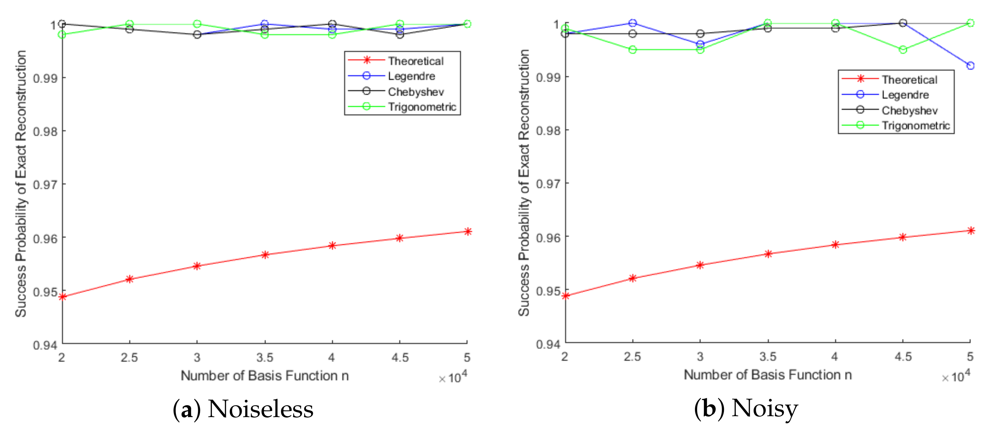
4.2. The Verification of Recovery Guarantee and Success Probability of OMP Algorithm

In this subsection, for the two cases of sampled data with and without noise, we take the uniformly bounded orthonormal systems in Section 4.1 as examples to verify the validity of the recovery guarantees and the lower bounds of the success probability given by Theorem 2 and Theorem 4, respectively. Here, the sparsity $s=5$ and $s=10$, the parameter $p=0.2,0.3$, and $0.4$, and the noise bound $\epsilon ={10}^{-5}$ are taken, respectively. The main steps of this experiment are as follows:

Step 1: Randomly generate an n-dimensional s-sparse coefficient vector $\mathbf{c}\in {\mathbb{R}}^n$ with a support set ${\Lambda }_s$.

Step 2: Taking the three types of uniformly bounded orthonormal system mentioned in Section 4.1 as examples, according to the corresponding probability measure, randomly select m sampling points ${\left\{x_i\right\}}_{i=1}^m$ on corresponding domain.

Step 3: Generate $b_i=g\left(x_i\right)={\sum }_{j\in \Lambda }{c}_j{\varphi }_j\left(x_i\right)$ or $b_i=(1/\sqrt{m})g\left(x_i\right)+$${ϵ}_i$.

Step 4: Use OMP to solve model (3) or (16).

Step 5: Compare the obtained results with the original coefficient vector and polynomial.

According to Theorem 2 and Theorem 4, we calculate the lower bounds of the number of sampling points m required for the three types of uniformly bounded orthonormal systems with different numbers of basis functions n and parameters p, which are the recovery guarantees for OMP to exactly reconstruct sparse polynomials. The recovery guarantees for the cases of $s=5$ and $s=10$ are shown in

Table 1. The lower bound of the number of sampling points m for the three types of the uniformly bounded orthonormal system when the sparsity $s=5$.

n	Lower Bound of the Number of Sampling Points m
	Preconditioned Legendre			Chebyshev			Trigonometric
p	0.2	0.3	0.4	0.2	0.3	0.4	0.2	0.3	0.4
5000	3748	3918	4089	2499	2612	2726	1250	1306	1363
10,000	4053	4237	4421	2702	2825	2948	1351	1413	1474
15,000	4231	4424	4616	2821	2949	3078	1411	1475	1539
20,000	4358	4556	4754	2906	3038	3170	1453	1519	1585
25,000	4456	4659	4861	2971	3106	3241	1486	1553	1621
30,000	4536	4743	4949	3024	3162	3299	1512	1581	1650
35,000	4604	4814	5023	3070	3209	3349	1535	1605	1675
40,000	4663	4875	5087	3109	3250	3391	1555	1625	1696
45,000	4715	4929	5143	3143	3286	3429	1572	1643	1715
50,000	4761	4978	5194	3174	3319	3463	1587	1660	1731

and

Table 2. The lower bound of the number of sampling points m for the three types of the uniformly bounded orthonormal system when the sparsity $s=10$.

n	Lower Bound of the Number of Sampling Points m
	Preconditioned Legendre			Chebyshev			Trigonometric
p	0.2	0.3	0.4	0.2	0.3	0.4	0.2	0.3	0.4
20,000	17,431	18,223	19,015	11,621	12,149	12,677	5811	6075	6339
25,000	17,823	18,634	19,444	11,882	12,423	12,963	5941	6212	6482
30,000	18,144	18,969	19,794	12,096	12,646	13,196	6048	6323	6589
35,000	18,416	19,253	20,090	12,277	12,835	13,393	6139	6418	6697
40,000	18,615	19,498	20,346	12,434	12,999	13,564	6217	6500	6782
45,000	18,858	19,715	20,572	12,572	13,144	13,715	6286	6572	6858
50,000	19,043	19,909	20,774	12,696	13,273	13,850	6348	6637	6925

, respectively.

The first column of Table 1 and Table 2 denotes the number of basis functions n, and the remaining columns denote the lower bound of the number of sampling points m required for different constants p at sparsity $s=5$ and $s=10$ for the three types of the uniformly bounded orthonormal systems, respectively. From Table 1 and Table 2, it is easy to see that the lower bound of the number of sampling points m increases with the increase of that of basis functions n, but the growth rate of the former is much smaller than the latter, and for the same n and s, the larger the parameter p is, the larger the lower bound of the number of sampling points m is. In addition, for the same number of basis functions n, sparsity s, and parameter p, the recovery guarantee of the trigonometric polynomial system is the smallest.

Next, for the sparse polynomials generated by the three types of uniformly bounded orthonormal system mentioned before, we take the number of basis functions n and sampling points m given in Table 1 and Table 2, and we solve model (3) by OMP for 1000 independent repeated experiments and record the frequency of exact reconstruction as the actual success probability of OMP. It is clear that for different number of basis functions n and parameter p, the theoretical success probability is $1-n^{-p}$. For the two cases of sampled data with and without noise, Figure 1, Figure 2, Figure 3, Figure 4, Figure 5 and Figure 6 show the comparison between the theoretical and actual success probability for OMP to exactly reconstruct the three types of sparse polynomials for different numbers of basis functions n, parameter p, and sparsity s.

From Figure 1, Figure 2, Figure 3, Figure 4, Figure 5 and Figure 6, it is easy to see that the theoretical success probability (red line) of OMP to reconstruct the three types of sparse polynomials with different parameters p gradually increases and tends to the actual success probability as the number of basis functions n increases, and the actual success probability is higher than the theoretical success probability in both noisy and noiseless cases. When the number of basis functions n is the same, the theoretical success probability also increases with the increase of parameter p, which illustrates the correctness and validity of the conclusions of Theorem 2 and Theorem 4. In addition, Figure 1, Figure 2, Figure 3, Figure 4, Figure 5 and Figure 6 also show that when the sampled data contain noise of magnitude $\epsilon ={10}^{-5}$, the success probability for OMP is comparable to that of the case when the sampled data do not contain noise, which also illustrates the robustness of OMP.

4.3. Verification of the Accuracy of the Reconstruction Error Estimation When Sampled Data Contain Noise

In this subsection, for the sampled data containing noise, we verify the accuracy of the reconstruction error estimation for the sparse coefficient vector. The number of basis functions n, sampling points m, and the noise bound are still taken as Table 1, Table 2, and $\epsilon ={10}^{-5}$, respectively. The experimental procedure is similar to that in Section 4.2, where we still perform 1000 independent repeated experiments by using OMP to reconstruct the three types of sparse polynomials. Different from the experiments in Section 4.2, we randomly generate a noise vector $ϵ$ with ${\parallel ϵ\parallel }_2\le \epsilon$ and record the values of constant C and the real noise bound $\tilde{\epsilon }={\parallel ϵ\parallel }_2$ when OMP succeeds. For the two cases of sparsity $s=5$ and $s=10$, the average reconstruction error and the upper bound of it are shown in

Table 3. The actual reconstruction error and the upper bound of reconstruction error for OMP to recover the coefficient vectors of the three types of sparse polynomials, $s=5$.

n	p	Preconditioned Legendre		Chebyshev		Trigonometric
		Upper Bound	Error	Upper Bound	Error	Upper Bound	Error
20,000	0.2	5.9420 $\times {10}^{-6}$	1.8612 $\times {10}^{-7}$	5.9226 $\times {10}^{-6}$	2.3162 $\times {10}^{-7}$	5.9950 $\times {10}^{-6}$	3.3156 $\times {10}^{-7}$
	0.3	5.9346 $\times {10}^{-6}$	1.8189 $\times {10}^{-7}$	5.9223 $\times {10}^{-6}$	2.2176 $\times {10}^{-7}$	5.9860 $\times {10}^{-6}$	3.2614 $\times {10}^{-7}$
	0.4	5.9347 $\times {10}^{-6}$	1.7854 $\times {10}^{-7}$	5.9195 $\times {10}^{-6}$	2.1832 $\times {10}^{-7}$	5.9863 $\times {10}^{-6}$	3.1439 $\times {10}^{-7}$
40,000	0.2	5.9415 $\times {10}^{-6}$	1.7713 $\times {10}^{-7}$	5.9179 $\times {10}^{-6}$	2.2273 $\times {10}^{-7}$	5.9893 $\times {10}^{-6}$	3.2066 $\times {10}^{-7}$
	0.3	5.9288 $\times {10}^{-6}$	1.7402 $\times {10}^{-7}$	5.9160 $\times {10}^{-6}$	2.1478 $\times {10}^{-7}$	5.9808 $\times {10}^{-6}$	3.1279 $\times {10}^{-7}$
	0.4	5.9308 $\times {10}^{-6}$	1.7416 $\times {10}^{-7}$	5.9150 $\times {10}^{-6}$	2.1179 $\times {10}^{-7}$	5.9810 $\times {10}^{-6}$	3.0817 $\times {10}^{-7}$
50,000	0.2	5.9307 $\times {10}^{-6}$	1.7897 $\times {10}^{-7}$	5.9201 $\times {10}^{-6}$	2.2058 $\times {10}^{-7}$	5.9869 $\times {10}^{-6}$	3.1696 $\times {10}^{-7}$
	0.3	5.9301 $\times {10}^{-6}$	1.7361 $\times {10}^{-7}$	5.9149 $\times {10}^{-6}$	2.1592 $\times {10}^{-7}$	5.9777 $\times {10}^{-6}$	3.0936 $\times {10}^{-7}$
	0.4	5.9258 $\times {10}^{-6}$	1.7054 $\times {10}^{-7}$	5.9106 $\times {10}^{-6}$	2.0830 $\times {10}^{-7}$	5.9787 $\times {10}^{-6}$	3.0729 $\times {10}^{-7}$

and

Table 4. The actual reconstruction error and the upper bound of reconstruction error for OMP to recover the coefficient vectors of the three types of sparse polynomials, $s=10$.

n	p	Preconditioned Legendre		Chebyshev		Trigonometric
		Upper Bound	Error	Upper Bound	Error	Upper Bound	Error
20,000	0.2	5.9530 $\times {10}^{-6}$	1.3369 $\times {10}^{-7}$	5.8490 $\times {10}^{-6}$	1.1562 $\times {10}^{-7}$	5.9638 $\times {10}^{-6}$	2.2914 $\times {10}^{-7}$
	0.3	5.9462 $\times {10}^{-6}$	1.3542 $\times {10}^{-7}$	5.8489 $\times {10}^{-6}$	1.1564 $\times {10}^{-7}$	5.9590 $\times {10}^{-6}$	2.3235 $\times {10}^{-7}$
	0.4	5.9176 $\times {10}^{-6}$	1.2626 $\times {10}^{-7}$	5.8494 $\times {10}^{-6}$	1.0587 $\times {10}^{-7}$	5.9622 $\times {10}^{-6}$	2.2498 $\times {10}^{-7}$
40,000	0.2	5.9412 $\times {10}^{-6}$	1.2278 $\times {10}^{-7}$	5.8480 $\times {10}^{-6}$	1.0481 $\times {10}^{-7}$	5.9567 $\times {10}^{-6}$	2.2734 $\times {10}^{-7}$
	0.3	5.9063 $\times {10}^{-6}$	1.2800 $\times {10}^{-7}$	5.8443 $\times {10}^{-6}$	1.1113 $\times {10}^{-7}$	5.9534 $\times {10}^{-6}$	2.1706 $\times {10}^{-7}$
	0.4	5.9037 $\times {10}^{-6}$	1.2962 $\times {10}^{-7}$	5.8419 $\times {10}^{-6}$	9.9783 $\times {10}^{-8}$	5.9500 $\times {10}^{-6}$	2.1759 $\times {10}^{-7}$
50,000	0.2	5.9082 $\times {10}^{-6}$	1.3328 $\times {10}^{-7}$	5.8454 $\times {10}^{-6}$	1.0770 $\times {10}^{-7}$	5.9634 $\times {10}^{-6}$	2.2618 $\times {10}^{-7}$
	0.3	5.9097 $\times {10}^{-6}$	1.2813 $\times {10}^{-7}$	5.8436 $\times {10}^{-6}$	1.0537 $\times {10}^{-7}$	5.9548 $\times {10}^{-6}$	2.1822 $\times {10}^{-7}$
	0.4	5.9085 $\times {10}^{-6}$	1.3133 $\times {10}^{-7}$	5.8403 $\times {10}^{-6}$	1.0581 $\times {10}^{-7}$	5.9489 $\times {10}^{-6}$	2.1657 $\times {10}^{-7}$

when the parameter $p=0.2$, $0.3$, and $0.4$ and OMP succeeds.

The columns of ‘upper bound’ in Table 3 and Table 4 are the estimation of the upper bound of the reconstruction error, i.e., $C·\tilde{\epsilon }$, and the columns of ‘error’ mean the average reconstruction error when OMP succeeds, i.e., $\parallel \mathbf{c}-\tilde{\mathbf{c}}{\parallel }_2$. From Table 3 and Table 4, it is easy to see that for the three types of sparse polynomials, with different numbers of basis functions n and parameters p, all the upper bounds of the reconstruction errors are larger than the average reconstruction errors, which shows the correctness of the conclusion in Theorem 4.

4.4. Verification of the Accuracy of OMP to Recover Coefficient Vectors When Sampled Data Contain Noise

The case of sampled data $g\left(x_i\right),i=1,2,\cdots ,m$ with noise can be regarded as the case that the coefficient vector contains noise, which can be expressed as

$$\tilde{g}\left(x_i\right)=\sum _{j=1}^n{c}_j\frac{{\varphi }_j\left(x_i\right)}{\parallel {\Phi }_j{\parallel }_2}+{\epsilon }_i=\sum _{j=1}^n{\widehat{c}}_j\frac{{\varphi }_j\left(x_i\right)}{\parallel {\Phi }_j{\parallel }_2},i=1,2,\cdots ,m.$$

It can be written in the matrix vector form as

$$\widehat{\mathbf{b}}=\tilde{\Phi }\widehat{\mathbf{c}},$$

where $\tilde{\Phi }$ and $\widehat{\mathbf{b}}=\tilde{\mathbf{b}}$ are given as (14) and (15), respectively, and the vector $\widehat{\mathbf{c}}={\left[{\widehat{c}}_1,\cdots ,{\widehat{c}}_n\right]}^{\top }\in {\mathbb{R}}^{n\times 1}$. At this point, only s main term in the vector $\widehat{\mathbf{c}}$ has a large absolute value, and the absolute values of the remaining terms are small. Therefore, in this subsection, for the case of coefficient vector with noise, we apply OMP to recover the noisy coefficient vector $\widehat{\mathbf{c}}$ and then verify the recovery effect of OMP. In this experiment, the noise bound is still taken as $\epsilon ={10}^{-5}$, and the number of basis functions n and sampling points m are still taken as those in Table 1 and Table 2 for $s=5$ and $s=10$, respectively. We solve model (16) by OMP for 1000 independent repeated experiments and record the actual error $\parallel \widehat{\mathbf{c}}-\tilde{\mathbf{c}}{\parallel }_2$ when OMP succeeds. The average actual errors of $s=5$ and $s=10$ are shown in

Table 5. The average actual error for OMP to recover the coefficients of the three types of sparse polynomials, $s=5$.

n	p	Actual Error
		Preconditioned Legendre	Chebyshev	Trigonometric
20,000	0.2	5.7726 $\times {10}^{-6}$	5.7793 $\times {10}^{-6}$	5.7755 $\times {10}^{-6}$
	0.3	5.7735 $\times {10}^{-6}$	5.7718 $\times {10}^{-6}$	5.7818 $\times {10}^{-6}$
	0.4	5.7751 $\times {10}^{-6}$	5.7731 $\times {10}^{-6}$	5.7799 $\times {10}^{-6}$
40,000	0.2	5.7864 $\times {10}^{-6}$	5.7733 $\times {10}^{-6}$	5.7849 $\times {10}^{-6}$
	0.3	5.7796 $\times {10}^{-6}$	5.7784 $\times {10}^{-6}$	5.7782 $\times {10}^{-6}$
	0.4	5.7814 $\times {10}^{-6}$	5.7792 $\times {10}^{-6}$	5.7792 $\times {10}^{-6}$
50,000	0.2	5.7791 $\times {10}^{-6}$	5.7772 $\times {10}^{-6}$	5.7792 $\times {10}^{-6}$
	0.3	5.7802 $\times {10}^{-6}$	5.7801 $\times {10}^{-6}$	5.7798 $\times {10}^{-6}$
	0.4	5.7773 $\times {10}^{-6}$	5.7774 $\times {10}^{-6}$	5.7840 $\times {10}^{-6}$

and

Table 6. The average actual error for OMP to recover the coefficients of the three types of sparse polynomials, $s=10$.

n	p	Actual Error
		Preconditioned Legendre	Chebyshev	Trigonometric
20,000	0.2	5.7782 $\times {10}^{-6}$	5.7756 $\times {10}^{-6}$	5.7753 $\times {10}^{-6}$
	0.3	5.7681 $\times {10}^{-6}$	5.7793 $\times {10}^{-6}$	5.7703 $\times {10}^{-6}$
	0.4	5.7734 $\times {10}^{-6}$	5.7900 $\times {10}^{-6}$	5.7753 $\times {10}^{-6}$
40,000	0.2	5.7788 $\times {10}^{-6}$	5.7762 $\times {10}^{-6}$	5.7760 $\times {10}^{-6}$
	0.3	5.7771 $\times {10}^{-6}$	5.7810 $\times {10}^{-6}$	5.7816 $\times {10}^{-6}$
	0.4	5.7781 $\times {10}^{-6}$	5.7659 $\times {10}^{-6}$	5.7760 $\times {10}^{-6}$
50,000	0.2	5.7765 $\times {10}^{-6}$	5.7721 $\times {10}^{-6}$	5.7711 $\times {10}^{-6}$
	0.3	5.7734 $\times {10}^{-6}$	5.7763 $\times {10}^{-6}$	5.7856 $\times {10}^{-6}$
	0.4	5.7765 $\times {10}^{-6}$	5.7808 $\times {10}^{-6}$	5.7711 $\times {10}^{-6}$

, respectively.

The first column of Table 5 and Table 6 indicates the number of basis functions, the second column indicates the value of parameter p, and the remaining columns indicate the average actual error when OMP succeeds. From Table 5 and Table 6, it is easy to see that when OMP succeeds, the actual error of its recovery is smaller than the error bound $\epsilon$, which indicates the accuracy of OMP in recovering the noisy coefficient vector, and also shows the noise resistance of OMP.

5. Conclusions

The main work of this paper is to give the sufficient conditions for OMP to reconstruct sparse polynomials generated by uniformly bounded orthonormal systems in both cases of sampled data with and without noise, and give the recovered error for the sparse coefficient vectors when the sampled data contain noise. The work in this paper can be regarded as a generalization of the study of OMP to reconstruct sparse trigonometric polynomials in [21].

For the structured random matrix generated by a uniformly bounded orthonormal system and random sampling points, a more accurate estimation for the upper bound of the mutual coherence of this matrix is given firstly in this paper. Then, for both cases of sampled data with and without noise, when the measurement matrix is a structured random matrix, more relaxed sufficient conditions for OMP to recover sparse coefficient vectors with high probability are given by the mutual coherence of the measurement matrix, which further relax the condition $\mu (\Phi )<1/(2s-1)$ given in [9,19]. Meanwhile, the requirement on the sparse coefficient vector for OMP to exactly find the positions of nonzero elements is given when the sampled data contain noise. Finally, combining the results of the above two parts, it is proved that regardless of whether the sampled data contain noise or not, when the number of sampling points satisfies $m\sim s^{2}lnn$, OMP can reconstruct general sparse polynomials with probability at least $1-n^{-p}$ in both cases. Furthermore, with a simple calculation, the fact that reconstruction error between the original and recovered coefficient vector can be controlled by the noise bound is also illustrated in this paper. In addition, the research methods and conclusions of this paper can be extended to the study of multivariate sparse polynomial reconstruction problems.

However, it is easy to see from the experiments in Section 4.2 that the actual success probability of OMP is higher than the theoretical success probability, which indicates that the recovery guarantee given in this paper is not optimal. Perhaps some more advanced probability tools can be used to give a more accurate upper bound estimation for the mutual coherence of the measurement matrix, which in turn can further optimize the recovery guarantee and the success probability for OMP.

References

1. Foucart, S.; Lai, M.-J. Sparsest solutions of underdetermined linear systems via q-minimization for 0 < q ≤ 1. Appl. Comput. Harmon. Anal. 2009, 26, 395–407. [Google Scholar]
2. Rauhut, H.; Ward, R. Sparse Legendre expansions via l(1)-minimization. J. Approx. Theory. 2012, 164, 517–533. [Google Scholar] [CrossRef] [Green Version]
3. Rauhut, H.; Ward, R. Interpolation via weighted 1 minimization. Appl. Comput. Harmon. Anal. 2016, 40, 321–351. [Google Scholar] [CrossRef]
4. Xu, Z. Deterministic sampling of sparse trigonometric polynomials. J. Complex. 2011, 27, 133–140. [Google Scholar] [CrossRef] [Green Version]
5. Xu, Z.; Zhou, T. On Sparse Interpolation and the Design of Deterministic interpolation points. SIAM J. Sci. Comput. 2014, 36, 1752–1769. [Google Scholar] [CrossRef] [Green Version]
6. Ho, L.; Schaeffer, H.; Tran, G.; Ward, R. Recovery guarantees for polynomial coefficients from weakly dependent data with outliers. J. Approx. Theory 2020, 259, 105472. [Google Scholar] [CrossRef]
7. Candes, E.J.; Romberg, J.; Tao, T. Robust uncertainty principles: Exact signal reconstruction from highly incomplete frequency information. IEEE Trans. Inf. Theory 2006, 52, 489–509. [Google Scholar] [CrossRef] [Green Version]
8. Xu, Z. Compressed sensing: A survey. Sci. Sin. Math. 2012, 42, 865–877. (In Chinese) [Google Scholar] [CrossRef]
9. Tropp, J.A. Greed is good: Algorithmic results for sparse approximation. IEEE Trans. Inf. Theory 2004, 50, 2231–2242. [Google Scholar] [CrossRef] [Green Version]
10. Feng, R.; Huang, A.; Lai, M.J.; Shen, Z. Reconstruction of Sparse Polynomials via Quasi-Orthogonal Matching Pursuit Method. J. Comput. Math. 2021. [Google Scholar] [CrossRef]
11. Huang, A.; Feng, R.; Zheng, S. Recovery Guarantee for Orthogonal Matching Pursuit Method to Reconstruct Sparse Polynomials. Numer. Math. Theor. Meth. Appl. 2022, 15, 793–818. [Google Scholar] [CrossRef]
12. Lin, J.; Li, S. Nonuniform support recovery from noisy random measurements by orthogonal matching pursuit. J. Approx. Theory 2013, 165, 20–40. [Google Scholar] [CrossRef] [Green Version]
13. Fornasier, M. Theoretical Foundations and Numerical Methods for Sparse Recovery; DE GRUYTER: Berlin, Germany, 2010. [Google Scholar]
14. Mo, Q.; Shen, Y. A remark on the restricted isometry property in orthogonal matching pursuit. IEEE Trans. Inf. Theory 2012, 58, 3654–3656. [Google Scholar] [CrossRef] [Green Version]
15. Wang, J.; Shim, B. On the recovery limit of sparse signals using orthogonal matching pursuit. IEEE Trans. Signal Process 2012, 60, 4973–4976. [Google Scholar] [CrossRef]
16. Mo, Q. A sharp restricted isometry constant bound of orthogonal matching pursuit. arXiv 2015, arXiv:1501.01708. [Google Scholar]
17. Wen, J.; Zhou, Z.; Wang, J.; Tang, X.; Mo, Q. A sharp condition for exact support recovery with orthogonal matching pursuit. IEEE Trans. Signal Process 2017, 65, 1370–1382. [Google Scholar] [CrossRef] [Green Version]
18. Tropp, J.A.; Gilbert, A.C. Signal recovery from random measurements via orthogonal matching pursuit. IEEE Trans. Inf. Theory 2007, 53, 4655–4666. [Google Scholar] [CrossRef] [Green Version]
19. Cai, T.T.; Wang, L. Orthogonal matching pursuit for sparse signal recovery with noise. IEEE Trans. Inf. Theory 2011, 57, 4680–4688. [Google Scholar] [CrossRef]
20. Cai, T.T.; Wang, L.; Xu, G. Stable recovery of sparse signals and an oracle inequality. IEEE Trans. Inf. Theory 2010, 56, 3516–3522. [Google Scholar] [CrossRef]
21. Kunis, S.; Rauhut, H. Random sampling of sparse trigonometric polynomials ii: Orthogonal matching pursuit versus basis pursuit. Found. Comput. Math. 2008, 6, 737–763. [Google Scholar] [CrossRef] [Green Version]
22. Random sampling of sparse trigonometric polynomials. Appl. Comput. Harmon. Anal. 2007, 22, 16–42. [CrossRef] [Green Version]
23. Xu, Z.; Zhou, T. A gradient-enhanced 1 approach for the recovery of sparse trigonometric polynomials. Commun. Comput. Phys. 2018, 24, 286–308. [Google Scholar] [CrossRef]
24. Davis, G.; Mallat, S.; Avellaneda, M. Adaptive greedy approximations. Constr. Approx. 1997, 13, 57–98. [Google Scholar] [CrossRef]
25. Foucart, S.; Rauhut, H. A Mathematical Introduction to Compressive Sensing; Springer: New York, NY, USA, 2013. [Google Scholar]
26. Dunkl, C.F.; Xu, Y. Orthogonal Polynomials of Several Variables; Cambridge University Press: Cambridge, UK, 2001. [Google Scholar]
27. Rivlin, T.J. The Chebyshev Polynomials; Dover: Mignola, NY, USA, 1974. [Google Scholar]
28. Zygmund, A. Trigonometric Series; Cambridge University Press: Cambridge, UK, 1959. [Google Scholar]
Figure 1. Comparison between the theoretical and actual success probability of OMP to reconstruct three types of sparse polynomials when the sampled data are noiseless and noisy, s = 5 , p = 0.2 .
Mathematics 10 03703 g001
Figure 2. Comparison between the theoretical and actual success probability of OMP to reconstruct three types of sparse polynomials when the sampled data are noiseless and noisy, s = 5 , p = 0.3 .
Mathematics 10 03703 g002
Figure 3. Comparison between the theoretical and actual success probability of OMP to reconstruct three types of sparse polynomials when the sampled data are noiseless and noisy, s = 5 , p = 0.4 .
Mathematics 10 03703 g003
Figure 4. Comparison between the theoretical and actual success probability of OMP to reconstruct three types of sparse polynomials when the sampled data are noiseless and noisy, s = 10 , p = 0.2 .
Mathematics 10 03703 g004
Figure 5. Comparison between the theoretical and actual success probability of OMP to reconstruct three types of sparse polynomials when the sampled data are noiseless and noisy, s = 10 , p = 0.3 .
Mathematics 10 03703 g005
Figure 6. Comparison between the theoretical and actual success probability of OMP to reconstruct three types of sparse polynomials when the sampled data are noiseless and noisy, s = 10 , p = 0.4 .
Mathematics 10 03703 g006