A Boundary Shape Function Method for Computing Eigenvalues and Eigenfunctions of Sturm–Liouville Problems

Abstract

In the paper, we transform the general Sturm–Liouville problem (SLP) into two canonical forms: one with the homogeneous Dirichlet boundary conditions and another with the homogeneous Neumann boundary conditions. A boundary shape function method (BSFM) was constructed to solve the SLPs of these two canonical forms. Owing to the property of the boundary shape function, we could transform the SLPs into an initial value problem for the new variable with initial values that were given definitely. Meanwhile, the terminal value at the right boundary could be entirely determined by using a given normalization condition for the uniqueness of the eigenfunction. In such a manner, we could directly determine the eigenvalues as the intersection points of an eigenvalue curve to the zero line, which was a horizontal line in the plane consisting of the zero values of the target function with respect to the eigen-parameter. We employed a more delicate tuning technique or the fictitious time integration method to solve an implicit algebraic equation for the eigenvalue curve. We could integrate the Sturm–Liouville equation using the given initial values to obtain the associated eigenfunction when the eigenvalue was obtained. Eight numerical examples revealed a great advantage of the BSFM, which easily obtained eigenvalues and eigenfunctions with the desired accuracy.

1. Introduction

During 1836–1837, Sturm and Liouville created a new subject in the mathematical analysis of second-order ordinary differential equations (ODEs) with the homogeneous Sturm–Liouville boundary conditions. It is known as the Sturm–Liouville theory nowadays, and deals with the Sturm–Liouville problem (SLP):

$$-{\left(p\left(x\right)u^{\prime }\left(x\right)\right)}^{\prime }+q\left(x\right)u\left(x\right)=\lambda \omega \left(x\right)u\left(x\right), x\in \left(a,b\right),$$

(1)

$$hu\left(a\right)-p\left(a\right)u^{\prime }\left(a\right)=0, Hu\left(b\right)+p\left(b\right)u^{\prime }\left(b\right)=0,$$

(2)

where $p\left(x\right)>0$ and $\omega \left(x\right)>0$ are strictly positive functions of $x$ in a finite interval $\left[a, b\right]$ and $\lambda$ is a constant parameter. The two-point boundary value problem (1) and (2) is a regular SLP that allows nontrivial solutions only for specific values of $\lambda$, which are known as the eigenvalues. Only in a few cases can the eigenvalues be obtained analytically by solving algebraic equations; however, we do not even have explicit algebraic equations to solve $\lambda$ for most cases.

SLPs are essential in partial differential equations, vibrations in continuum mechanics, heat conduction problems, the Schrödinger equation, the transport of microwaves, the Lax pair of the Korteweg–De Vries equation, and fractional derivative problems [1,2,3,4], etc. Many numerical method, such as the residuals–collocation method [5], Chebyshev collocation method [6,7], shooting method [8], exponentially fitted Numerov method [9], differential quadrature method [10,11], Sinc–Galerkin method [12], Adomian decomposition method [13], homotopy analysis method [14], and variational iteration method [15] have been developed in the past several decades to solve SLPs. These methods have been widely applied and efficient and accurate codes have been developed. On the other hand, the modified shooting methods were developed by Ghelardoni and Gheri [16] and Liu [17,18]. Compared with the corrected Numerov’s method in recent years, competitive results have been obtained by applying symmetric boundary value methods [19,20] and using high-order difference schemes [21].

This paper’s main focus was to develop the boundary shape function (BSF) to solve SLPs by automatically satisfying the boundary conditions. First, the idea of the boundary shape function proposed by Liu and Chang [22] was applied to find the periodic solution of nonlinear jerk equations. Then, some problems such as the optimal control problems of nonlinear Duffing oscillators and the boundary value problem (BVP) with different boundary conditions were addressed by the BSF. New methods based on the BSF were developed to address the SLPs that were easy to formulate and implement. There are various numerical methods to approximate the eigenvalue and the corresponding eigenfunction. The present technique used the BSF to transform the SLP to the initial value problem (IVP), which was drastically different from the Lie-group shooting method developed by Liu [17]. This new method did not need to find the missing initial values via the shooting technique; the difference will be pointed out below.

The paper is arranged as follows. Two main theorems are proven in Section 2 for the SLP with the homogeneous Sturm–Liouville boundary conditions. Here, we developed two novel transformation methods to derive two canonical forms that transformed the general SLP to those with homogeneous Dirichlet and Neumann boundary conditions. In Section 3, we transform the SLP with the Dirichlet boundary conditions to an IVP for a new variable, which guaranteed that the Dirichlet boundary conditions for $y\left(x\right)$ could be satisfied automatically. In the transformed IVP for $z\left(x\right)$, an unknown constant $z\left(b\right)$ appeared that is yet to be determined. In Section 4, we derive $z\left(b\right)$ in terms of the initial values for $z\left(x\right)$ and a normalized value $A_0$ given in $y^{\prime }\left(a\right)=A_0$ for the uniqueness of the eigenfunction $y\left(x\right)$, which could avoid the iteration to determine $z\left(b\right)$. The numerical algorithm based on the boundary shape function method (BSFM) is developed in Section 5. Numerical examples with the homogeneous Dirichlet boundary conditions are given in Section 6 that verify the new results and algorithms. In Section 7, the BSFM is derived to solve the SLP with the homogeneous Neumann boundary conditions. In Section 8, several examples are given of homogeneous Sturm–Liouville boundary conditions. Finally, some conclusions are presented in Section 9.

2. Sturm–Liouville Boundary Conditions

It is well known that the eigenvalues satisfy the relation:

$${\lambda }_0<{\lambda }_1<\dots {\lambda }_n,$$

(3)

and the eigenfunction corresponding to an eigenvalue ${\lambda }_n$ has $n$ intersections with the x-axis inside the interval $x\in \left(a,b\right)$. Moreover, since for any given eigenvalue it is possible to compute an infinite number of eigenfunctions, in general, a normalization condition in the form ${\int }_a^b{u}^2\left(x\right)dx=1$ is required for the uniqueness of $u\left(x\right)$. The computation of $\lambda$ and $u\left(x\right)$ traditionally has been quite a challenging task. We will show that inexpensive computing that evaluates $\lambda$ via a direct solution of the differential Equation (1) is feasible.

For the general SLP of Equations (1) and (2), we supposed that $u\left(a\right)\ne 0$, $u^{\prime }\left(a\right)\ne 0$, $u\left(b\right)\ne 0$, and $u^{\prime }\left(b\right)\ne 0$. We transformed them into two canonical forms with the Dirichlet and Neumann homogeneous boundary conditions, respectively, and then proposed a BSFM for determining the eigenvalues and finding the corresponding eigenfunctions.

2.1. Transforming to Neumann-Type Boundary Conditions

In Equations (1) and (2), suppose that $h\ne 0$ and $H\ne 0$ such that the coefficients preceding $u\left(a\right)$ and $u\left(b\right)$ can be set equal to one. When letting ${\mu }_1=-p\left(a\right)/h$ and ${\mu }_2=-p\left(b\right)/H$, we may need to prove the following result.

Theorem 1.

For the SLP with the Sturm–Liouville type boundary conditions:

$$-{\left(p\left(x\right)u^{\prime }\left(x\right)\right)}^{\prime }+q\left(x\right)u\left(x\right)=\lambda \omega \left(x\right)u\left(x\right), x\in \left(a,b\right),$$

(4)

$$u\left(a\right)+{\mu }_1{u}^{\prime }\left(a\right)=0, ub+{\mu }_2{u}^{\prime }\left(b\right)=0,$$

(5)

where λ is an eigen-parameter. If the following condition is satisfied:

$$\frac{{\mu }_2-{\mu }_1}{b-a}=1,$$

(6)

then Equations (4) and (5) can be transformed into the Neumann-type SLP:

$$-{\left[\frac{p\left(x\right)y^{\prime }\left(x\right)}{{\left(x+{\mu }_1-a\right)}^2}\right]}^{\prime }+\left[\frac{p^{\prime }\left(x\right)}{{\left(x+{\mu }_1-a\right)}^3}-\frac{2p\left(x\right)}{{\left(x+{\mu }_1-a\right)}^4}+\frac{q\left(x\right)}{{\left(x+{\mu }_1-a\right)}^2}\right]y\left(x\right)=\frac{\lambda \omega \left(x\right)y\left(x\right)}{{\left(x+{\mu }_1-a\right)}^2},$$

(7)

$$y^{\prime }\left(a\right)=0, y^{\prime }\left(b\right)=0.$$

(8)

The relation between $u\left(x\right)$ and $y\left(x\right)$ is given as:

$$y\left(x\right)=\left(x+{\mu }_1-a\right)u\left(x\right).$$

(9)

Proof. 

Let:

$$y^{\prime }\left(x\right)=\left[1-\frac{x-a}{b-a}\right]\left[u\left(x\right)+{\mu }_1{u}^{\prime }\left(x\right)\right]+\frac{x-a}{b-a}\left[u\left(x\right)+{\mu }_2{u}^{\prime }\left(x\right)\right].$$

(10)

It is apparent that the Neumann boundary conditions in Equation (8) follow from Equation (5) upon using the above equation. It follows from Equation (10) that:

$$y^{\prime }\left(x\right)=u\left(x\right)+\left[{\mu }_1+\left({\mu }_2-{\mu }_1\right)\frac{x-a}{b-a}\right]u^{\prime }\left(x\right).$$

(11)

If condition (6) holds, Equation (11) reduces to:

$$y^{\prime }\left(x\right)=u\left(x\right)+\left(x+{\mu }_1-a\right)u^{\prime }\left(x\right)={\left[\left(x+{\mu }_1-a\right)u\left(x\right)\right]}^{\prime }.$$

(12)

Thus, $y\left(x\right)=\left(x+{\mu }_1-a\right)u\left(x\right)$ in Equation (9) is proved. Inserting Equation (9) and its first and second differentials into Equation (4), we can derive:

$$-{\left(p\left(x\right)y^{\prime }\left(x\right)\right)}^{\prime }+\frac{2p\left(x\right)y^{\prime }\left(x\right)}{\left(x+{\mu }_1-a\right)}+\left[\frac{p^{\prime }\left(x\right)}{\left(x+{\mu }_1-a\right)}-\frac{2p\left(x\right)}{{\left(x+{\mu }_1-a\right)}^2}+q\left(x\right)\right]y\left(x\right)=\lambda \omega \left(x\right)y\left(x\right),$$

(13)

which, when multiplied by $1/{\left(x+{\mu }_1-a\right)}^2$ on both sides, can lead to Equation (7). □

Motivated by Theorem 1, we generalized it to the Sturm–Liouville type boundary conditions without needing the constraint ${\mu }_2-{\mu }_1=b-a$. For this purpose, we sought a function $F\left(x\right)$ in:

$$y\left(x\right)=F\left(x\right)u\left(x\right),$$

(14)

so that the Sturm–Liouville type boundary conditions in Equation (5) with $u^{\prime }\left(a\right)\ne 0$ and $u^{\prime }\left(b\right)\ne 0$ were transformed to:

$$y^{\prime }\left(a\right)=F^{\prime }\left(a\right)u\left(a\right)+F\left(a\right)u^{\prime }\left(a\right)=\left[F\left(a\right)-{\mu }_1{F}^{\prime }\left(a\right)\right]u^{\prime }\left(a\right)=0\Rightarrow F\left(a\right)-{\mu }_1{F}^{\prime }\left(a\right)=0,$$

(15)

$$y^{\prime }\left(b\right)=F^{\prime }\left(b\right)u\left(b\right)+F\left(b\right)u^{\prime }\left(b\right)=\left[F\left(b\right)-{\mu }_2{F}^{\prime }\left(b\right)\right]u^{\prime }\left(b\right)=0\Rightarrow F\left(b\right)-{\mu }_2{F}^{\prime }\left(b\right)=0.$$

(16)

Through some manipulations, we can derive:

$$F\left(x\right)=\frac{1}{b-a}+\frac{x-a}{{\mu }_1\left(b-a\right)}+\frac{\left({\mu }_1-{\mu }_2+b-a\right){\left(x-a\right)}^2}{{\mu }_1\left(2{\mu }_2-b+a\right){\left(b-a\right)}^2},\mathrm{if} 2{\mu }_2-b+a\ne 0,$$

(17)

$$F\left(x\right)=\frac{1}{b-a}+\frac{x-a}{{\mu }_1\left(b-a\right)}+\frac{\left({\mu }_1-{\mu }_2+b-a\right){\left(x-a\right)}^3}{{\mu }_1\left(3{\mu }_2-b+a\right){\left(b-a\right)}^3},\mathrm{if} 2{\mu }_2-b+a=0.$$

(18)

Theorem 2. 

The SLP (4) and (5) with $u^{\prime }\left(a\right)\ne 0$ and $u^{\prime }\left(b\right)\ne 0$ in the Sturm–Liouville boundary conditions can be transformed to the Neumann-type boundary conditions:

$$-{\left[\frac{p\left(x\right)y^{\prime }\left(x\right)}{F^2\left(x\right)}\right]}^{\prime }+\left[\frac{p^{\prime }\left(x\right)F^{\prime }\left(x\right)+p\left(x\right)F^{″}\left(x\right)}{F^3\left(x\right)}-\frac{2p\left(x\right)F^{\prime }{\left(x\right)}^2}{F^4\left(x\right)}+\frac{q\left(x\right)}{F^2\left(x\right)}\right]y\left(x\right)=\frac{\lambda \omega \left(x\right)y\left(x\right)}{F^2\left(x\right)},$$

(19)

$$y^{\prime }\left(a\right)=0, y^{\prime }\left(b\right)=0,$$

(20)

where the relation between $u\left(x\right)$ and $y\left(x\right)$ is given by Equation (14) and $F\left(x\right)$ is given by Equations (17) or (18).

Proof. 

The Neumann boundary conditions in Equation (20) are given by Equations (15) and (16). By inserting Equation (14) and its first differential into Equation (4), we can derive:

$$-{\left(\frac{p\left(x\right)y^{\prime }\left(x\right)}{F\left(x\right)}\right)}^{\prime }+\frac{p\left(x\right)F^{\prime }\left(x\right)y^{\prime }}{F^2\left(x\right)}+{\left(\frac{p\left(x\right)F^{\prime }\left(x\right)}{F^2\left(x\right)}\right)}^{\prime }y+\frac{q\left(x\right)y}{F\left(x\right)}=\frac{\lambda \omega \left(x\right)y}{F\left(x\right)}.$$

(21)

When Equation (21) is divided by $F\left(x\right)$ on both sides and use:

$$-{\left(\frac{p\left(x\right)y^{\prime }}{F^2\left(x\right)}\right)}^{\prime }=-\frac{1}{F\left(x\right)}{\left(\frac{p\left(x\right)y^{\prime }}{F\left(x\right)}\right)}^{\prime }-\frac{p\left(x\right)y^{\prime }}{F\left(x\right)}{\left(\frac{1}{F\left(x\right)}\right)}^{\prime }=-\frac{1}{F\left(x\right)}{\left(\frac{p\left(x\right)y^{\prime }}{F\left(x\right)}\right)}^{\prime }+\frac{p\left(x\right)F^{\prime }\left(x\right)y^{\prime }}{F^3\left(x\right)},$$

we can change it to:

$$-{\left(\frac{p\left(x\right)y^{\prime }}{F^2\left(x\right)}\right)}^{\prime }+\frac{1}{F\left(x\right)}{\left(\frac{p\left(x\right)F^{\prime }\left(x\right)}{F^2\left(x\right)}\right)}^{\prime }y+\frac{q\left(x\right)y}{F^2\left(x\right)}=\frac{\lambda \omega \left(x\right)y}{F^2\left(x\right)}.$$

(22)

The expansion of the second term generates Equation (19). □

Note that Niessen and Zettl [23] developed a similar transformation ($y\left(x\right)=u\left(x\right)/f\left(x\right)$), where $f\left(x\right)$ is a solution of Equation (1) for some $\lambda$. The purpose was to transform the singular SLP with a singular nonoscillatory limit circle endpoint into a regular one. However, the present $F\left(x\right)$ in Equations (17) and (18) was different from the $1/f\left(x\right)$ used in [23].

2.2. Transforming to Dirichlet-Type Boundary Conditions

This is similar to Theorem 2 in that we can derive the following result:

Theorem 3. 

The SLP in Equations (4) and (5) can be transformed to the Dirichlet-type SLP:

$$-{\left[\frac{y^{\prime }\left(x\right)}{D\left(x,\lambda \right)}\right]}^{\prime }+Q\left(x,\lambda \right)y\left(x\right)=0,$$

(23)

$$y\left(a\right)=0, y\left(b\right)=0,$$

(24)

where:

$$\begin{gathered} y\left(x\right)=u\left(x\right)+A_1\left(x\right)p\left(x\right)u^{\prime }\left(x\right), \\ {A}_1\left(x\right)≔\frac{{\mu }_1}{p\left(a\right)}+\left[\frac{{\mu }_2}{p\left(b\right)}-\frac{{\mu }_1}{p\left(a\right)}\right]\frac{x-a}{b-a}, \\ {A}_2\left(x,\lambda \right)≔A_1\left(q-\lambda \omega \right), \\ {A}_3\left(x\right)≔\frac{1}{p\left(x\right)}+\frac{{\mu }_2}{p\left(b\right)\left(b-a\right)}-\frac{{\mu }_1}{p\left(a\right)\left(b-a\right)}, \\ D\left(x,\lambda \right)≔\frac{1}{p\left(x\right)}+\frac{{\mu }_2}{p\left(b\right)\left(b-a\right)}-\frac{{\mu }_1}{p\left(a\right)\left(b-a\right)}+\left(\lambda \omega -q\right)A_1^2, \\ Q\left(x,\lambda \right)≔\frac{A_2^{\prime }}{D}+\frac{A_2{A}_3}{A_{1}D}-\frac{A_2{D}^{\prime }}{D^2}. \end{gathered}$$

(25)

Proof. 

By letting:

$$y\left(x\right)=\left[u\left(x\right)+\frac{{\mu }_1}{p\left(a\right)}p\left(x\right)u^{\prime }\left(x\right)\right]\left(1-\frac{x-a}{b-a}\right)+\left[u\left(x\right)+\frac{{\mu }_2}{p\left(b\right)}p\left(x\right)u^{\prime }\left(x\right)\right]\frac{x-a}{b-a},$$

(26)

where $p\left(a\right)>0$ and $p\left(b\right)>0$, we transform Equations (4) and (5) into the canonical forms of (23) and (24). It is easy to confirm that $y\left(x\right)$ in Equation (26) satisfies Equation (24) when $u\left(x\right)$ satisfies Equation (5).

For easy operations, $y\left(x\right)$ in Equation (26) is written as:

$$y\left(x\right)=u\left(x\right)+A_1\left(x\right)p\left(x\right)u^{\prime }\left(x\right),$$

(27)

where:

$$A_1\left(x\right)≔\frac{{\mu }_1}{p\left(a\right)}+\left[\frac{{\mu }_2}{p\left(b\right)}-\frac{{\mu }_1}{p\left(a\right)}\right]\frac{x-a}{b-a}.$$

(28)

When taking the derivative of Equation (27) with respect to $x$, we get:

$$y^{\prime }=u^{\prime }+A_1^{\prime }p{u}^{\prime }+A_1{\left(p{u}^{\prime }\right)}^{\prime },$$

(29)

where for simplicity we omit the variable $x$ in the functions, and:

$$A_1^{\prime }\left(x\right)=\frac{1}{b-a}\left[\frac{{\mu }_2}{p\left(b\right)}-\frac{{\mu }_1}{p\left(a\right)}\right]$$

(30)

is a constant. Inserting Equation (4) for ${\left(p{u}^{\prime }\right)}^{\prime }$ into Equation (29) leads to:

$$y^{\prime }=u^{\prime }+A_1^{\prime }p{u}^{\prime }+A_1\left(q-\lambda \omega \right)u.$$

(31)

Using Equations (27) and (31), $u$ and $p{u}^{\prime }$ in terms of $y$ and $y^{\prime }$ can be solved as follows:

$$u=\frac{1}{D}\left[A_{3}y-A_1{y}^{\prime }\right],$$

(32)

$$p{u}^{\prime }=\frac{1}{D}\left[y^{\prime }-A_{2}y\right],$$

(33)

where:

$$A_2\left(x,\lambda \right)≔A_1\left(q-\lambda \omega \right),$$

(34)

$$A_3\left(x\right)≔\frac{1}{p}+A_1^{\prime },$$

(35)

$$D\left(x,\lambda \right)≔A_3-A_1{A}_2.$$

(36)

Further, when taking the derivative of Equation (33) with respect to $x$ and using Equation (4) for ${\left(p{u}^{\prime }\right)}^{\prime }$ again, we get:

$${\left(p{u}^{\prime }\right)}^{\prime }=\frac{1}{D}\left[y^{″}-A_2^{\prime }y-A_2{y}^{\prime }\right]-\frac{D^{\prime }}{D^2}\left[y^{\prime }-A_{2}y\right]=\left(q-\lambda \omega \right)u.$$

(37)

The latter equation can be written as:

$$-{\left[\frac{y^{\prime }\left(x\right)}{D\left(x,\lambda \right)}\right]}^{\prime }+\frac{1}{D}\left[A_2^{\prime }y-A_2{y}^{\prime }\right]-\frac{D^{\prime }}{D^2}{A}_{2}y+\left(q-\lambda \omega \right)u=0,$$

(38)

which, upon using Equations (34) and (32) for $u$, can be arranged as:

$$-{\left[\frac{y^{\prime }\left(x\right)}{D\left(x,\lambda \right)}\right]}^{\prime }+\frac{1}{D}{A}_2^{\prime }y+\frac{1}{D}\left(q-\lambda \omega \right)y^{\prime }-\frac{D^{\prime }}{D^2}{A}_{2}y+\left(q-\lambda \omega \right)\frac{1}{D}\left[A_{3}y-A_1{y}^{\prime }\right]=0,$$

(39)

Thus, we prove Equation (23). □

3. Transforming to an Initial Value Problem for z(x)

To clearly demonstrate the new BSFM, we began with the SLP with the homogeneous Dirichlet boundary conditions:

$$L\left(y\right)≔-{\left(p\left(x\right)y^{\prime }\left(x\right)\right)}^{\prime }+q\left(x\right)y\left(x\right)=\lambda \omega \left(x\right)y\left(x\right), x\in \left[a,b\right],$$

(40)

$$y\left(a\right)=0, y\left(b\right)=0,$$

(41)

where $p\left(x\right),$ $q\left(x\right),$ and $\omega \left(x\right)\in L^1\left[a, b\right],$ with $p\left(x\right)>0$ and $s\left(x\right)>0$.

In view of Equations (40) and (41), if $y\left(x\right)$ is an eigenfunction, then $\alpha y\left(x\right),$ $\alpha \ne 0$ is also an eigenfunction. For the uniqueness of $y\left(x\right)$, we considered a normalization condition as follows:

$$y^{\prime }\left(a\right)=A_0,$$

(42)

where $A_0$ is a given nonzero constant. Equation (42) is more straightforward than the usual normalization condition ${\int }_a^b{y}^2\left(x\right)dx=1$. According to the theory of ODE, the solution of $y\left(x\right)$ that satisfies Equation (40) with the initial conditions $y\left(a\right)=0$ and $y^{\prime }\left(a\right)=A_0\ne 0$ is unique.

To guarantee that the solution of $y\left(x\right)$ could exactly satisfy Equation (41), we introduced a shape function:

$$s\left(x\right)=\frac{b-x}{b-a}, s\left(a\right)=1, s\left(b\right)=0.$$

(43)

As a consequence, we could prove the following result:

Theorem 4. 

For the function $z\left(x\right)\in C^2\left[a, b\right],$

$$y\left(x\right)=z\left(x\right)-s\left(x\right)z\left(a\right)-\left[1-s\left(x\right)\right]z\left(b\right)$$

(44)

satisfies Equation (41).

Proof. 

Inserting $x=a$ into Equation (44) leads to:

$$y\left(a\right)=z\left(a\right)-s\left(a\right)z\left(a\right)-\left[1-s\left(a\right)\right]z\left(b\right),$$

by Equation (43), which becomes:

$$y\left(a\right)=z\left(a\right)-z\left(a\right)-\left[1-1\right]z\left(b\right)=0.$$

Similarly, inserting $x=b$ into Equation (44) yields:

$$y\left(b\right)=z\left(b\right)-s\left(b\right)z\left(a\right)-\left[1-s\left(b\right)\right]z\left(b\right),$$

which, in view of Equation (43), becomes:

$$y\left(b\right)=z\left(b\right)-\left[1-0\right]z\left(b\right)=0.$$

Thus, we complete the proof. □

Theorem 4 is crucial in that the newly introduced shape function method guaranteed that the boundary conditions in Equation (41) could be exactly satisfied by $y\left(x\right)$ in Equation (44). Corresponding to the shape function $s\left(x\right),$ $y\left(x\right)$ was called a boundary shape function since it automatically satisfied the boundary conditions (41). Starting from this new idea, we could develop a BSFM to solve Equations (40) and (41) by considering the relation between $y\left(x\right)$ and $z\left(x\right)$:

$$z\left(x\right)=y\left(x\right)+G\left(x\right),$$

(45)

where:

$$G\left(x\right)≔s\left(x\right)z\left(a\right)+\left[1-s\left(x\right)\right]z\left(b\right)=z\left(b\right)+\frac{b-x}{b-a}\left[z\left(a\right)-z\left(b\right)\right],$$

(46)

by substituting Equation (43) for $s\left(x\right)$. Due to $G\left(a\right)≔z\left(a\right)$ and $G\left(b\right)≔z\left(b\right)$, Equation (45) implies $y\left(a\right)=y\left(b\right)=0$ for automatically satisfying Equation (41).

Hence, Equation (40), after inserting Equation (45) for $y\left(x\right)$, could be transformed to

$$\begin{gathered} L\left(z\left(x\right)\right)≔-{\left(p\left(x\right)z^{\prime }\left(x\right)\right)}^{\prime }+q\left(x\right)z\left(x\right) \\ =\lambda \omega \left(x\right)z\left(x\right)+L\left(G\left(x\right)\right)-\lambda \omega \left(x\right)G\left(x\right), x\in \left[a,b\right], \end{gathered}$$

(47)

$$z\left(a\right)=C_1, z^{\prime }\left(a\right)=C_2,$$

(48)

which can be viewed as an IVP for $z\left(x\right)$ in the interval $x\in \left[a,b\right]$ upon giving the initial values $C_1$ and $C_2$ definitely.

4. Finding the Terminal Value of z(x)

However, $z\left(b\right)$ in the function $G\left(x\right)$ given by Equation (46) is an unknown constant. For Equations (47) and (48) to be the IVP, we had to ensure that $z\left(b\right)$ was not an unknown constant, which was proved as follows:

Theorem 5. 

In Equation (46), $z\left(b\right)$ is given by:

$$z\left(b\right)=C_1+\left(b-a\right)\left(C_2-A_0\right).$$

(49)

Moreover, we have:

$$z_p\left(x\right)=G\left(x\right), y\left(x\right)=z_h\left(x\right),$$

(50)

where $z_p$ and $z_h$ are, respectively, the particular and homogeneous solutions of Equation (47).

Proof. 

Taking the differential of Equation (45) with respect to $x$ and inserting $x=a$ leads to:

$$y^{\prime }\left(a\right)=z^{\prime }\left(a\right)-G^{\prime },$$

(51)

where $G^{\prime }$ is a constant due to Equation (46); from Equation (48), it follows that:

$$G^{\prime }=\frac{z\left(b\right)-z\left(a\right)}{b-a}=\frac{z\left(b\right)-C_1}{b-a}.$$

(52)

When substituting Equation (52) for $G^{\prime },$ $y^{\prime }\left(a\right)=A_0$ as shown in Equation (42) and Equation (48) for $z^{\prime }\left(a\right)=C_2$ in Equation (51), we get:

$$A_0=C_2+\frac{C_1-z\left(b\right)}{b-a}\Rightarrow z\left(b\right)=C_1+\left(b-a\right)\left(C_2-A_0\right);$$

(53)

hence, Equation (49) is proven.

Equation (47) is a nonhomogeneous ODE for $z\left(x\right)$. We could decompose $z\left(x\right)$ into:

$$z\left(x\right)=z_h\left(x\right)+z_p\left(x\right),$$

(54)

where $z_h\left(x\right)$ and $z_p\left(x\right)$ are the homogeneous and particular solutions of Equation (47), respectively. The latter means that $z_p\left(x\right)$ satisfied the nonhomogeneous part of Equation (47):

$$L\left(z_p\left(x\right)\right)-\lambda \omega \left(x\right)z_p\left(x\right)=L\left(G\left(x\right)\right)-\lambda \omega \left(x\right)G\left(x\right),$$

(55)

which by observation immediately implied the first result in Equation (50). Inserting Equation (54) into Equation (45) and using $z_p\left(x\right)=G\left(x\right)$ yields:

$$y\left(x\right)=z_h\left(x\right)+z_p\left(x\right)-G\left(x\right)=z_h\left(x\right)+G\left(x\right)-G\left(x\right)=z_h\left(x\right).$$

(56)

Thus, we end the proof. □

The derivation of Equation (49) for $z\left(b\right)$ was independent of the governing Equation (4), which meant that the current method of BSFM was applicable to more general eigenvalue problems rather than Equation (4); for instance, nonlinear eigenvalue problems.

5. Algorithm to Solve Eigenvalues and Eigenfunctions

We have proved the two main Theorems, 4 and 5, which could help us efficiently compute the eigenvalues. The result in Theorem 5 was very important because we could avoid the iteration to determine $z\left(b\right)$. Upon letting

$$\xi \left(x\right)≔p\left(x\right)\left[z^{\prime }\left(x\right)G^{\prime }\right],$$

(57)

it follows from Equation (47) that:

$$z^{\prime }\left(x\right)=\frac{\xi \left(x\right)}{p\left(x\right)}+G^{\prime },$$

(58)

$${\xi }^{\prime }\left(x\right)=\left[q\left(x\right)-\lambda \omega \left(x\right)\right]\left[z\left(x\right)-G\left(x\right)\right],$$

(59)

$$z\left(a\right)=C_1, \xi \left(a\right)=p\left(a\right)A_0,$$

(60)

where the initial condition $\xi \left(a\right)=p\left(a\right)A_0$ for $\xi \left(x\right)$ is based on Equations (49), (52), and (58):

$$\xi \left(a\right)=p\left(a\right)\left[z^{\prime }\left(a\right)-G^{\prime }\right]=p\left(a\right)\left[C_2-\frac{z\left(b\right)-C_1}{b-a}\right]=p\left(a\right)\left[C_2-\frac{\left(b-a\right)\left(C_2-A_0\right)}{b-a}\right]=p\left(a\right)A_0.$$

In Equations (58) and (59), $G$ and $G^{\prime }$ are derived from Equations (46), (48), (49), and (52):

$$G=s\left(x\right)z\left(a\right)+\left[1-s\left(x\right)\right]z\left(b\right)=C_{1}s\left(x\right)\left[1-s\left(x\right)\right]\left[C_1+\left(b-a\right)\left(C_2-A_0\right)\right],$$

(61)

$$G^{\prime }=s^{\prime }\left(x\right)\left[C_1-z\left(b\right)\right]=\frac{1}{b-a}\left[C_1+\left(b-a\right)\left(C_2-A_0\right)\right]-\frac{C_1}{b-a}=C_2-A_0.$$

(62)

Because the initial values $z\left(a\right)=C_1$ and $\xi \left(a\right)=p\left(a\right)A_0$ in Equation (60) were available, now, from $x=a$ to $x=b$, we could apply the fourth-order Runge–Kutta method (RK4) to integrate the first-order ODEs (58) and (59) with a given $\lambda$ to obtain $z\left(b\right)$; hence:

$$y\left(b;\lambda \right)=z\left(b\right)-G\left(b\right)$$

(63)

could be obtained for each $\lambda$ given. For use in the latter, we called the curve of $y\left(b;\lambda \right)$ versus $\lambda$ an eigenvalue curve, where $y\left(b;\lambda \right)$ was a target function and $\lambda$ was an eigen-parameter. We could adjust the value of $\lambda$ until $y\left(b;\lambda \right)$ satisfied $\left|y\left(b;\lambda \right)\right|<\epsilon$, where $\epsilon$ is a given tolerant error to mismatch the right-boundary condition $y\left(b;\lambda \right)=0$.

The algorithm based on the BSFM for solving the SLP with the homogeneous Dirichlet boundary conditions can be summarized as follows:

(i)

Give $C_1,$ $C_2,$ $A_0,$ $∆t,$ $v,$ the stopping criterion $\epsilon ,$ $∆x=\left(b-a\right)/N$ with $N$ given, and initial guess ${\lambda }^{\left(0\right)}$.

(ii)

For $k=1, 2,\dots ,$ applying the RK4 to integrate the ODEs in Equations (58)–(60) with $N$ steps from $x=a$ to $x=b$. Take:

$$y(b;{\lambda }^{\left(k\right)})=z\left(b\right)-G\left(b\right),$$

(64)

where $y(b;{\lambda }^{\left(k\right)})$ is an implicit function of ${\lambda }^{\left(k\right)}$; then, we employed the fictitious time integration method (FTIM) [24] to compute the next step value:

$${\lambda }^{\left(k+1\right)}={\lambda }^{\left(k\right)}-\frac{v∆t}{t_k}y\left(b;\lambda \right),$$

(65)

where $t_k=k∆t$ is a fictitious time; if ${\lambda }^{\left(k\right)}$ rendered:

$$\left|{\lambda }^{\left(k+1\right)}-{\lambda }^{\left(k\right)}\right|<\epsilon , \mathrm{or} \left|y\left(b;\lambda \right)\right|<\epsilon ,$$

(66)

then we could find an eigenvalue inside an interval in which we were interested. We could obtain all eigenvalues sequentially by changing the interval and going to (ii). In (i), the initial guess ${\lambda }^{\left(0\right)}$ could be observed in the data of the eigenvalue curve.

A more straightforward method to determine $\lambda$ is to use a finer tuning technique (FTT). Let ${\lambda }^{\left(j\right)}=c+\left(j-1\right)\left(d-c\right)/\left(M-1\right),$ $j=1,\dots ,M$ run in an interval $\left[c, d\right],$ including the eigenvalues of interest, from which the zero points inside that interval can be detected from the plot of $y\left(b;{\lambda }^{\left(k\right)}\right)$ versus $\lambda \in \left[c, d\right]$. We could tune the interval to a finer one by gradually reducing the length of the interval $\left[c, d\right]$ to locate the minimum of:

$$\underset{j\in \left[1, M\right]}{\min }\left|y\left(b;{\lambda }^{\left(j\right)}\right)\right|,$$

(67)

until the minimum was smaller than $\epsilon$. At this moment, we could precisely find the eigenvalue inside that interval.

We can confirm that the initial values of $y\left(x\right)$ and $y^{\prime }\left(x\right)$ are:

$$y\left(a\right)=0, y^{\prime }\left(a\right)=A_0.$$

(68)

The first one was already proved in Theorem 4. Based on Equations (45), (46), (49), and (52), it followed that:

$$\begin{gathered} y^{\prime }\left(a\right)=z^{\prime }\left(a\right)-G^{\prime }=C_2+\frac{C_1-z\left(b\right)}{b-a} \\ =C_2+\frac{C_1-C_1-\left(b-a\right)C_2-A_0}{b-a}=C_2-C_2+A_0=A_0. \end{gathered}$$

(69)

Suppose one wants to solve the corresponding eigenfunction for an eigenvalue λ obtained. In that case, one can employ the initial values in Equation (68) and integrate Equation (40) after inserting the obtained eigenvalue $\lambda$ to solve the eigenfunction.

Remark 1.

Because Equation (59) involves $\lambda$ as an unknown value, the integrated value $y\left(b;\lambda \right)$ is indeed an implicit function of $\lambda$. By meeting the right boundary condition for $y\left(x\right)$, an algebraic equation $y\left(b;\lambda \right)=0$ can be used to determine the eigenvalue $\lambda$, which can be performed by a numerical method based on FTIM [24]. The readers may ask why we did not directly integrate Equation (40) by using the initial values $y\left(a\right)=0,$ $y^{\prime }\left(a\right)=C_0,$ with the guessed $C_0$ and the guessed eigenvalue $\lambda$ to match the right boundary condition $y\left(b\right)=0$ to pick up the correct eigenvalue. However, this approach cannot guarantee that the right boundary condition can be exactly satisfied, which may render an unstable and incorrect solution. We will give an example to demonstrate the failure of this naive approach in the shooting method. We instead integrated $z\left(x\right)$ using Equations (58)–(60) in the BSFM, which guaranteed that the right boundary condition $y\left(b;\lambda \right)=0$ could be satisfied automatically as proved in Theorem 4. From this aspect, the BSFM was quite different from the shooting method, where the correct value $C_0$ was not known in advance, and even Equation (40) was integrated by using the correct initial values $y\left(a\right)=0,$ $y^{\prime }\left(a\right)=C_0,$ while the end value $y\left(b\right)$ was not guaranteed to satisfy the right-end condition $y\left(b\right)=0.$

For the general SLPs (4) and (5), the boundary conditions of which were not of the Dirichlet type, we could employ Theorem 3 to transform them into Equations (23) and (24). Then, after using the above BSFM to determine $\lambda ,$ $y\left(x\right)$, and $y^{\prime }\left(x\right)$, we could determine the eigenfunction $u\left(x\right)$ using Equation (32).

6. Numerical Examples of Dirichlet-Type Sturm–Liouville Problem

6.1. Example 1

For the first test example, we considered:

$$-{\left[x^{-1}{y}^{\prime }\left(x\right)\right]}^{\prime }-x^{-3}y\left(x\right)=\lambda x^{-3}y\left(x\right),$$

(70)

$$y\left(1\right)=y\left(e\right)=0,$$

(71)

where ${\lambda }_k={\left(k+1\right)}^2{\pi }^2$, $k\in \mathbb{N}$, $y_k=x\sin \left(\left(k+1\right)\pi \ln x\right),$ and $k=0, 1,\dots$.

We chose an adequately large integer $N$ to enhance the accuracy when integrating ODEs using the RK4, the CPU time of which was saved because we merely needed to integrate two first-order ODEs with $N$ steps from $x=a$ to $x=b$. When a larger eigenvalue was computed, a larger $N$ was demanded. Figure 1a shows a plot of the eigenvalue curve of $y\left(b\right)$ versus $\lambda$ in an interval (0, 300) with $M=601$, in which we can see that there were five zero points that corresponded to the first five eigenvalues.

We applied the BSFM to solve this problem with $A_0=1,$ $C_1=C_2=1$, and $N=1000$. As shown in Figure 2, by tuning to finer intervals using the FTT and applying the BSFM with $A_0=\left(k+1\right)\pi$ (for coinciding with the exact one), $C_1=C_2=1, \epsilon ={10}^{-9},$ and $N=1000,$ we could sequentially obtain the required eigenvalues. We showed the calculated eigenfunctions for $k=0, 2, 9,$ which coincided with the exact ones. It can be seen in Figure 3 that the numerical errors of the eigenfunctions were very small, on the order of ${10}^{-10}$ to ${10}^{-8}$.

The present problem had three eigenvalues in the range of $\lambda <100$, as shown in Figure 1a by the three intersection points before $\lambda =100$, which are listed in

Table 1. Comparison of the eigenvalues for Example 1 with those calculated via Equation (40) using the initial conditions and with the present results and the exact ones.

k	Exact	FTT	FTIM	${\mathit{C}}_{\mathbf{0}}=\mathbf{1}$	${\mathit{C}}_{\mathbf{0}}=\mathbf{2}$
0	9.86960440109	9.86960440100	9.86960440111	17.3500	28.1800
1	39.4784176044	39.4784176045	39.4784176063	41.6700	47.9400
2	88.8264396098	88.8264396099	88.8264396113	96.2950	-

. If we directly integrated Equation (40) by employing the initial values $y\left(a\right)=0$ and $y^{\prime }\left(a\right)=C_0$ and picked the zero points in the eigenvalue curve, it led to incorrect results as listed in Table 1. In contrast, we could obtain very accurate eigenvalues by using the FTT, FTIM, and BSFM no matter which value of $A_0=1$ or $A_0=2$ was used; the errors were on the order of ${10}^{-11}$ to ${10}^{-10}$. In the FTIM, we took $∆t=0.001$ and $v=-50$ for ${\lambda }_0,$ $∆t=0.0005$ and $v=150$ for ${\lambda }_1$, and $∆t=0.0005$ and $v=-200$ for ${\lambda }_2.$

Remark 2. 

To remedy the shortcoming of the naive approach to the IVP of $y\left(x\right)$, one way is to use the shooting method [16,17] to pick up the correct initial value of $y^{\prime }\left(x\right)=0$ rather than $y\left(a\right)=0$ such that the integrated value $y\left(b\right)$ can match the true right-end value $y\left(b\right)=0$. From this point, we can see that the BSFM presented here differed significantly from the shooting method. In contrast to the shooting method, the initial values $C_1$ and $C_2$ for the IVP of $z\left(x\right)$ were given definitely and the right boundary condition $y\left(b\right)=0$ was satisfied automatically and exactly upon solving for $z\left(x\right)$ with the correct eigenvalue $\lambda$. Notice the differences between the IVP for $y\left(x\right)$ in the shooting method and the BSFM for $z\left(x\right)$. In the shooting method, there were two unknown values $C_0$ and $\lambda$ to be determined. In contrast, $\lambda$ was the only unknown value to be determined in the BSFM.

6.2. Example 2

For this example, we considered the following SLP [8,10,17]:

$$-y^{″}\left(x\right)+e^{x}y\left(x\right)=\lambda y\left(x\right),$$

(72)

$$y\left(0\right)=y\left(\pi \right)=0.$$

(73)

No closed-form solutions of $\lambda$ and $y\left(x\right)$ exist. The BSFM with $A_0=1,$ $C_1=C_2=1,$ $N=2000$, and $M=3001$ was adopted to determine the eigenvalues in the range of $4<\lambda <920$ as shown in Figure 1b, in which 30 intersection points could be observed. The results agreed with those obtained by Liu [17].

Table 2. Comparison of the eigenvalues for Example 2 with those in the previous literature.

k	Ghelardoni et al. [8]	Liu [17]	$\mathbf{Present} {\mathit{\lambda }}_{\mathit{k}}$
0	4.8966693800	4.89666937998	4.89666937997
4	32.263707046	32.263707045806	32.263707047588
9	107.11667614	107.11667613843	107.11667624055
19	407.06523527	407.06523527773	407.06524176228
29	907.05546058	907.055460696755	907.05553449719

compares the calculated eigenvalues with those obtained by Ghelardoni et al. [8] and Liu [17]. By using the FTT and applying the BSFM with $A_0=1,$ $C_1=C_2=1,$ $\epsilon ={10}^{-12},$ and $N=2000$, we could sequentially obtain the required eigenvalues shown in Table 2. Figure 4 displays the calculated eigenfunctions for $k=4, 9, 29$, where the numerical errors of the eigenfunctions to satisfy the right boundary condition were very small, on the order of ${10}^{-15}$ to ${10}^{-12}$.

6.3. Example 3

We considered the following SLP [25]:

$$-y^{″}\left(x\right)+{\cos }^{2}xy\left(x\right)=\lambda y\left(x\right),$$

(74)

$$y\left(0\right)=y\left(\pi \right)=0.$$

(75)

We employed the BSFM with $A_0=1,$ $C_1=C_2=1,$ $N=2000$, and $M=3001$ to search for the eigenvalues in the range of $1<\lambda <20$.

Table 3. Comparing the eigenvalues for Example 3 with those of Eggert et al. [25].

k	Eggert et al. [25]	Present
0	1.24242	1.242428826
1	4.49479	4.494793080
2	9.50366	9.503664886
3	16.50208	16.50208201

compares the calculated eigenvalues through the FTT to adjust the eigenvalues to match the right-boundary condition $y\left(\pi \right)=0$ with those obtained by Eggert et al. [25]. The accuracy of the computed eigenvalues by the BSFM could arrive at ${10}^{-10}$.

7. Neumann-Type Boundary Conditions

The simplest eigenvalue problem with an eigenfunction satisfying the Neumann boundary conditions is:

$$\begin{gathered} -y^{″}\left(x\right)+\lambda y\left(x\right), x\in \left[0, 1\right], \\ {y}_k\left(x\right)=\cos \left(k+1\right)\pi x, \\ {y}^{\prime }\left(0\right)=0, y^{\prime }\left(1\right)=0, \end{gathered}$$

(76)

the eigenvalues of which are ${\lambda }_k={\left(k+1\right)}^2{\pi }^2$, $k=0, 1, 2,\dots$.

7.1. Variable Transformation

In this section, we considered Equation (40) with the following homogeneous Neumann boundary conditions:

$$y^{\prime }\left(a\right)=0, y^{\prime }\left(b\right)=0.$$

(77)

For the SLP with the homogeneous Neumann boundary conditions, we considered another normalization condition:

$$y\left(a\right)=B_0.$$

(78)

According to the theory of ODE, the nontrivial solution of $y\left(x\right)$ satisfying Equation (40) with the initial conditions $y\left(a\right)=B_0\ne 0$ and $y^{\prime }\left(a\right)=0$ is unique.

We can derive:

$$s_1\left(x\right)=\frac{bx}{b-a}-\frac{x^2}{2\left(b-a\right)}, s_1^{\prime }\left(a\right)=1, s_1^{\prime }\left(b\right)=0,$$

(79)

$$s_2\left(x\right)=s_{20}-\frac{ax}{b-a}+\frac{x^2}{2\left(b-a\right)}, s_2^{\prime }\left(a\right)=1, s_2^{\prime }\left(b\right)=1,$$

(80)

where $s_{20}$ is a given constant, so that:

$$s_2\left(a\right)=s_{20}-\frac{a^2}{2\left(b-a\right)}\ne 0.$$

(81)

Theorem 6. 

For the function $z\left(x\right)\in C^2\left[a, b\right]$:

$$y\left(x\right)=z\left(x\right)-s_1\left(x\right)z^{\prime }\left(a\right)-s_2\left(x\right)z^{\prime }\left(b\right)$$

(82)

satisfies Equation (77).

Proof. 

Taking the differential of Equation (82) with respect to x and inserting $x=a$ leads to:

$$y^{\prime }\left(a\right)=z^{\prime }\left(a\right)-s_1^{\prime }\left(a\right)z^{\prime }\left(a\right)-s_2^{\prime }\left(a\right)z^{\prime }\left(b\right),$$

which, when using Equations (79) and (80), becomes:

$$y^{\prime }\left(a\right)=z^{\prime }\left(a\right)-z^{\prime }\left(a\right)=0.$$

When inserting $x=b$ into the differential of Equation (82), we get:

$$y^{\prime }\left(b\right)=z^{\prime }\left(b\right)-s_1^{\prime }\left(b\right)z^{\prime }\left(a\right)-s_2^{\prime }\left(b\right)z^{\prime }\left(b\right),$$

which, when using Equations (79) and (80), becomes:

$$y^{\prime }\left(b\right)=z^{\prime }\left(b\right)-z^{\prime }\left(b\right)=0.$$

Thus, the proof is completed. □

Consider the variable transformation from $y\left(x\right)$ to $z\left(x\right)$ by:

$$z\left(x\right)=y\left(x\right)+H\left(x\right),$$

(83)

where:

$$H\left(x\right)≔s_1\left(x\right)z^{\prime }\left(a\right)+s_2\left(x\right)z^{\prime }\left(b\right).$$

(84)

Using Equation (83), we can transform Equation (40) into:

$$-{\left(p\left(x\right)z^{\prime }\left(x\right)\right)}^{\prime }+q\left(x\right)z\left(x\right)=\lambda \omega \left(x\right)z\left(x\right)+L\left(H\left(x\right)\right)-\lambda \omega \left(x\right)H\left(x\right), x\in \left[a, b\right],$$

(85)

$$z\left(a\right)=C_1, z\prime \left(a\right)=C_2,$$

(86)

where $C_1$ and $C_2$ are constant initial values.

Theorem 7. 

In Equation (84), $z^{\prime }\left(b\right)$ is given as:

$$z^{\prime }\left(b\right)=\frac{2\left(b-a\right)\left(B_0-C_1\right)+a\left(2b-a\right)C_2}{a^2-2\left(b-a\right)s_{20}},$$

(87)

where the constraint of $s_{20}$ is given by Equation (81) with $a^2-2\left(b-a\right)s_{20}\ne 0$; we take $y\left(a\right)=B_0$ for some nonzero constant $B_0$.

Proof. 

Inserting $x=a$ into Equation (83) leads to:

$$y\left(a\right)=z\left(a\right)-H\left(a\right).$$

(88)

On the other hand, it follows from Equations (79)–(81), (84), and (86) that:

$$H\left(a\right)=\frac{\left(2ab-a^2\right)C_2}{2\left(b-a\right)}+\left[s_{20}-\frac{a^2}{2\left(b-a\right)}\right]z^{\prime }\left(b\right).$$

(89)

By substituting $y\left(a\right)=B_0$ with Equation (78) and $z\left(a\right)=C_1$ with Equation (86) in Equation (88), we get:

$$B_0=C_1-\frac{\left(2ab-a^2\right)C_2}{2\left(b-a\right)}+\left[\frac{a^2}{2\left(b-a\right)}-s_{20}\right]z^{\prime }\left(b\right).$$

(90)

Hence, Equation (87) is proved. □

7.2. Algorithm Based on the BSFM

Let:

$$z^{\prime }\left(x\right)=\frac{\xi \left(x\right)}{p\left(x\right)}+H^{\prime }\left(x\right),$$

(91)

$${\xi }^{\prime }\left(x\right)=\left[q\left(x\right)-\lambda \omega \left(x\right)\right]\left[z\left(x\right)-H\left(x\right)\right],$$

(92)

$$z\left(a\right)=C_1 \xi \left(a\right)=0.$$

(93)

The latter condition could be proved as follows. After taking the differential of Equation (85), inserting $x=a$, and using Equations (79) and (80), we could obtain $z^{\prime }\left(a\right)=H^{\prime }\left(a\right)$. Inserting $x=a$ into Equation (91) and using $z^{\prime }\left(a\right)-H^{\prime }\left(a\right)=0$ yielded $\xi \left(a\right)=0$. Then, we could apply the RK4 to integrate the above ODEs to obtain:

$$y^{\prime }\left(b\right)=z^{\prime }\left(b\right)-H^{\prime }\left(b\right)=\frac{\xi \left(b\right)}{p\left(b\right)}.$$

(94)

The algorithm based on the BSFM for solving the SLP with the homogeneous Neumann boundary conditions can be summarized as follows:

(i)

Give $C_1,$ $C_2,$ $B_0,$ $∆t,$ $v,$ the stopping criterion $\epsilon$, $∆x=\left(b-a\right)/N$ with $N$ given, and initial guess ${\lambda }^{\left(0\right)}$.

(ii)

For $k=1, 2,\dots$, applying the RK4 to integrate the ODEs in Equations (91)–(93) with $N$ steps from $x=a$ to $x=b$. Take:

$$y^{\prime }\left(b;{\lambda }^{\left(k\right)}\right)=\frac{\xi \left(b\right)}{p\left(b\right)};$$

(95)

employ the FTIM [24] to obtain:

$${\lambda }^{\left(k+1\right)}={\lambda }^{\left(k\right)}-\frac{v∆t}{t_k}y\left(b;{\lambda }^{\left(k\right)}\right);$$

(96)

and if ${\lambda }^{\left(k\right)}$ renders:

$$\left|{\lambda }^{\left(k+1\right)}-{\lambda }^{\left(k\right)}\right|<\epsilon , \mathrm{or} \left|y\left(b;{\lambda }^{\left(k\right)}\right)\right|<\epsilon ,$$

(97)

then we can find an eigenvalue inside an interval; we can then obtain all eigenvalues sequentially by changing the interval and going to (ii).

A more straightforward method to determine $\lambda$ is to use an FTT. Let ${\lambda }^{\left(j\right)}=c+\left(j-1\right)\left(d-c\right)/\left(M-1\right)$, $j=1,\dots ,M$ run in an interval $\left[c, d\right]$, including the eigenvalues, from which the zero points inside that interval can be detected from the plot of $y^{\prime }\left(b;{\lambda }^{\left(k\right)}\right)$ versus $\lambda \in \left[c, d\right]$. We could tune the interval to a finer one to locate the minimum of:

$$\underset{j\in \left[1, M\right]}{\min }\left|y^{\prime }\left(b;{\lambda }^{\left(j\right)}\right)\right|,$$

(98)

until the minimum was smaller than $\epsilon$.

Suppose one wants to solve the corresponding eigenfunction for an eigenvalue λ obtained. In that case, one can employ the initial values $y\left(a\right)=B_0$ and $y^{\prime }\left(a\right)=0$ and integrate Equation (40) with the obtained eigenvalue $\lambda$ to solve the corresponding eigenfunction.

For the general SLP (4) and (5), the boundary conditions of which were not the Neumann type, we could employ Theorem 1 or Theorem 2 to transform them into Equations (7) and (8) or Equations (19) and (20). Then, after using the above BSFM to determine $\lambda$ and $y\left(x\right)$, we could determine the eigenfunction $u\left(x\right)$ using Equation (9) or Equation (14).

7.3. Example 4

We tested the BSFM for the eigenfunction in Equation (76), which had the eigenvalues ${\lambda }_k={\left(k+1\right)}^2{\pi }^2,$ $k=0, 1, 2,\dots$. We applied the BSFM in Section 7.2 to solve this problem with $B_0=1$ or $B_0=2$, $s_{20}=1,$ $C_1=C_2=1$, $N=1000$, and $M=101$. By tuning to finer intervals, we compared the computed eigenvalues to the exact ones for $k=0, 1, 2$ as shown in

Table 4. Comparing the eigenvalues for Example 4 with the present BSFM using B₀ = 1 and B₀ = 2 to the exact ones.

k	Exact	B0 = 1	B0 = 2
0	9.8696044011	9.8696044010	9.8696044010
1	39.4784176044	39.4784176045	39.4784176045
2	88.8264396098	88.8264396099	88.8264396099

. It can be seen that the numerical errors were minimal (on the order of ${10}^{-11}$ to ${10}^{-10}$) no matter which value of $B_0=1$ or $B_0=2$ was used.

8. Numerical Examples of the General Sturm–Liouville Problem

For the general SLP, we could either transform it into the Neumann-type SLP as shown in Theorems 1 and 2 or the Dirichlet-type SLP as shown in Theorem 3. Some examples are given below.

8.1. Example 5

The following example was borrowed from Fu et al. [26]:

$$-u^{″}\left(x\right)+\frac{2e_0^2}{{\left(1+e_{0}x\right)}^2}u\left(x\right)=\lambda u\left(x\right), x\in \left[0,1\right],$$

(99)

$$u^{\prime }\left(0\right)+e_{0}u\left(0\right)=0, u^{\prime }\left(1\right)+\frac{e_0}{1+e_0}u\left(1\right)=0,$$

(100)

where $e_0$ is a nonzero parameter. This problem had the eigenvalues ${\lambda }_k={\left(k+1\right)}^2{\pi }^2,$ $k=0, 1, 2,\dots$, but we did not have closed-form solutions for the eigenfunctions.

In Equations (99) and (100), $a=0$, $b=1$, ${\mu }_1=1/e_0$, and ${\mu }_2=1+\left(1/e_0\right)$; hence, condition (6) in Theorem 1 held. Now, according to Theorem 1, the problem (99) and (100) was reduced to:

$$-{\left[\frac{y^{\prime }\left(x\right)}{{\left(x+g_0\right)}^2}\right]}^{\prime }=\frac{\lambda y\left(x\right)}{{\left(x+g_0\right)}^2}, x\in \left[0,1\right],$$

(101)

$$y^{\prime }\left(0\right)=0, y^{\prime }\left(1\right)=0,$$

(102)

where $g_0=1/e_0$ and $y\left(x\right)=\left(x+g_0\right)u\left(x\right).$

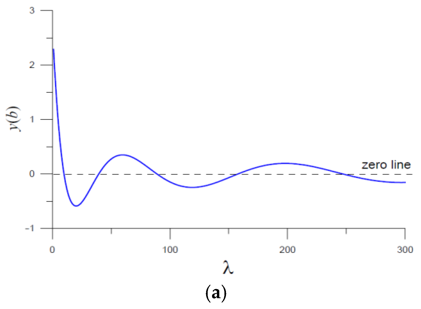
Then, we could apply the BSFM in Section 7.2 to solve this problem with $e_0=g_0=1,$ $B_0=1$, $s_{20}=1$, $C_1=C_2=1$, and $N=500$. Figure 5a shows a plot of the eigenvalue curve of $y^{\prime }\left(b\right)$ versus $\lambda$ in an interval [1, 1000] as a solid line, from which we can see that there were 10 zero points that corresponded to the first 10 eigenvalues ${\lambda }_k={\left(k+1\right)}^2{\pi }^2$, $k=0, 1,2,\dots , 9$.

By using the FTT and the FTIM, we compared the calculated eigenvalues to the exact ones for $k=0, 1,\dots , 4$ in

Table 5. Comparing the eigenvalues for Example 5 with the present BSFM using B₀ = 1 to the exact ones.

k	Exact	Example 5 (FTT)	Example 5 (FTIM)
0	9.86960440109	9.8696044010	9.86960440111
1	39.4784176044	39.4784176045	39.4784176054
2	88.8264396098	88.8264396099	88.8264396218
3	157.91367041743	157.91367041750	157.91367048410
4	246.7401100272	246.7401100273	246.7401102801

. It can be seen that the numerical errors were minimal—on the order of ${10}^{-11}$ to ${10}^{-10}$ when using the FTT and ${10}^{-11}$ to ${10}^{-7}$ when using the FTIM.

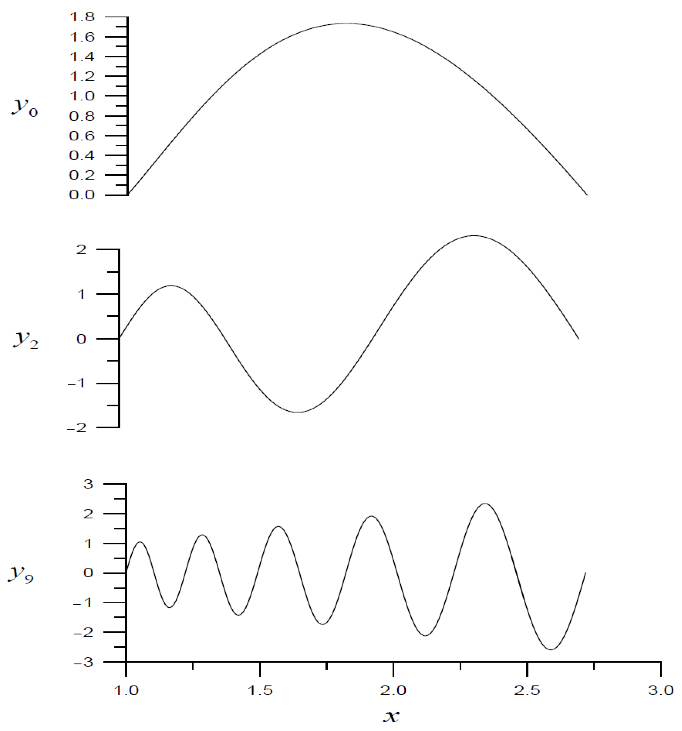
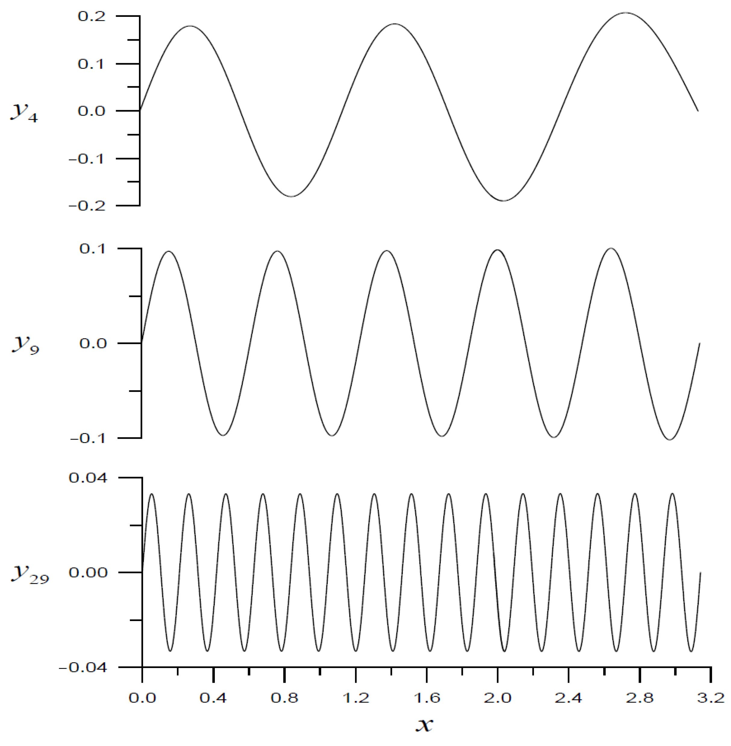
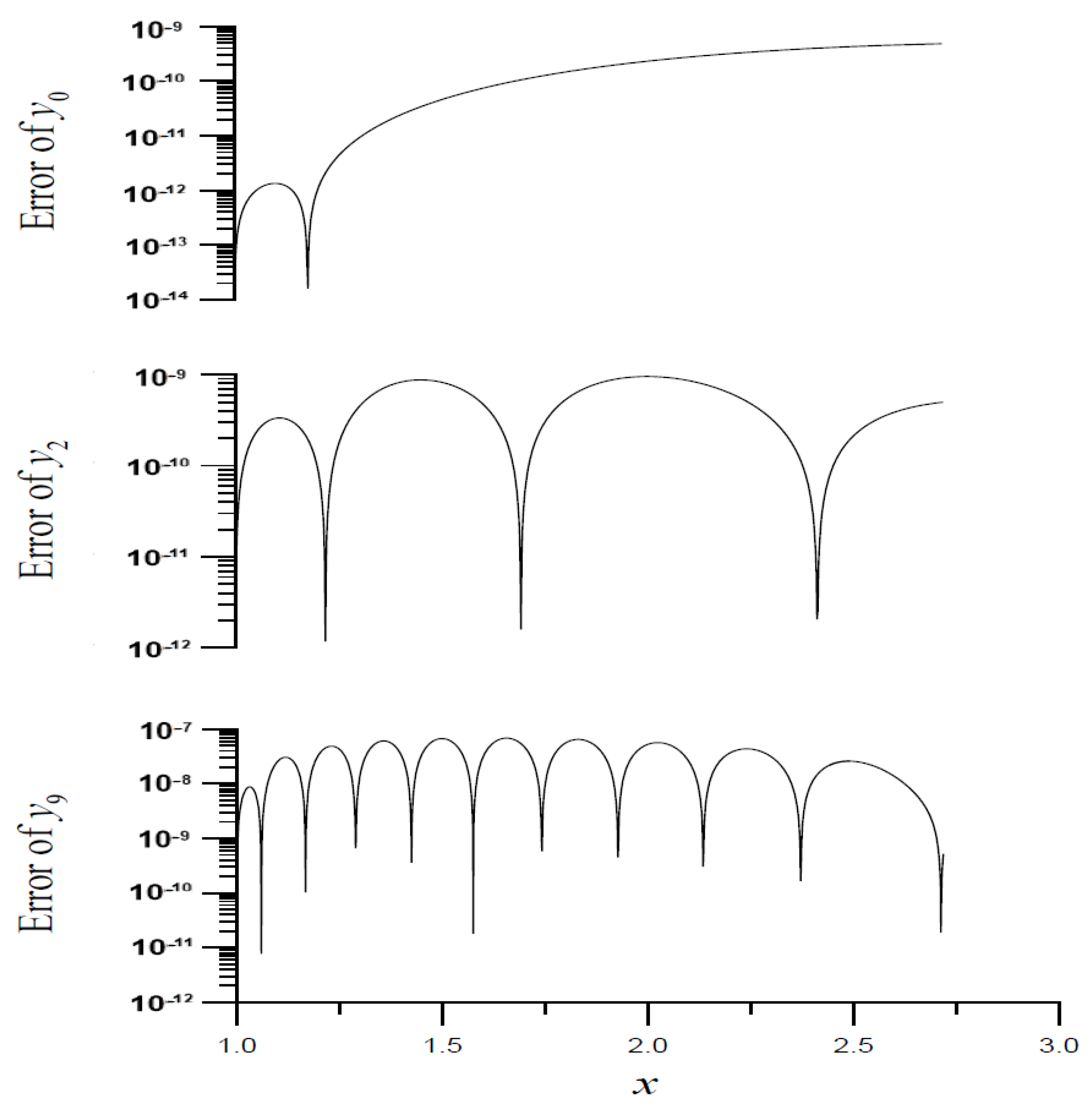
By tuning to finer intervals when using the FTT and applying the BSFM with $B_0=1$ or $B_0=2$, $s_{20}=1$, $C_1=C_2=1$, $N=1000$, and $M=101$, we could sequentially obtain the required eigenvalues; the calculated eigenfunctions for $k=0, 1, 5$ are shown in Figure 5b as solid lines. It can be seen that the numerical errors were minimal (on the order of ${10}^{-11}$ to ${10}^{-8}$ to satisfy the right boundary condition $u^{\prime }\left(x\right)+u\left(1\right)e_0/\left(1+e_0\right)=0,$ where we took $e_0=1$.

8.2. Example 6

At this moment, we solved the general SLP (1) and (2) by using Theorem 2 and the BSFM in Section 7.2. To test the accuracy, we considered:

$$-u^{″}\left(x\right)=\lambda u\left(x\right), x\in \left[0,1\right],$$

(103)

$$u\left(0\right)+{\mu }_1{u}^{\prime }\left(0\right)=0, u\left(1\right)+{\mu }_2{u}^{\prime }\left(1\right)=0,$$

(104)

where ${\lambda }_k,$ $k=0, 1, 2,\dots$ were solved using ${\mu }_1{\mu }_2{\lambda }^2\sin \lambda +\left({\mu }_2-{\mu }_1\right)\lambda \cos \lambda +\sin \lambda =0$; while the eigenfunctions were given by $u_k={\mu }_1{\lambda }_k\cos \left({\lambda }_{k}x\right)-\sin \left({\lambda }_{k}x\right)$.

For Example 5, we showed that using the FTT was more accurate than using the FTIM. We used the FTT to adjust the eigenvalues for the following examples. We applied the BSFM in Section 7.2 to solve this problem with ${\mu }_1=1$ or ${\mu }_2=-2$, $s_{20}=1$, $C_1=C_2=1$, $N=1000$, and $M=101$. By tuning to finer intervals using the FTT, we compared the calculated eigenvalues to the exact ones for $k=0, 2, 4$ in

Table 6. Comparing the eigenvalues for Example 6 with the present BSFM to the exact ones and showing the errors.

k	Exact	Present	Error
0	4.71336248921	4.71336248930	$8.87\times {10}^{-11}$
2	14.14008746763	14.14008746760	$3.41\times {10}^{-11}$
4	23.56681244606	23.56681244630	$2.43\times {10}^{-10}$

. It can be seen that the numerical errors were very small, on the order of ${10}^{-11}$ to ${10}^{-10}$.

8.3. Example 7

We considered Example 5 again; however, we used a different right boundary condition:

$$-u^{″}\left(x\right)+\frac{2}{{\left(x+1\right)}^2}u\left(x\right)=\lambda u\left(x\right), x\in \left[0,1\right],$$

(105)

$$u\left(0\right)+{\mu }_1{u}^{\prime }\left(0\right)=0, u\left(1\right)+2u^{\prime }\left(1\right)=0.$$

(106)

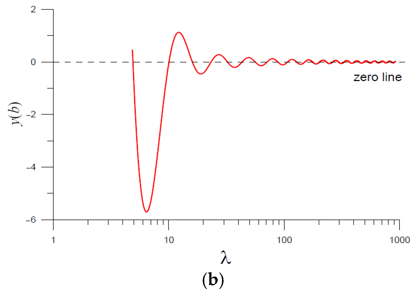
We employed Theorem 2 and applied the BSFM in Section 7.2 to solve this problem with $B_0=1$, $s_{20}=1$, $C_1=C_2=1$, $N=500$, and $M=2001$. Figure 5a shows a plot of the eigenvalue curve of $y^{\prime }\left(b\right)$ versus $\lambda$ by the dashed line in an interval $\left[1, 1000\right]$, from which we can see that there were 10 zero points that were close to the first 10 eigenvalues of Example 5. However, there were a few differences as shown in Table 5. The numerical errors of the eigenvalues were adjusted to be less than ${10}^{-6}$.

By tuning to finer intervals using the FTT and applying the BSFM in Section 7.2 with $B_0=1$, $C_1=C_2=1$, $\epsilon ={10}^{-8}$, and $N=1000$, we could sequentially solve for the required eigenvalues; the calculated eigenfunctions for $k=1, 3, 5$ are shown by the dashed lines in Figure 5b. The right boundary condition $u\left(1\right)-2u^{\prime }\left(1\right)=0$ could be satisfied very well, as shown in

Table 7. The eigenvalues for Example 7 with the present BSFM using B₀ = 1 and the right-boundary errors.

k	Eigenvalue	Right-Boundary Error
0	8.16809482500	$2.09\times {10}^{-11}$
1	37.9976982069	$1.73\times {10}^{-11}$
2	87.3754317150	$1.47\times {10}^{-11}$
3	156.472399123	$2.65\times {10}^{-11}$
4	245.303242649	$9.46\times {10}^{-12}$

.

8.4. Example 8

Now, we solved the general SLP (1) and (2) by using Theorem 3 and the BSFM in Section 5. We tested the following problem given in Example 5:

$$-u^{″}\left(x\right)+\frac{2}{{\left(x+g_0\right)}^2}u\left(x\right)=\lambda u\left(x\right), x\in \left[0,1\right],$$

(107)

$$u\left(0\right)+{\mu }_1{u}^{\prime }\left(0\right)=0, u\left(1\right)+{\mu }_2{u}^{\prime }\left(1\right)=0,$$

(108)

where ${\mu }_1=g_0$ and ${\mu }_2=1+g_0.$ This problem had the eigenvalues ${\lambda }_k={\left(k+1\right)}^2{\pi }^2$, $k=0, 1, 2,\dots$.

We applied the present BSFM based on Theorem 3 to solve this problem with $g_0=1$, $A_0=1$, $C_1=C_2=1$, $N=1000$, and $M=101$. By tuning to finer intervals using the FTT, the calculated eigenvalues were compared with the exact ones for ${\lambda }_k={\left(k+1\right)}^2{\pi }^2$, $k=0, 1, 2,\dots , 4$ in

Table 8. Comparing the eigenvalues for Example 8 with the present BSFM to the exact ones.

k	Exact	Present	Relative Error
0	${\pi }^2$	9.869604401	$3.173\times {10}^{-11}$
1	$4{\pi }^2$	39.47841762	$4.4096\times {10}^{-10}$
2	$9{\pi }^2$	88.82643980	$2.163\times {10}^{-9}$
3	$16{\pi }^2$	157.9136704	$1.267\times {10}^{-11}$
4	$25{\pi }^2$	246.74011002	$1.377\times {10}^{-13}$

. As shown in the table, the numerical errors were on the order of ${10}^{-13}$ to ${10}^{-9}$.

Remark 3. 

The Liouville transformation [26]:

$$v\left(t\right)=g\left(x\right)u\left(x\right), g\left(x\right)={\left[\omega \left(x\right)p\left(x\right)\right]}^{1/4},$$

(109)

$$t=\frac{1}{c}{\int }_a^x{\left(\frac{r\left(\tau \right)}{p\left(\tau \right)}\right)}^{1/2}d\tau , c={\int }_a^b{\left(\frac{r\left(\tau \right)}{p\left(\tau \right)}\right)}^{1/2}d\tau ,$$

(110)

can transform Equations (1) and (2) to the following canonical form:

$$-\ddot{v}\left(t\right)+Q\left(t\right)v\left(t\right)=\mu v\left(t\right), t\in \left[0,1\right],$$

(111)

$$h_{\ast }v\left(0\right)-\dot{v}\left(0\right)=0, H_{\ast }v\left(1\right)+\dot{v}\left(1\right)=0,$$

(112)

where:

$$Q\left(t\right)=c^2\frac{q\left(x\right)g\left(x\right)-{\left[p\left(x\right)g^{\prime }\left(x\right)\right]}^{\prime }}{\omega \left(x\right)g\left(x\right)}, \mu =c^2\lambda$$

(113)

$$h_{\ast }=cg\left(a\right)\left[hg\left(a\right)-p\left(a\right)g^{\prime }\left(a\right)\right], H_{\ast }=cg\left(b\right)\left[Hg\left(b\right)-p\left(b\right)g^{\prime }\left(b\right)\right].$$

(114)

The original SLP became a new SLP in the unit interval with the same eigenvalues multiplied by a constant factor $c^2$ and only the potential function $Q\left(t\right)$ was required.

Upon comparing the transform in Equation (109) to that in Equation (14), we could observe the similarity. However, $F\left(x\right)$ was an explicit quadratic or cubic function of $x$; all the coefficient functions were given explicitly in Equation (19). Moreover, the boundary conditions were more accessible to treat than Equation (112). One major drawback of Equation (111) was that the coefficient function $Q\left(t\right)$ was an implicit function of $t$, which could be known only after inverting the relation in Equation (110) to obtain the function $x=x\left(t\right)$ and then inserting it into Equation (113).

Both the transformations in Equations (14) and (109) were congruent, which maintained the linearity in the eigenvalue $\lambda$ or $\mu$. On the other hand, the transform (25) in Theorem 3 was not a congruent one, where the coefficient function $D\left(x,\lambda \right)$ is a linear function of $\lambda$ and $Q\left(x,\lambda \right)$ is a nonlinear function of $\lambda$. Nevertheless, from the aspect of the numerical method, the Dirichlet boundary conditions in Equation (24) were more uncomplicated and were easier to treat than the boundary conditions (20) and (112).

The SLP is very important in partial differential equations, vibrations in continuum mechanics, and heat conduction problems. We applied the Sturm–Liouville theory to solve the longitudinal wave motion problem when the Young’s modulus $E$ was fixed with the cross section area $A\left(x\right)=1+x$ of a tapered rod, a constant density $\rho$ of mass, and the axial displacement $y\left(x,t\right)$:

$$\frac{1}{A\left(x\right)}\frac{\partial }{\partial x}\left(EA\left(x\right)\frac{\partial y\left(x,t\right)}{\partial x}\right)=\rho \frac{{\partial }^{2}y\left(x,t\right)}{\partial t^2}.$$

(115)

Let $y\left(x,t\right)={\mathrm{e}}^{i\omega t}u\left(x\right)$ with $\omega$ as a natural vibration frequency; Equation (116) then reduces to Equation (4) with:

$$p\left(x\right)=EA\left(x\right), q\left(x\right)=0, \omega \left(x\right)=\rho A\left(x\right), \lambda ={\omega }^2.$$

(116)

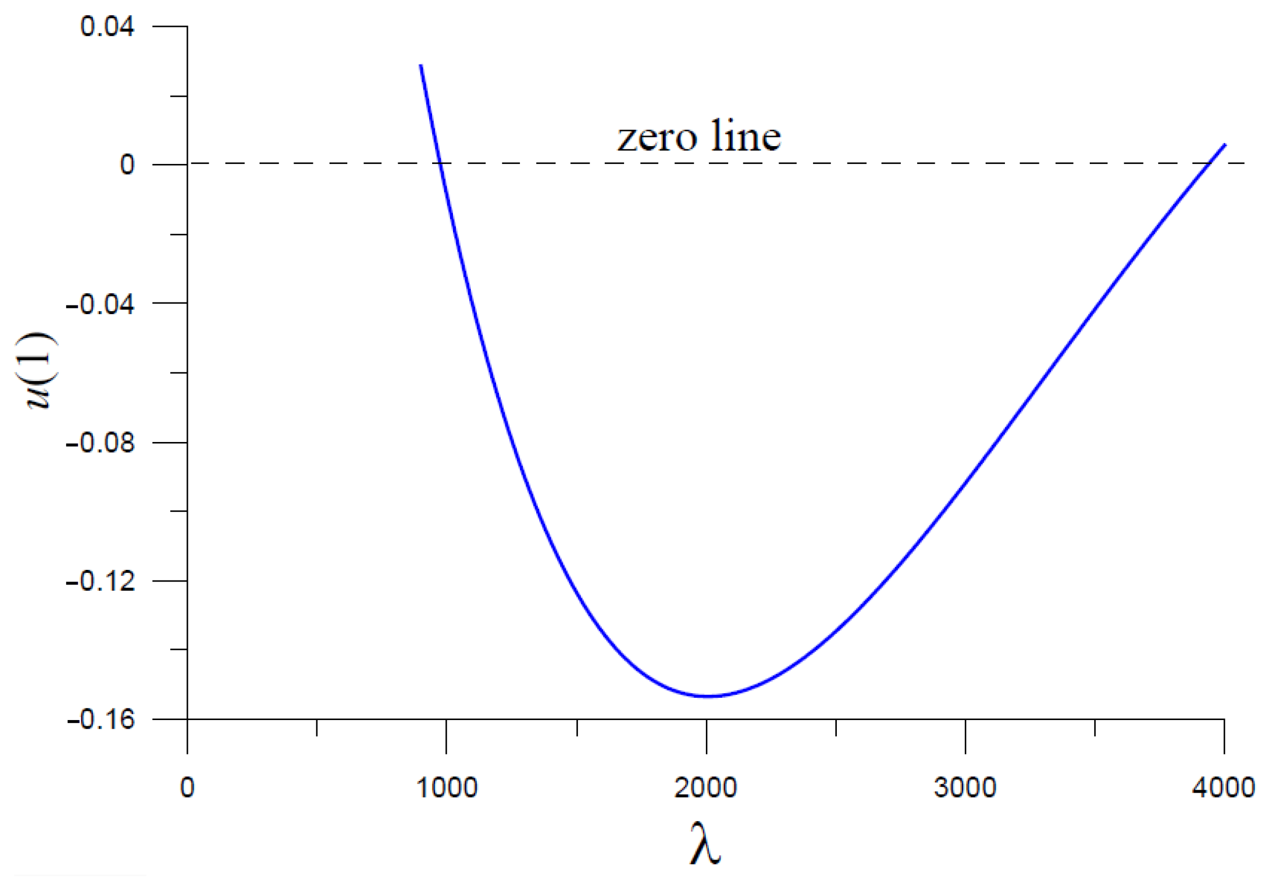
We fixed the length of the rod be a unit and took $E/\rho$ = 100.

In the design of engineering structures, knowing first few frequencies $\omega$ is of utmost importance. Figure 6 shows a plot of $u\left(1\right)$ versus $\lambda$ in a range of $\lambda \in \left[0,4000\right]$, where two intersecting points appeared. Then, by tuning to finer intervals, we could obtain ${\mathsf{\lambda }}_0=975.3318666643578$ and ${\mathsf{\lambda }}_1=3935.600370373466$.

9. Conclusions

For the SLPs with the Sturm–Liouville boundary conditions, we derived two novel transformations that could transform them into two canonical forms with either the Dirichlet boundary conditions or the Neumann boundary conditions. These two canonical forms appeared in the literature at the same time. Numerically, these two simpler forms were more easily treated than the original Sturm–Liouville-type boundary conditions. The major novelty of the paper was that we employed the shape function to transform the Sturm–Liouville boundary value problem to the corresponding initial value problem for the new variable with terminal values that could be determined explicitly by using the Neumann-type normalization condition for the Dirichlet canonical form and the Dirichlet-type normalization condition for the Neumann canonical form. Based on these novel ingredients in the BSFM, we could solve the Sturm–Liouville problems easily and directly. In the BSFM, the only unknown constant was the eigenvalue, which was determined by solving the derived algebraic equation with a finer tuning technique or by using the fictitious time integration method. Eight numerical examples confirmed the high performance of the new BSFM algorithm based on methods with high accuracy for the obtained eigenvalues and eigenfunctions. As compared to the conventional shooting method, we did not need to guess the missing initial value. The advantages of the presented two novel transformations were explored when we compared them to the Liouville transform. Future works can focus on extending the BSFM to solve generalized Sturm–Liouville problems and periodic Sturm–Liouville problems in terms of nonlinear problems.