Role of Glucose Risk Factors on Human Breast Cancer: A Nonlinear Dynamical Model Evaluation

Abstract

Understanding of the glucose risk factors-mediated mechanism in human breast cancer remains challenging. In this perception, for the first time, we proposed a complex nonlinear dynamical model that may provide a basic insight into the mechanism of breast cancer for the patient with existing glucose risk factors. The impact of glucose risk factors on the cancer cells’ population is evaluated using the formulated analytical model. The dynamical features of the cancer cells are described by a system of ordinary differential equations. Furthermore, the Routh–Hurwitz stability criterion is used to analyze the dynamical equilibrium of the cells’ population. The occurrence of zero bifurcation as well as two and three of the Jacobian matrix are obtained based on the sums of principal minors of order one. The glucose risk factors are exploited as the bifurcation parameters (acted as necessary and sufficient conditions) to detect the Hopf bifurcation. The presence of excess glucose in the body is found to affect negatively the breast cancer cells’ dynamics, stimulating chaos in the normal and tumor cells and thus drastically deteriorating the efficiency of the human immune system. The theoretical results are validated using the numerical simulations. It is concluded that the present findings may be beneficial for the future breast cancer therapeutic drug delivery and cure.

1. Introduction

Human cancers are one of the most deadly diseases with life-threatening attributes, yet they remain incurable despite the advancement of modern medicines and surgical procedures. In general, there are many types of cancers such as blood, skin, colon, lung, breast, etc. to cite a few. Amongst all these, breast cancer is more prevalent in women than men, thereby causing several million deaths annually worldwide [1,2,3]. An estimate by the global cancer statistics of 2020 revealed that breast cancer in women is becoming very common with approximately 2.3 million new cases every year (11.7%), thus rapidly surpassing lung cancer (11.4%), colorectal cancer (10.0%), prostate cancer (7.3%), and stomach cancer (5.6%) [4]. Numerous studies have continually been conducted to determine the complex mechanism of cancer cells dynamics and growth processes, providing new knowledge to improve the cancer treatment, drug delivery, and therapeutic strategies. In spite of many dedicated efforts, various significant factors that are responsible for the breast cancer development in the tissues such as estrogen excess and nutrients are far from being understood. In addition, the glucose risk factors-mediated processes in human breast cancer that impart further impetus need to be explored.

Over the decades, diverse mathematical models have been introduced to examine the dynamical behavior of the cancer cells in the presence of varied factors. Roberto et al. [5] proposed a mathematical model to evaluate the effects of obesity as a risk factor on the tumor growth and immune response. In addition, several models were presented to show that the stored fat in an obese human body contributes considerably to the tumor growth, thus increasing the risk factors toward survival [6]. The impact of an unhealthy diet as one of the risk factors for cancer was evaluated using an analytical model [7]. The results obtained from the model simulation displayed that the immune cells’ boost up through the intervention of vitamins can delay the mechanisms of the tumor cells’ growth and division. Admon and Maan [8] constructed a mathematical model to determine the effect of immune response and drugs on the growth mechanisms of tumor cells. The results demonstrated that the combination of immune and drug can provide a better way to kill the tumor cells. Mufudza et al. [9] assessed the impact of estrogen on the dynamics of normal, breast cancer, and immune cells using a system of ordinary differential equations (ODEs). It was concluded that extra estrogen can increase the degree of tumor formation and inhibit the immunity development. Oke et al. [10] extended the model proposed by Mufudza et al. [9] in the context of chemotherapy treatment and the ketogenic diet. A set of ODEs was applied to examine the breast cancer cells’ dynamics in the presence of chemotherapy medicine and ketogenic diet. It was affirmed that an increase in the level of estrogen can appreciably affect the dynamical stability of the cells’, accelerating the growth of tumor. In addition, the presence of the ketogenic diet during treatments was shown to reduce the number of cancer cells to zero when the reproductive number of a certain threshold was less than one. The level of the immune system, anti-cancer treatment effectiveness, and ketogenic diet dose rates could contribute to reducing the breast cancer risk, while an increase in the estrogen level could improve the formation rate of the tumor. Meanwhile, many mathematical models used the bifurcation analysis to determine the behavior of cells under a specific parameter. The chaos of cells was shown to occur when the value of a specific parameter is changed over time.

More recently, fractional differential equations have been used in a cancer growth model to determine the tumor-immune dynamics [11]. The chaotic behaviors of the proposed cancer model for both commensurate and incommensurate cases have been understood in terms of the bifurcation diagram, Lyapunov exponent, and phase plot. It was concluded that various chaotic behaviors can emerge when the derivative’s order surpasses the threshold limit. Consequently, it becomes impossible to predict the number of healthy host, tumor, and effector cells [11]. Another investigation [12] was made to examine the tumor cells’ characteristics when the immune response is absent, wherein the tumor, normal, and fat cells were inspected using bifurcation in order to identify the chaotic regime. The findings exhibited the occurrence of codimention-1 bifurcation of the system and the complete absence of any periodic solutions. This in turn suggested an eventual deterioration of the condition and non-existence of Hopf bifurcation.

It is established that cancer cells display the aerobic glycolysis process, implying that such cells obtain most of their energy from the glycolysis, wherein glucose is transformed to lactate for energy after its fermentation even during the accessibility of oxygen, which is a phenomenon called the Warburg effect [13]. In addition, resembling other types of cancer cells, the breast carcinoma cell lines display dependency on glucose, deriving most of their energy as adenosine triphosphate (ATP) from high-throughput glycolysis [14]. Numerous studies confirmed that cancer cells feed heavily on glucose; thus, they are included in the model to determine its effect on the breast cancer cells. Chen et al. [15] examined the role of glucose deprivation during the breast cancer cells’ death. Wardi et al. [16] showed that excessive glucose intake can increase and proliferate the cancer cells development, while glucose restriction can reduce and inhibit the cancer cells’ growth.

Santos and Hussain [2] evaluated the influence of glucose on the breast cancer cells. It was asserted that a higher glucose level can enhance the breast cancer cells’ aggressiveness, wherein glucose facilitates its rapid growth and spread. Furthermore, the results showed that a higher glucose level can speed up the cells’ migration, proliferation, and growth. Kretowski et al. [17] claimed that since glucose is the major energy resource for the tumor cells’ development, an elevated amount of intracellular glucose enables the cancer cells proliferation due to their strong glucose-dependent metabolism. Barbosa and Martel [18] argued that cancer cells require a higher amount of glucose even when oxygen is accessible, displaying more sensitivity to the glucose deprivation-mediated death compared to the normal cells. Hence, the inhibitors for the glucose uptake must be regarded as a kind of breast cancer cure. It was acknowledged that [19] a high level of glucose can strongly support the cell proliferation. Furthermore, the cells showed a greater invasion and proliferation capacity in a high glucose-containing medium than the one in a normal glucose medium. It clearly verified the effect of high glucose contents in promoting the cancer cells’ spreading in the body.

A high quantity of glucose can lead to an impaired function of the immune system and pathological conditions. Nevertheless, an appropriate quantity of glucose is essential for the immune system. An elevated amount of glucose can cause the production of extreme pro-inflammatory cytokines. Consequently, the infiltration of the high quantity of glucose into the immune cells can adversely affect the immune system and associated signal transfer pathways, leading to the generation of pro-inflammatory cytokines. This in turn leads to an impaired function of the immune system, triggering pathological situations [20]. To sum up, the majority of the previous studies confirmed that high glucose intake can enhance the growth and proliferation of the breast cancer cells, thus providing a fertile environment for the rapid development of breast cancer. Conversely, only a few studies have been conducted to determine the effect of glucose on the human immune system. It was demonstrated a high or low glucose rate in the body can negatively influence the immune cells [21]. It is needless to mention that although several studies have qualitatively assessed the role of glucose (as main energy source) on the breast cancer cells’ dynamics [2,13,16,17,18,19,20,21,22], a comprehensive mathematical model that quantifies the impact of glucose on the complex dynamical mechanisms of breast cancer cells is missing. It is established that glucose is the main energy source of the cancer cells for their growth and proliferation [2]. Thus, the cancer cells’ spread, promotion, and the differentiation and conversion into quiescent cells can be reduced with the lowering of glucose intake [16]. In order to achieve a quantitative estimate concerning the excess glucose intake by the breast cancer cells and their negative impact on the normal, cancer, and immune cells in further deteriorating the patient immune system, a systematic study is essential. The symmetric and antisymmetric concepts between a realistic biological behavior and the dynamics system of cells play an essential role in reducing cancer risks. Considering the immense fundamental significance of understanding the adverse impact of the glucose risk factors on human breast cancer, we developed an analytical model to determine the mechanisms of breast cancer cells dynamics in the presence of glucose. In addition, the influence of glucose as nutrients on the cancer cells’ growth, proliferation, invasion capacity into healthy tissues and thereafter rapid spreading in the patient body is emphasized.

This article is structured as follows: Section 2 formulates the proposed nonlinear dynamical model for breast cancer. Section 3 provides the local stability analyses and criteria for the equilibrium. Section 4 analyzes the existence conditions for the zero and Hopf bifurcation. Section 5 presents the results obtained from the numerical simulation of the model and validates it. Section 6 briefly discusses the salient features of the results and concludes the study with further outlook.

2. Formulation of Nonlinear Dynamical Model for Breast Cancer

In this work, we modified the earlier model of breast cancer with glucose risk factors introduced in [9]. The proposed three-dimensional (3D) deterministic model incorporates the host (normal), tumor, and immune cells of the breast cancer patient in the presence of excess glucose-stimulated risk factors. The model is formulated based on the following assumptions:

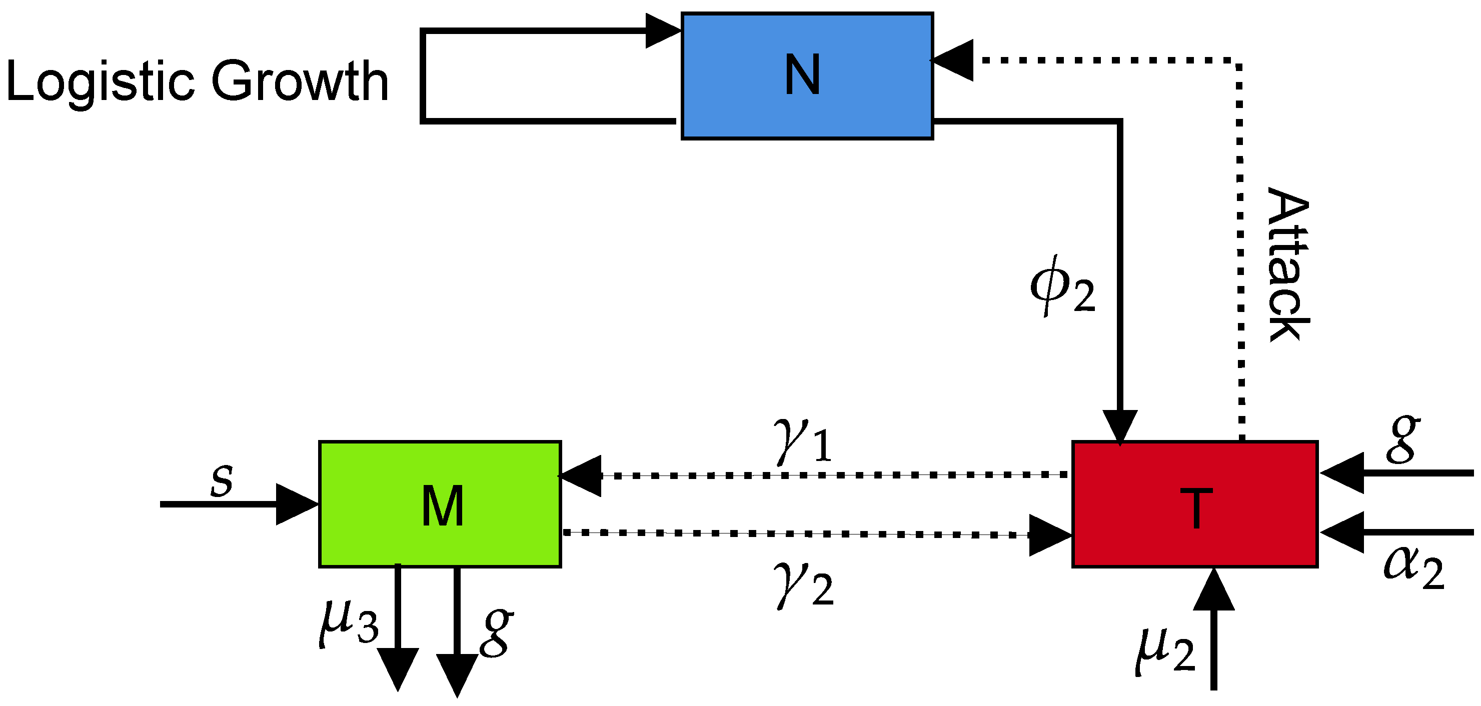
• The category of host (normal) epithelial cells ($N\left(t\right)$) at any time (t) is composed of the breast tissues. The life cycle of $N\left(t\right)$ follows the logistic growth $N\left(t\right)\left[{\alpha }_1-{\mu }_{1}N\left(t\right)\right]$, where ${\alpha }_1$ and ${\mu }_1$ are the corresponding growth and death rate of the normal breast cells, respectively.
• The category of tumor cells ($T\left(t\right)$) and their concentration is entirely different from the normal cells. The cell divisions in this class occur rapidly in an uncontrolled manner. The natural death of tumor cells has no biological meaning; however, their growth can be inhibited due to some factors such as immune suppression. The growth of tumor cells is described by $T\left(t\right)\left[{\alpha }_2-{\mu }_{2}T\left(t\right)\right]$, wherein ${\alpha }_2$ and ${\mu }_2$ are the corresponding growth and inhibition rate of the breast tumor cells, respectively.
• The reasons for the appearance of the tumor cells in tissues are usually unknown. However, many studies argued that the occurrence of tumors may be due to various internal and external factors [23]. The factors such as cell damage, some hormones, immune cell weakness and others are classified as internal types. Conversely, the external factors include lifestyle, sleeping habits, stress, and exercise activity. These factors may transform a normal cell into a tumor cell. It is further assumed that the normal cells compete strongly with the tumor cells to gain space and energy resources in a tiny volume, justifying our acceptance of the competition model proposed by Mufudza et al. [9]. In essence, the interaction between tumor and normal cells can be represented as ${\varphi }_{1}NT$, where ${\varphi }_1$ is the competition-induced death rate of the normal cells.
• Following the recommendation of [7], wherein due to the competition between tumor and normal cells, the former ones (tumor) grow rapidly at the expense of later ones (normal), one can write ${\varphi }_{2}N\left(t\right)T\left(t\right)$. Herein, ${\varphi }_2$ denotes the competition-induced growth rate of the tumor cells.
• Numerous studies [2,13,16,17,18,19,20,21,22] indicated that new cancer cells are formed with the increase of glucose contents in the patient body. New tumor cells are denoted by $gT\left(t\right)$, where g represents the rate of glucose excess.
• The human immune system is mainly responsible for the protection of the body from the growth of tumor cells, which are generated and die on daily basis [24,25]. The immune cells ($M\left(t\right)$) in the absence of a tumor can be written as $\left[s-{\mu }_{3}M\left(t\right)\right]$, where s and ${\mu }_3$ are the corresponding growth and natural death rates of the immune cells.
• The activity status of the tumors can boost the human immune system. A positive nonlinear growth term of the form $\frac{\rho M\left(t\right)T\left(t\right)}{\omega +T\left(t\right)}$, where $\rho$ and $\omega$ are the respective immune response and threshold rates (inversely proportional to the steepness of the immune response curve) related to the immune cells, can be used to represent such activity status.
• Both cells (tumor and immune cells) can fight with others, but immune cells have the capacity to fight with the foreign cells only. Hence, the tumor and immune cells might be reduced during the interaction process. We denote the competition via ${\gamma }_{1}M\left(t\right)T\left(t\right)$ and ${\gamma }_{2}M\left(t\right)T\left(t\right)$, wherein ${\gamma }_1$ is the reduction of the tumor cells by the immune cells action and ${\gamma }_2$ is the decrease of the immune cells by the tumor cells. It is worth noting that the ability of the immune cells to invite the fringe can be affected by various factors such as excess blood glucose rate, impacting the immune system efficacy [20,21] written as $gM\left(t\right)$.

Based on these postulates, the complete model can be casted as:

$$\begin{array}{ccc}\hfill \frac{dN}{dt}& =& N\left({\alpha }_1-{\mu }_{1}N\right)-{\varphi }_{1}NT,\hfill \\ \hfill \frac{dT}{dt}& =& T\left({\alpha }_2-{\mu }_{2}T\right)+gT-{\gamma }_{1}MT+{\varphi }_{2}NT,\hfill \\ \hfill \frac{dM}{dt}& =& s+\frac{\rho MT}{\omega +T}-{\gamma }_{2}MT-{\mu }_{3}M-gM.\hfill \end{array}$$

(1)

All parameters in the model (1) are positive with the initial conditions

$$N\left(0\right)>0,T\left(0\right)\ge 0andM\left(0\right)>0.$$

Figure 1 shows the competition among the cells population in the proposed nonlinear dynamical model of breast cancer.

3. Model Analysis

3.1. Boundedness and Positive Invariance

We need to demonstrate that the model with the chosen parameter values is biologically plausible before we move on to the mathematical analysis by proving the boundness and positivity of solutions.

Since our model investigates cellular populations, therefore, all the variables and parameters of the model are non-negative. Based on the biological finding, the system will be studied in the following region: $\mathrm{\Psi }=\{(N,T,M)\in R_{+}^3\}$

Theorem 1.

The region $\mathrm{\Psi }\subset R_{+}^3$ of the dynamic system (1) is positively invariant, and non-negative solution exists for all time t.

Proof. 

Let $\mathrm{\Psi }={\mathrm{\Psi }}_c\subset R_{+}^3$ with $\mathrm{\Psi }=\{(N,T,M)\in R_{+}^3:N\le \frac{{\alpha }_1}{{\mu }_1},T\le \frac{{\alpha }_2+g}{{\mu }_2},M\le \frac{s}{{\mu }_3+g}\}$; then, the solutions of $N\left(t\right),T\left(t\right),M\left(t\right)$ in the dynamic system (1) are positive for any time t. From the first equation of system (1), it is obvious that

$$\frac{dN}{dt}\le {\alpha }_{1}N-{\mu }_1{N}^2$$

solving this equation with Bernouli method, we obtain

$$N\left(t\right)\le \frac{{\alpha }_1}{{\mu }_1+c{\alpha }_1{e}^{-{\alpha }_{1}t}}$$

(2)

and as $t\to \infty$

$$N\left(t\right)\le \frac{{\alpha }_1}{{\mu }_1}.$$

Now, for the second equation of system (1), we have

$$\frac{dT}{dt}\le {\alpha }_{2}T-{\mu }_2{T}^2+gT$$

using the Bernouli method to solve this equation, we obtain

$$T\le \frac{{\alpha }_2+g}{{\mu }_2+({\alpha }_2+g)c{e}^{-({\alpha }_2+g)t}}$$

then, the solution is given as

$$T\le \frac{{\alpha }_2+g}{{\mu }_2}, \mathrm{as} t\to \infty$$

The last equation of system (1) satisfies

$$\frac{dM}{dt}\le s-{\mu }_{3}M-gM$$

then the solution of this equation will give

$$M\le \frac{s}{{\mu }_3+g}+c{e}^{-({\mu }_3+g)t}$$

and as $t\to \infty$, we obtain the solution

$$M\le \frac{s}{{\mu }_3+g}$$

this completes the proof. □

3.2. Existence of Equilibrium Points

The equilibrium of the solutions of the model equations can be obtained by setting the left-hand side equal to zero:

$$\frac{dN}{dt}=\frac{dT}{dt}=\frac{dM}{dt}=0.$$

(3)

Solutions of System (1) yield four steady states with two dead equilibrium points, one tumor-free equilibrium point, and one coexisting equilibrium point. The following sections discusses the salient features of these states.

3.2.1. Tumor-Free Equilibrium $E_0$:

Herein, $E_0$ signifies that only the tumor cells’ population is vanished or enforced to extinct due to the competitive interactions among tumor, immune and normal cells. The value of $E_0$ can be obtained via:

$$E_0=\left(N^{\ast },T^{\ast },M^{\ast }\right)=\left(\frac{{\alpha }_1}{{\mu }_1},0,\frac{s}{g+{\mu }_3}\right).$$

(4)

Clearly, $E_0$ exists if and only if the parameters ${\alpha }_1,{\mu }_1,s,g$ and ${\mu }_3$ have real positive values, indicating that all the solutions around $E_0$ are feasible.

Biologically, this case is called the healthy case for the patient where the tumor disappears, while normal cells and immune cells remain. This point can be explained as follows: the glucose level is very low, which makes the tumor environment unprepared and thus facilitates the elimination of cancer cells by immune cells.

3.2.2. Type 1 Dead Equilibrium $E_1$

Herein, $E_1$ implies that in the entire cells’ population, only the normal cells died and tumor cells survived. The ability of a cancer cell to ‘escape malignancy’ and transformed back to a normal state might seem impossible. Thus, it is labeled as a “dead” case of equilibrium point. In fact, the recovery of the damaged normal cells is none, because they are forced to become extinct. This condition yields:

$$E_1=\left(N^{\ast },T^{\ast },M^{\ast }\right)=\left(0,\frac{1}{{\mu }_2}\left(g+{\alpha }_2-{\gamma }_1{M}^{\ast }\right),M^{\ast }\right),$$

(5)

with

$$M^{\ast }=\frac{{\gamma }_2\left[\omega {\mu }_2+2\left(g+{\alpha }_2\right)\right]+{\mu }_2\left(g+{\mu }_3-\rho \right)}{3{\gamma }_1{\gamma }_2}.$$

(6)

Obviously, $E_1$ exists if and only the parameters $g,\rho ,\omega ,{\alpha }_2,{\mu }_2,{\mu }_3,{\gamma }_1$ and ${\gamma }_2$ are positive and the following conditions are obeyed:

$$g>max\{\rho -{\mu }_3,\frac{{\mu }_2({\gamma }_2\omega +{\mu }_3-\rho )-{\gamma }_2{\alpha }_2}{{\gamma }_2-{\mu }_2}\}$$

(7)

Biologically, this point is classified as glucose risk such that the rate of glucose is greater than the rate of the immune response, which contributes to the growth of cancer cells at a much higher rate than normal cells. In this case, the tumor spreads, and the patient becomes in a critical condition, leading to either mastectomy or death. The mathematical result confirmed the biological results: if the glucose rate is higher than the immune response rate, the point will be in the feasible region of the system. The immune response appeared due to the high glucose rate, contributing to tumor growth. Hence, it confirms that high glucose negatively affects the immune system, as mentioned in [20,21].

3.2.3. Type 2 Dead Equilibrium ($E_2$):

In this case, $E_2$ exists if and only if both the tumor and normal cells’ population vanish. The values of $E_2$ can be estimated using:

$$E_2=\left(N^{\ast },T^{\ast },M^{\ast }\right)=\left(0,0,\frac{s}{g+{\mu }_3}\right).$$

(8)

Herein, $E_2$ is finite if and only if all parameters $s,g$ and ${\mu }_3$ have real positive values, indicating that all solutions in the proximity of $E_2$ are realistic. Although this is an interesting possibility, no tissues exist in reality because of the entire breast tissues removal by a mastectomy surgery or the patient’s death. In fact, $E_2$ makes no sense biologically and is not realistic because it is not acceptable that $N=T=0$ while $M\ne 0$, which means that immune cells exist. The task of immune cells is to protect the normal cells or fight diseases, but in the case of breast cancer, these cells are not active unless there are normal cells or a tumor. Therefore, the only possible explanation for this case is that either the breast was removed or the patient died.

3.2.4. Coexisting Equilibrium $E_3$:

$E_3$ signifies that all types of cells population survived in the competition, and their coexistence can mathematically be expressed as:

$$E_3=\left(N^{\ast },T^{\ast },M^{\ast }\right)=\left(\frac{1}{{\mu }_1}\left({\alpha }_1-{\varphi }_1{T}^{\ast }\right),T^{\ast },\frac{1}{{\gamma }_1{\gamma }_2{\mu }_1}\left({\gamma }_2{l}_2-k_1{T}^{\ast }\right)\right),$$

(9)

where $T^{\ast }$ can be represented by the real positive zeros of the system of cubic equations of the form:

$$k_1{\left(T^{{}^{\ast }}\right)}^3+k_2{\left(T^{{}^{\ast }}\right)}^2+k_3{T}^{\ast }+k_4=0,$$

(10)

$$\begin{array}{ccc}\hfill k_1& =& {\gamma }_2\left({\mu }_1{\mu }_2+{\varphi }_1{\varphi }_2\right)>0,\hfill \\ \hfill k_2& =& \frac{k_1}{{\gamma }_2}{l}_1-{\gamma }_2{l}_2,\hfill \\ \hfill k_3& =& \frac{\omega }{{\gamma }_2}{k}_1\left(g+{\mu }_3\right)-l_1{l}_2+s{\gamma }_1{\mu }_1,\hfill \\ \hfill k_4& =& -\omega \left[\left(g+{\mu }_3\right)l_2-s{\gamma }_1{\mu }_1\right],\hfill \end{array}$$

(11)

and

$$\begin{array}{ccc}\hfill l_1& =& \omega {\gamma }_2+g+{\mu }_3-\rho ,\hfill \\ \hfill l_2& =& {\mu }_1\left(g+{\alpha }_2\right)+{\alpha }_1{\varphi }_2.\hfill \end{array}$$

Substituting $T^{\ast }=\eta -\frac{k_2}{3k_1}$ into Equation (10), all equation numbers must be changed, and one obtains:

$${\eta }^3+U\eta +V=0,$$

(12)

where $U=\frac{k_3}{k_1}-\frac{1}{3}{\left(\frac{k_2}{k_1}\right)}^2$ and $V=\frac{k_4}{k_1}+\frac{2}{27}{\left(\frac{k_2}{k_1}\right)}^3-\frac{k_2{k}_3}{3k_1^2}.$

Next, let $3AB=-U$ and $A^3+B^3=-V;$ then, we obtain

$$A={\left(-\frac{V}{2}+\sqrt{D}\right)}^{1/3},$$

$$B={\left(-\frac{V}{2}-\sqrt{D}\right)}^{1/3},$$

where $D={\left(\frac{V}{2}\right)}^2+{\left(\frac{U}{3}\right)}^3.$

The solutions of Equation (12) take the form:

$$\begin{array}{ccc}\hfill {\eta }_1& =& A+B,\hfill \\ \hfill {\eta }_{2,3}& =& -\frac{1}{2}\left(A+B\right)\pm i\sqrt{3}\left(A-B\right),\hfill \end{array}$$

(13)

where $i^2=-1.$ The solution of Equation (12) depends on the sign of the discriminant D with the following possibilities [26]:

• For $D>0$, we achieve one real root and two imaginary roots.
• For $D<0$, one achieves three real roots.
• For $D=0$ and $U=V=0$, we obtain one simple real root with a multiplicity of three.
• For $D=0$ and ${\left(\frac{U}{3}\right)}^3=-{\left(\frac{V}{2}\right)}^2\ne 0$, one obtains thee real roots with single and double multiplicity.

Algebraic manipulations of Equations (9)–(13) indicate that $E_3$ can exist under the condition:

$$0<T^{\ast }<min\left\{\frac{{\alpha }_1}{{\varphi }_1},\frac{{\gamma }_2{l}_2}{k_1}\right\}.$$

(14)

The coexisting point represents the interaction stage among normal, cancer, and immune cells. All cells compete for survival in this stage. The immune cells are activated as a result of tumor appearance.

3.3. Local Stability of Equilibrium

It is important to perform the local stability analysis of the equilibrium points such as $E_0$, $E_1,E_2$ and $E_3$ to obtain a basic insight into the breast cancer cells’ dynamics. The following Jacobian matrix $J\left(E_{\ast }\right)$ was computed to determine the local stability of the equilibrium:

$$J\left(E_{\ast }\right)=\left[\begin{array}{ccc}{\alpha }_1-2{\mu }_1{N}^{\ast }-{\varphi }_1{T}^{\ast }& -{\varphi }_1{N}^{\ast }& 0\\ {\varphi }_2{T}^{\ast }& -{\gamma }_1{M}^{\ast }+{\varphi }_2{N}^{\ast }-2{\mu }_2{T}^{\ast }+g+{\alpha }_2& -{\gamma }_1{T}^{\ast }\\ 0& M^{\ast }\left(\frac{\rho \omega }{{\left(\omega +T^{\ast }\right)}^2}-{\gamma }_2\right)& T^{\ast }\left(\frac{\rho }{\omega +T^{\ast }}-{\gamma }_2\right)-\left({\mu }_3+g\right)\end{array}\right].$$

(15)

Theorem 2.

The tumor-free equilibrium point $E_0$ is characterized by:

• Asymptotically stable (sink) if $g<g_0.$
• Unstable (saddle) if $g>g_0.$
• Nonhyperbolic if $g=g_0$.

where $g_0$ is given by:

$$g_0=\frac{\sqrt{\Delta }-({\alpha }_1{\varphi }_2+{\alpha }_2{\mu }_1+{\mu }_1{\mu }_3)}{2{\mu }_1},$$

(16)

and

$$\begin{array}{ccc}\hfill \Delta & =& {\left({\alpha }_1{\varphi }_2+{\alpha }_2{\mu }_1+{\mu }_1{\mu }_3\right)}^2-4{\mu }_1\left({\alpha }_1{\mu }_3{\varphi }_2+{\alpha }_2{\mu }_1{\mu }_3-s{\gamma }_1{\mu }_1\right)>0,\hfill \\ \hfill s& >& s_0=\frac{{\mu }_3}{{\gamma }_1{\mu }_1}\left({\alpha }_1{\varphi }_2+{\alpha }_2{\mu }_1\right).\hfill \end{array}$$

Proof. 

Substituting the equilibrium point $E_0$ (4) into (15), one obtains the following variational matrix:

$$J\left(E_0\right)=\left[\begin{array}{ccc}-{\alpha }_1& \frac{-{\alpha }_1{\varphi }_1}{{\mu }_1}& 0\\ 0& -\frac{{\gamma }_{1}s}{{\mu }_3+g}+\frac{{\varphi }_2{\alpha }_1}{{\mu }_1}+g+{\alpha }_2& 0\\ 0& \frac{s\left(\rho -\omega {\gamma }_2\right)}{\omega \left({\mu }_3+g\right)}& -\left({\mu }_3+g\right)\end{array}\right].$$

(17)

The characteristic equations of $J\left(E_0\right)$ yield the eigenvalues:

$$\begin{array}{ccc}\hfill {\lambda }_1& =& \frac{{\mu }_1{g}^2+\left({\alpha }_1{\varphi }_2+{\alpha }_2{\mu }_1+{\mu }_1{\mu }_3\right)g+\left({\alpha }_1{\mu }_3{\varphi }_2+{\alpha }_2{\mu }_1{\mu }_3-s{\gamma }_1{\mu }_1\right)}{\left({\mu }_3+g\right){\mu }_1},\hfill \\ \hfill {\lambda }_2& =& -\left({\mu }_3+g\right),\hfill \\ \hfill {\lambda }_3& =& -{\alpha }_1.\hfill \end{array}$$

It is clear that ${\lambda }_2$ and ${\lambda }_3$ are always negative. The solution of ${\lambda }_1=0$ in terms of g yields one positive zero when $g=g_0$ such that $s>s_0=\frac{{\mu }_3}{{\gamma }_1{\mu }_1}\left({\alpha }_1{\varphi }_2+{\alpha }_2{\mu }_1\right)$. One can deduce that $\left({\lambda }_1<0,{\lambda }_1>0\right)$ for $\left(g<g_0,g>g_0\right)$. In addition, if $g<g_0$, then all eigenvalues of matrix (17) are negative, indicating $E_0$ as a local asymptotic stable point. Conversely, for $g>g_0$, i.e., ${\lambda }_1>0$, $E_0$ is a saddle point. For $g=g_0,$ then $J\left(E_0\right)$ has only one zero eigenvalue, making $E_0$ a nonhyperbolic point. □

Biologically, cancer cells depend on their ability to reproduce and absorb glucose, which means that if the rate of glucose is lower than $g_0$, it will contribute significantly to the inhibition of cancer cells and reduce their strength and ability to reproduce and spread. This leads to the stability of the patient’s health. Many studies focused on this characteristic of cancer cells. Therefore, they recommended some methods to reduce the amount of glucose entering the body, such as a low-carb or ketogenic diet [10] and avoiding unhealthy ones. In addition, recent studies are now focusing on studying the effect of glucose uptake inhibitor drugs or inhibiting glucose transporters as an anti-cancer treatment to reduce tumor cancer cell proliferation [18,27,28,29].

Theorem 3.

The type 1 dead equilibrium point ($E_1$) is unstable.

Proof. 

The local stability of the equilibrium point $E_1$ was examined using the variational matrix $J\left(E_1\right)$:

$$J\left(E_1\right)=\left[\begin{array}{ccc}{\alpha }_1-{\varphi }_1{T}^{\ast }& 0& 0\\ {\varphi }_2{T}^{\ast }& -{\mu }_2{T}^{\ast }& -{\gamma }_1{T}^{\ast }\\ 0& M^{\ast }\left[\frac{\rho \omega }{{\left(\omega +T^{\ast }\right)}^2}-{\gamma }_2\right]& T^{\ast }\left[\frac{\rho }{\omega +T^{\ast }}-{\gamma }_2\right]-\left({\mu }_3+g\right)\end{array}\right],$$

(18)

where $T^{\ast }=\frac{g+{\alpha }_2-{\gamma }_1{M}^{\ast }}{{\mu }_2}$ and $M^{\ast }$ is defined in Equation (6). One eigenvalue of $J\left(E_1\right)$ yields

$$\lambda ={\alpha }_1+\frac{{\varphi }_1\left[{\mu }_2{l}_1-{\gamma }_2\left(g+{\alpha }_2\right)\right]}{3{\mu }_2{\gamma }_2}.$$

(19)

Applying the conditions given in Equations (7) and (19), one finds that $\lambda$ is always positive. Therefore, $E_1$ is an unstable equilibrium point. □

As indicated in condition (7), the glucose risk appears when the glucose rate becomes more significant than the immune response rate, allowing cancer cells to proliferate. Thus, the patient’s health becomes unstable and is considered an emergency.

Theorem 4.

The type 2 dead equilibrium ($E_2$) is a saddle point.

Proof. 

The variational matrix $J\left(E_2\right)$ takes the form:

$$J\left(E_2\right)=\left[\begin{array}{ccc}{\alpha }_1& 0& 0\\ 0& \frac{-{\gamma }_{1}s}{{\mu }_3+g}+g+{\alpha }_2& 0\\ 0& \frac{s\left(\rho -\omega {\gamma }_2\right)}{\omega \left({\mu }_3+g\right)}& -\left({\mu }_3+g\right)\end{array}\right],$$

(20)

The characteristic equations of $J\left(E_2\right)$ produce the eigenvalues:

$$\begin{array}{ccc}\hfill {\lambda }_1& =& {\alpha }_1,\hfill \\ \hfill {\lambda }_2& =& -\left({\mu }_3+g\right),\hfill \\ \hfill {\lambda }_3& =& \frac{g\left(g+{\mu }_3+{\alpha }_2\right)+{\mu }_3{\alpha }_2-{\gamma }_{1}s}{{\mu }_3+g}.\hfill \end{array}$$

(21)

From Equation (21), one obtains that the eigenvalue ${\lambda }_1$ is always positive and ${\lambda }_2$ is always negative. However, ${\lambda }_3$ under certain conditions can be positive or negative, making $E_2$ an unstable(saddle) equilibrium point. □

Biologically, this indicates that either the mastectomy was performed or the patient died. As a result, the system becomes unstable at $E_2$.

Theorem 5.

The coexistence equilibrium point $E_3$ is an asymptotically stable point. $E_3$ is an asymptotically stable point when:

$$a_1>0,a_3>0,a_1{a}_2-a_3>0$$

This implies,

$$\left\{\begin{array}{c}{a}_1=({\gamma }_2-Q_2-{\mu }_2-{\varphi }_1)T^{\ast }+g+{\alpha }_1+{\mu }_3>0,\\ a_3=\frac{T^{\ast }}{{\mu }_1}\left\{{\varphi }_1\left[k_{1}P-({\mu }_1{\mu }_2-{\varphi }_1{\varphi }_2)(Q_2-{\gamma }_2)\right]T^{\ast 2}\right.+\left[-{\alpha }_1{k}_{1}P-{\gamma }_2{l}_2{\varphi }_{1}P\right.\\ \left.+({\mu }_1{\mu }_2-{\varphi }_1{\varphi }_2)(g{\varphi }_1+Q_2{\alpha }_1-{\alpha }_1{\gamma }_2+{\mu }_3{\varphi }_1)\right]T^{\ast }\\ \left.-{\alpha }_1\left[({\mu }_1{\mu }_2-{\varphi }_1{\varphi }_2)(g+{\mu }_3)-{\gamma }_2{l}_{2}P\right]\right\}>0,\\ a_1{a}_2-a_3=\frac{-1}{{\mu }_1}\left[({\gamma }_2-Q_2-{\mu }_2-{\varphi }_1)T^{\ast }+g+{\alpha }_1+{\mu }_3\right]\times \left\{\left[k_{1}P-{\mu }_1({\mu }_2+{\varphi }_1)(Q_2-{\gamma }_2)\right.\right.\\ \left.-{\varphi }_1({\mu }_1{\mu }_2-{\varphi }_1{\varphi }_2)\right]T^{\ast 2}+\left[{\mu }_1({\mu }_2+{\varphi }_1)(g+{\mu }_3)\right.\\ +\left.\left.{\alpha }_1(Q_2{\mu }_1-{\gamma }_2{\mu }_1+{\mu }_1{\mu }_2-{\varphi }_1{\varphi }_2)-{\gamma }_2{l}_{2}P\right]T^{\ast }-{\alpha }_1{\mu }_1(g+{\mu }_3)\right\}\\ -\frac{T^{\ast }}{{\mu }_1}\left\{{\varphi }_1\left[k_{1}P-({\mu }_1{\mu }_2-{\varphi }_1{\varphi }_2)(Q_2-{\gamma }_2)\right]T^{\ast 2}\right.+\left[-{\alpha }_1{k}_{1}P-{\gamma }_2{l}_2{\varphi }_{1}P\right.\\ \left.+({\mu }_1{\mu }_2-{\varphi }_1{\varphi }_2)(g{\varphi }_1+Q_2{\alpha }_1-{\alpha }_1{\gamma }_2+{\mu }_3{\varphi }_1)\right]T^{\ast }\\ \left.-{\alpha }_1\left[({\mu }_1{\mu }_2-{\varphi }_1{\varphi }_2)(g+{\mu }_3)-{\gamma }_2{l}_{2}P\right]\right\}>0.\end{array}\right.$$

(22)

Proof. 

The stability conditions of $E_3$ were examined using the variational matrix $J\left(E_3\right),$ which takes the form:

$$J\left(E_3\right)=\left[\begin{array}{ccc}{\varphi }_1{T}^{\ast }-{\alpha }_1& \frac{{\varphi }_1}{{\mu }_1}\left({\varphi }_1{T}^{\ast }-{\alpha }_1\right)& 0\\ {\varphi }_2{T}^{\ast }& -{\mu }_2{T}^{\ast }& -{\gamma }_1{T}^{\ast }\\ 0& \left(k_1{T}^{\ast }-{\gamma }_2{l}_2\right)\left[\frac{1}{{\mu }_1{\gamma }_1}-Q_1\right]& \left(Q_2-{\gamma }_2\right)T^{\ast }-\left({\mu }_3+g\right)\end{array}\right],$$

(23)

where $Q_1=\frac{\rho \omega }{{\mu }_1{\gamma }_1{\gamma }_2{\left(\omega +T^{\ast }\right)}^2},Q_2=\frac{\rho }{\omega +T^{\ast }}.$ The characteristic equation obtained from the matrix (23) can be expressed as:

$$F\left(\lambda \right)=a_0{\lambda }^3+a_1{\lambda }^2+a_2\lambda +a_3=0.$$

where

$$\begin{array}{ccc}\hfill a_0& =& 1,\hfill \\ \hfill a_1& =& ({\gamma }_2-Q_2-{\mu }_2-{\varphi }_1)T^{\ast }+g+{\alpha }_1+{\mu }_3,\hfill \\ \hfill a_2& =& \frac{-1}{{\mu }_1}\left\{\left[k_{1}P-{\mu }_1({\mu }_2+{\varphi }_1)(Q_2-{\gamma }_2)-{\varphi }_1({\mu }_1{\mu }_2-{\varphi }_1{\varphi }_2)\right]T^{\ast 2}\right.\hfill \\ & & +\left[{\mu }_1({\mu }_2+{\varphi }_1)(g+{\mu }_3)+{\alpha }_1(Q_2{\mu }_1-{\gamma }_2{\mu }_1+{\mu }_1{\mu }_2-{\varphi }_1{\varphi }_2)-{\gamma }_2{l}_{2}P\right]T^{\ast }\hfill \\ & & \left.-{\alpha }_1{\mu }_1(g+{\mu }_3)\right\},\hfill \\ \hfill a_3& =& \frac{T^{\ast }}{{\mu }_1}\left\{{\varphi }_1\left[k_{1}P-({\mu }_1{\mu }_2-{\varphi }_1{\varphi }_2)(Q_2-{\gamma }_2)\right]T^{\ast 2}\right.+\left[-{\alpha }_1{k}_{1}P\right.\hfill \\ & & -\left.{\gamma }_2{l}_2{\varphi }_{1}P+({\mu }_1{\mu }_2-{\varphi }_1{\varphi }_2)(g{\varphi }_1+Q_2{\alpha }_1-{\alpha }_1{\gamma }_2+{\mu }_3{\varphi }_1)\right]T^{\ast }\hfill \\ & & \left.-{\alpha }_1\left[({\mu }_1{\mu }_2-{\varphi }_1{\varphi }_2)(g+{\mu }_3)-{\gamma }_2{l}_{2}P\right]\right\},\hfill \end{array}$$

(24)

and $P={\gamma }_1{\mu }_1{Q}_1-1.$ Following the well-known Routh–Hurwitz criteria for the stability in continuous systems, one achieves: $E_3$ is asymptotically stable if

$$a_1>0,a_3>0,\mathrm{and}{a}_1{a}_2-a_3>0.$$

(25)

Substituting Equation (24) into (25), one recovers the results given by the relations (22). Thus, $E_3$ is asymptotically stable if the inequalities (22) have at least one real solution; otherwise, $E_3$ is unstable. □

4. Bifurcation

When $J\left(E_{\ast }\right)$ at any equilibrium point $E_{\ast }$ of the model Equation (1) has some eigenvalues having a real part equal to zero, then the nonlinear flow close to $E_{\ast }$ has very different behavior compared to the one close to the origin, indicating the bifurcation of the model and thus the occurrence of new dynamics. For instance, the equilibrium may be initiated or obliterated, commencing even new periodic or quasiperiodic orbits. Thus, to ascertain the breast cancer cells dynamics, it is mandatory to analyze the transcritical and Hopf bifurcation of the model of Equation (1) around the equilibrium points $E_0$ and $E_3$, respectively.

4.1. Zero Bifurcation

The zero bifurcation occurs when a real eigenvalue of the system of the model Equation (1) surpasses zero value. Stefano and Desmarchelier [30] used novel strategies to obtain the necessary and sufficient conditions for different types of local bifurcations for co-dimension one and two in dynamical systems of higher dimensions. These approaches depended on the principal minors’ sum of order one, two and three of $J\left(E_{\ast }\right)$. Assuming g as the critical parameter for the bifurcation, we analyzed the zero bifurcation using: a zero bifurcation occurs when $J\left(E_{\ast }\right)$ of a continuous 3D system has one eigenvalue ${\lambda }_1=0$ at a bifurcation parameter $\mu$ such that Re ${\lambda }_{2,3}\left(\mu \right)\ne 0$, if $E_{\ast }\left(\mu \right)$ exists. To assess the types of zero bifurcation about $E_0,$ the system of equations in (1) were linearized around a steady state $E_0\left(N_0,T_0,M_0\right)$. The Jacobian matrix yields:

$$J\left(E_0\right)=\left[\begin{array}{ccc}{a}_{11}& a_{12}& a_{13}\\ a_{21}& a_{22}& a_{23}\\ a_{31}& a_{32}& a_{33}\end{array}\right]$$

(26)

According to [30], the sums of principal minors of orders one, two and three of $J\left(E_0\right)$ can be written as:

$$c_2=a_{11}+a_{12}+a_{13},$$

(27)

$$c_1=\left|\left[\begin{array}{cc}{a}_{11}& a_{12}\\ a_{21}& a_{22}\end{array}\right]\right|+\left|\left[\begin{array}{cc}{a}_{11}& a_{13}\\ a_{31}& a_{33}\end{array}\right]\right|+\left|\left[\begin{array}{cc}{a}_{22}& a_{23}\\ a_{32}& a_{33}\end{array}\right]\right|,$$

(28)

$$c_0=\left|J\left(E_0\right)\right|,$$

(29)

where $c_2$, $c_1$, and $c_0$ represent the corresponding trace, minors’ sums of order two, and determinant of $J\left(E_0\right)$. The values of $c_2$, $c_1$ and $c_0$ depended on the chosen bifurcation parameters. The characteristic function $F\left(J\left(E_0\right)\right)$ can be formulated as:

$$F\left(J\left(E_0\right)\right)=\left(\lambda -{\lambda }_1\right)\left(\lambda -{\lambda }_2\right)\left(\lambda -{\lambda }_3\right)={\lambda }^3-c_2{\lambda }^2+c_1\lambda +c_0.$$

(30)

Using Equation (30), one obtains $c_2={\lambda }_1+{\lambda }_2+{\lambda }_3,$ $c_1={\lambda }_1{\lambda }_2+{\lambda }_2{\lambda }_3+{\lambda }_1{\lambda }_3$ and $c_0=-{\lambda }_1{\lambda }_2{\lambda }_3.$ To be more specific, the following propositions of [30] can be used:

Proposition 1

([30]). The generic saddle-node bifurcation emerges if and only if $c_0=0.$

Using this proposition, one arrives at the following theorem:

Theorem 6.

The model Equation (1) experiences a generic saddle-node bifurcation at $E_0$ where $g=g_0$ such that $s>s_0\equiv \frac{{\mu }_3}{{\gamma }_1{\mu }_1}\left({\alpha }_1{\varphi }_2+{\alpha }_2{\mu }_1\right).$

Proof. 

According to Theorem 2, the system of Equation (1) has a simple zero eigenvalue ${\lambda }_1=0$ at $E_0$ if $g=g_0$ such that $s>s_0$. Based on Proposition 1, the system of Equation (1) was shown to experience a generic saddle-node bifurcation when $g=g_0$ such that $s>s_0$.

The next goal is to determine the nature of bifurcation (such as elementary saddle-node, transcritical or pitchfork) that one obtains in Theorem 6. For this analysis, the following theorem is recalled:

Theorem 7

([31]). Consider the one-parameter family $\stackrel{.}{\mathbf{x}}=f\left({\mathbf{x}}_0,\mu \right)$ and assume that there is an equilibrium point ${\mathbf{x}}_0\in {\mathbb{R}}^n$ provided that $f\left({\mathbf{x}}_0,\mu \right)=0$ for all μ. Furthermore, when $\mu ={\mu }_0$, suppose that the following hypotheses hold.

(A1) 

The Jacobian matrix $J\left(M\right)$ = $D_{\mathbf{x}}f\left({\mathbf{x}}_0,{\mu }_0\right)$ has a simple one zero eigenvalue $\lambda =0$ with eigenvector υ, and $J{\left(M\right)}^T$ has an eigenvector w corresponding to the eigenvalue $\lambda =0$.

(A2) 

$J\left(M\right)$ has l eigenvalues with negative real parts and $n-l-1$ eigenvalues with positive real parts.

(A3) 

$w\left(\left(\frac{\partial f}{\partial \mu }\right)\left({\mathbf{x}}_0,{\mu }_0\right)\right)=0.$

(A4) 

$w\left(D_{\mathbf{x}}\left(\frac{\partial f}{\partial \mu }\right)\left({\mathbf{x}}_0,{\mu }_0\right)\upsilon \right)\ne 0.$

(A5) 

$w\left(D_{\mathbf{x}}^{2}f\left({\mathbf{x}}_0,{\mu }_0\right)\left(\upsilon ,\upsilon \right)\right)\ne 0.$

Then, the system $\stackrel{.}{\mathbf{x}}=f\left({\mathbf{x}}_0,\mu \right)$ experiences a transcritical bifurcation at ${\mathbf{x}}_0$ as the bifurcation parameter μ varies through the bifurcation value $\mu ={\mu }_0$.

Theorem 8.

The system of Equation (1) undergoes a transcritical bifurcation at $E_0$ as the bifurcation parameter g varies through the bifurcation value $g=g_0$.

Proof. 

Let $\stackrel{.}{\mathbf{x}}=f\left(\mathbf{x},g\right)=\left(\stackrel{.}{N},\stackrel{.}{T},\stackrel{.}{M}\right),$ as defined in (1). The related Jacobian matrix for $g=g_0$ can be written as:

$$M=J\left(E_0,g_0\right)=\left[\begin{array}{ccc}-{\alpha }_1& \frac{-{\alpha }_1{\varphi }_1}{{\mu }_1}& 0\\ 0& 0& 0\\ 0& \frac{s\left(\rho -\omega {\gamma }_2\right)}{\omega \left({\mu }_3+g_0\right)}& -\left({\mu }_3+g_0\right)\end{array}\right].$$

(31)

It is obvious that $J\left(E_0,g_0\right)$ has a simple eigenvalue $\lambda =0$. The transcritical bifurcation is characterized by the exchange of stability of the equilibrium point $E_0$ when the parameter g passes through the bifurcation value $g=g_0$. Note that the vectors $\upsilon =(\frac{{\varphi }_1\psi }{{\mu }_1},\psi ,1)$ and $w=\left(0,1,0\right)$ are the eigenvectors of the matrices M and $M^T$, respectively, with the respective eigenvalue of $\lambda =0$ where $\psi =\frac{\omega {\left({\mu }_3+g_0\right)}^2}{s\left(\omega {\gamma }_2-\rho \right)},\rho \ne \omega {\gamma }_2$. Furthermore, we have that

$$w^T\left(\left(\frac{\partial f}{\partial g}\right)\left(E_0,g_0\right)\right)=\left(0,1,0\right)\left(\begin{array}{c}0\\ 0\\ \frac{-s}{{\mu }_3+g_0}\end{array}\right)=0,$$

$$w\left(D_{\mathbf{x}}\left(\frac{\partial f}{\partial g}\right)\left(E_0,g_0\right)\upsilon \right)=\left(0,1,0\right)\left(\begin{array}{c}0\\ \psi \\ -1\end{array}\right)=\psi \ne 0,$$

$$w\left(D_{\mathbf{x}}^{2}f\left(E_0,g_0\right)\left(\upsilon ,\upsilon \right)\right)=\left(0,1,0\right)\left(\begin{array}{c}-2{\varphi }_1\psi \\ -2{\mu }_2\psi \\ \frac{-2\rho s\psi }{{\omega }^2\left({\mu }_3+g_0\right)}\end{array}\right)=-2{\mu }_2\psi \ne 0.$$

Clearly, all hypotheses of Theorem 7 are satisfied, and thus, the system of Equation (1) exhibits a transcritical bifurcation at $E_0$ at $\left(0,0\right)$ when $g=g_0$. Herein, the proof of Theorem 8 is completed. □

4.2. Hopf Bifurcation

The Hopf bifurcation of the model in Equation (1) at $E_3$ was analyzed, wherein the matrix $J\left(E_3\right)$ = $Df\left(E_3,g\right)$ at a certain value of g possesses one real eigenvalue (negative) and two eigenvalues (complex conjugate without real part). Using a linear approximation of the vector field, one cannot decide the local dynamics in the vicinity of an equilibrium point during the existence of Hopf bifurcation. For a given parameterized polynomial vector field, Weber introduced a semi-algebraic system of Hopf bifurcation criteria [32] via the Hurwitz determinants. We implemented Weber’s algorithms [32] for the Hopf bifurcation to obtain a semi-algebraic system through Routh–Hurwitz criterion [33] given by:

$$H=\left(\begin{array}{ccccc}{a}_1& a_3& a_5& ...& ...\\ a_0& a_2& a_4& ...& ...\\ 0& a_1& a_3& a_5& ...\\ 0& a_0& a_2& a_4& ...\\ & & & & \ddots \end{array}\right).$$

(32)

where H is said to be the Hurwitz matrix of the characteristic polynomial $F\left(\lambda \right)$ associated to the Jacobian matrix $J\left(E_{\ast }\right)$ at any equilibrium point $E_{\ast }$. The $ith$ order principal minor of the matrix H is termed as its $ith$ Hurwitz determinant and denoted as ${\Delta }_i.$ In an autonomous continuous nonlinear dynamical system, the sufficient and necessary conditions for the occurrence of Hopf bifurcation can be introduced using the following theorem [32]:

Theorem 9.

Let $F\left(\lambda \right)\in R\left[\lambda \right]$ be a degree n polynomial given by

$$F\left(\lambda \right)=a_0{\lambda }^n+a_1{\lambda }^{n-1}+...+a_n,$$

with $a_0>0.$ Let ${\Delta }_1,{\Delta }_2...{\Delta }_n$ be the sequence (F) of Hurwitz determinants. Then, $F\left(\lambda \right)$ has a pair of distinct roots, $i\omega$ and $-i\omega$, in the imaginary axis and all other roots in the left half-plane if and only if:

$$a_n>0,{\Delta }_{n-1}=0,{\Delta }_{n-2}>0,...,{\Delta }_1>0.$$

(33)

The conditions stated in Theorem 9 achieve:

Theorem 10.

The model Equation (1) undergoes a Hopf bifurcation at $E_3$ if the following conditions are fulfilled:

$$a_1>0,a_3>0,a_1{a}_2-a_3=0.$$

(34)

such that

$$\begin{array}{c}{a}_o=1\\ a_1=({\gamma }_2-Q_2-{\mu }_2-{\varphi }_1)T^{\ast }+g+{\alpha }_1+{\mu }_3,\\ a_3=\frac{T^{\ast }}{{\mu }_1}\left\{{\varphi }_1\left[k_{1}P-({\mu }_1{\mu }_2-{\varphi }_1{\varphi }_2)(Q_2-{\gamma }_2)\right]T^{\ast 2}\right.+\left[-{\alpha }_1{k}_{1}P\right.\\ \left.{\gamma }_2{l}_2{\varphi }_{1}P+({\mu }_1{\mu }_2-{\varphi }_1{\varphi }_2)(g{\varphi }_1+Q_2{\alpha }_1-{\alpha }_1{\gamma }_2+{\mu }_3{\varphi }_1)\right]T^{\ast }\\ \left.-{\alpha }_1\left[({\mu }_1{\mu }_2-{\varphi }_1{\varphi }_2)(g+{\mu }_3)-{\gamma }_2{l}_{2}P\right]\right\},\\ a_1{a}_2-a_3=\frac{-1}{{\mu }_1}\left\{({\gamma }_2-Q_2-{\mu }_2-{\varphi }_1)T^{\ast }+g+{\alpha }_1+{\mu }_3\right\}\times \\ \left\{\left[k_{1}P-{\mu }_1({\mu }_2+{\varphi }_1)(Q_2-{\gamma }_2)-{\varphi }_1({\mu }_1{\mu }_2-{\varphi }_1{\varphi }_2)\right]T^{\ast 2}\right.\\ +\left[{\mu }_1({\mu }_2+{\varphi }_1)(g+{\mu }_3)+{\alpha }_1(Q_2{\mu }_1-{\gamma }_2{\mu }_1+{\mu }_1{\mu }_2-{\varphi }_1{\varphi }_2)-{\gamma }_2{l}_{2}P\right]T^{\ast }\\ \left.-{\alpha }_1{\mu }_1(g+{\mu }_3)\right\}-\frac{T^{\ast }}{{\mu }_1}\left\{{\varphi }_1\left[k_{1}P-({\mu }_1{\mu }_2-{\varphi }_1{\varphi }_2)(Q_2-{\gamma }_2)\right]T^{\ast 2}\right.\\ +\left[-{\alpha }_1{k}_{1}P{\gamma }_2{l}_2{\varphi }_{1}P+({\mu }_1{\mu }_2-{\varphi }_1{\varphi }_2)(g{\varphi }_1+Q_2{\alpha }_1-{\alpha }_1{\gamma }_2+{\mu }_3{\varphi }_1)\right]T^{\ast }\\ \left.-{\alpha }_1\left[({\mu }_1{\mu }_2-{\varphi }_1{\varphi }_2)(g+{\mu }_3)-{\gamma }_2{l}_{2}P\right]\right\}.\end{array}$$

Proof. 

Since $F\left(J\left(E_3\right)\right)$ is a degree 3 polynomial, then according to Theorem 9, the sufficient and necessary conditions for the occurrence of hopf bifurcation at $E_3$ can be written as:

$$a_3>0,{\Delta }_1>0,{\Delta }_2=0.$$

(35)

where ${\Delta }_1=a_1,{\Delta }_2=a_1{a}_2-a_3{a}_0$. Thus, the conditions in Equation (35) can be written as

$$\left\{\begin{array}{c}{a}_3>0,\\ a_1>0,\\ a_1{a}_2-a_3=0,\end{array}\right.$$

(36)

where $a_1,a_2$, and $a_3$ are defined in (24). Substituting Equation (24) into Equation (36), one obtains the results of Equation (34), this completing the proof of Theorem 10. □

5. Numerical Simulation of the Proposed Model

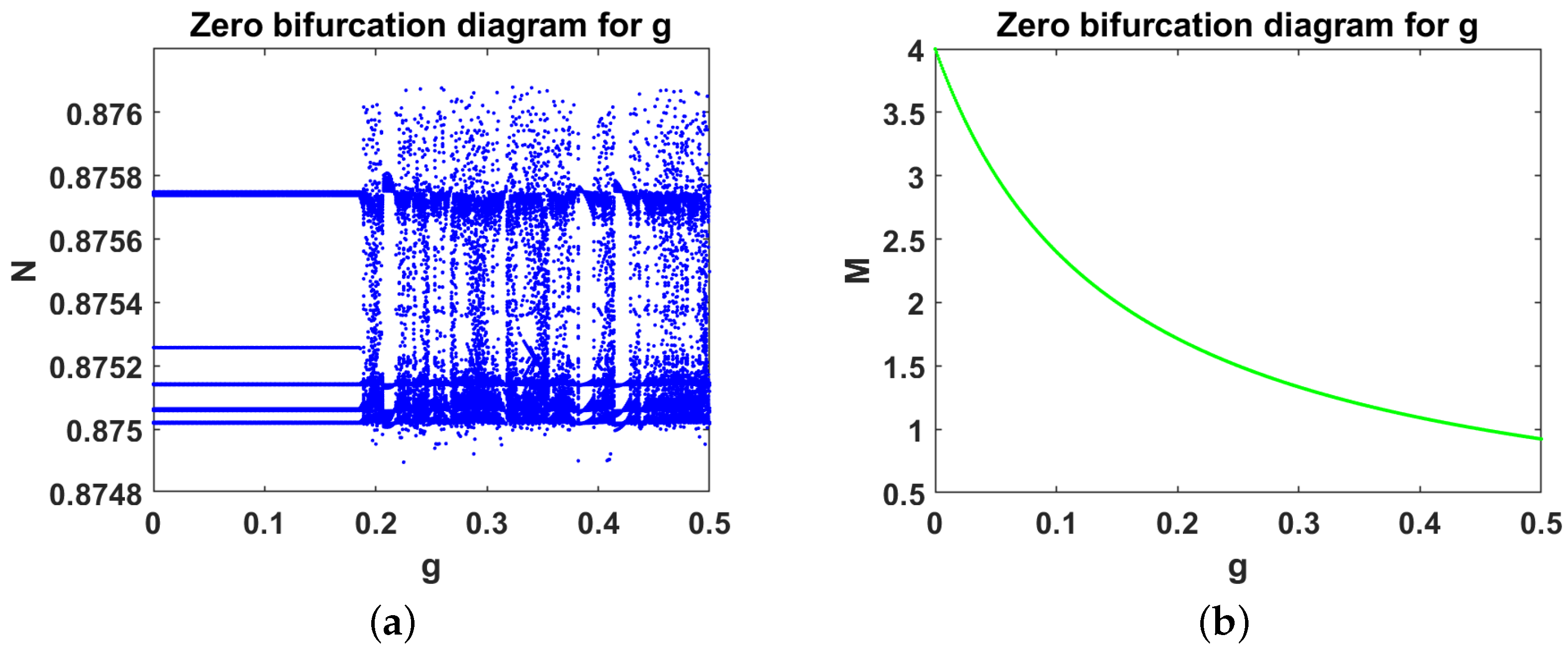
The numerical model equations derived in Section 3 and Section 4 are simulated, and the results are presented herewith. Maple (2020 version) software and MATLAB (2020a version) ODE45 solver were used for the simulations of the model equations. The findings obtained from the simulations of the model Equation (1) discerned the complex dynamical behavior of the breast cancer cells’ population in the co-existence of both normal (host) and immune cells. In addition, the impact of the given fixed parameters that asymptotically stabilized the model Equation (1) and its stability lost via zero and Hopf bifurcations were examined.

Table 1. The fixed parameters used in zero and Hopf bifurcations.

Parameter	Value	Unit
${\alpha }_1$	0.7	day${}^{-1}$
${\mu }_1$	0.8	day${}^{-1}$
${\varphi }_1$	0.1	day${}^{-1}$
${\alpha }_2$	0.98	day${}^{-1}$
${\mu }_2$	0.4	day${}^{-1}$
${\gamma }_1$	0.8	day${}^{-1}$
$\rho$	0.3	day${}^{-1}$
$\omega$	0.3	day${}^{-1}$
${\gamma }_2$	0.29	day${}^{-1}$
${\mu }_3$	0.15	day${}^{-1}$

enlists the values of all fixed parameters used in the stability or bifurcations analysis. All values in Table 1 are taken from [9].

Case 1. 

Complete absence of tumor cells We took ${\varphi }_2=0.5,s=0.6>s_0$ and varied g. Theorem 6 was used to obtain $s_0\simeq 0.27$. Equation (16) was used to obtain $g_0=0.15521$ with $\Delta \simeq 2.257>0$, thereby achieving a free equilibrium point $E_0=\left(0.875,0,1.966\right)$. The associated Jacobian matrix $J\left(E_0\right)$ produced a zero eigenvalue $\left({\lambda }_1=0\right)$ and two negative eigenvalues ${\lambda }_2=-0.7,$ ${\lambda }_3\simeq -0.782.$ Theorem 6 was used in the model Equation (1) to obtain a generic saddle-node bifurcation for $g=g_0.$ Interestingly, $E_0$ changed its stability via the transcritical bifurcation when g crossed the critical value $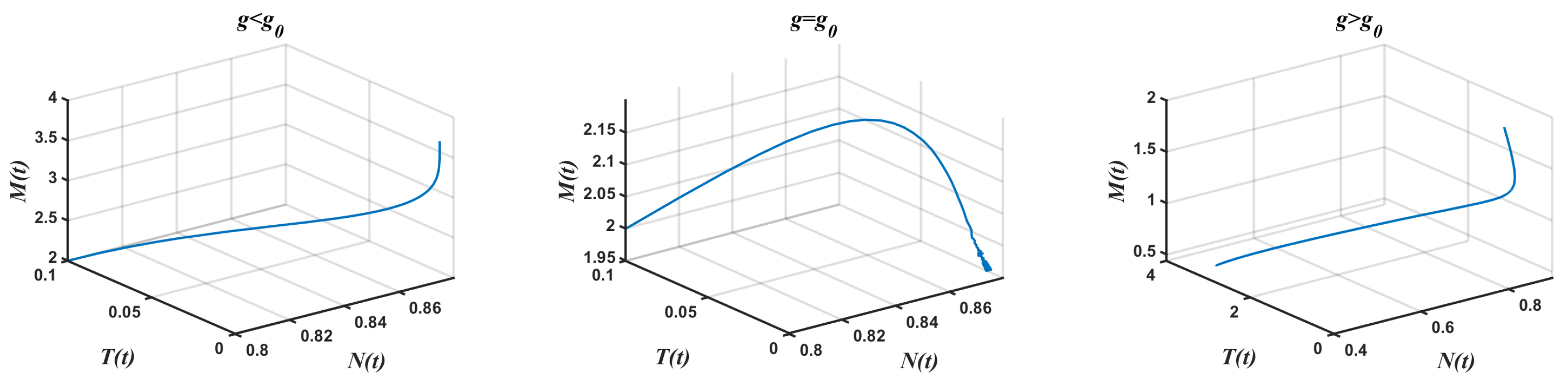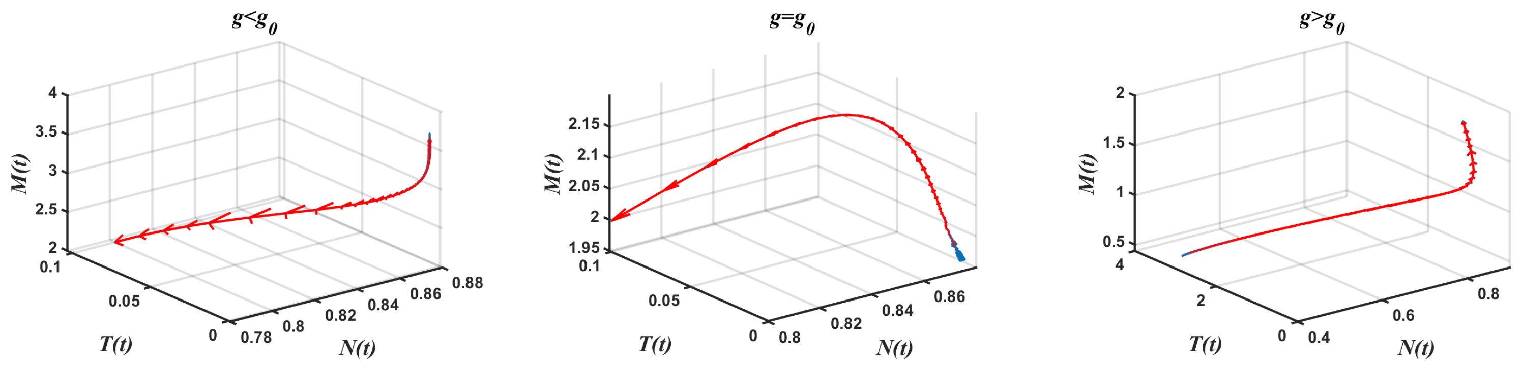g_0.$

Figure 2 displays the glucose parameter-dependent transcritical bifurcation of the model Equation (1). It was observed that $E_0$ is a stable point for $g<g_0$ (Figure 2a). With the increase of g, the dynamics of the cells population became chaotic for $g>g_0$, indicating that the existing glucose in the breast cancer patient’s body can add significant risks and make the normal cells highly unstable when the tumor cells are absent. In addition, excessive contents of g in the patient body can lead to a quick chaos saturation in the normal cells population. It can be argued that glucose might have an influence on the logistic growth of the normal cells (Figure 2a). From the biological perspective, it can be inferred that the presence of glucose in the breast cancer patient’s body may cause a mutation of the normal cells, forcing them to grow uncontrollably and thus leading to carcinoma [24,34]. Figure 2b clearly shows that glucose excess has an appreciable influence on the dynamical behavior of the immune cells, resulting in a decrease in the efficiency of the immune system [20,21] without entering in any chaotic regime. This observation can be ascribed to various factors such as the nature of the immune cells that die and reproduce daily [24,25]. In short, the immune cells might not reach the chaotic state irrespective of the excess glucose level in the cancer patient’s blood. If the immune cells reach a chaotic state, this is considered as a risk factor wherein the immune cells might be transferred to the cancer immune cells [9]. The corresponding parametric solutions and phase plots of the model shown in Equation (1) as a function of g are depicted in Figure 3 and Figure 4, respectively. The results showed that $E_0$ is a stable point when $g<g_0$; however, its stability is lost gradually with the increase of g.

Case 2. 

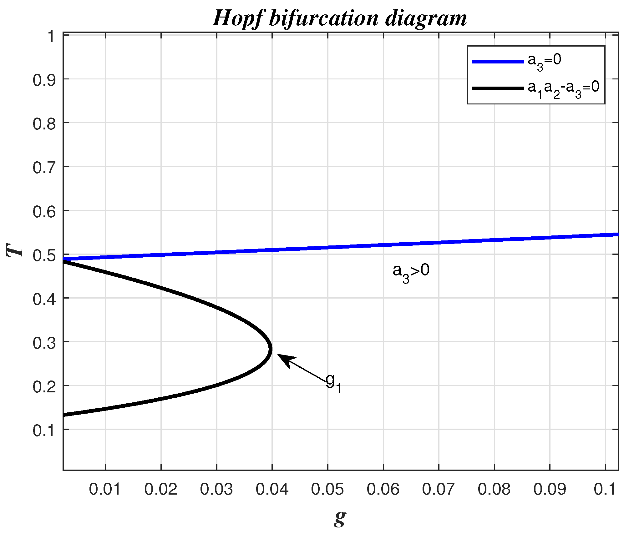
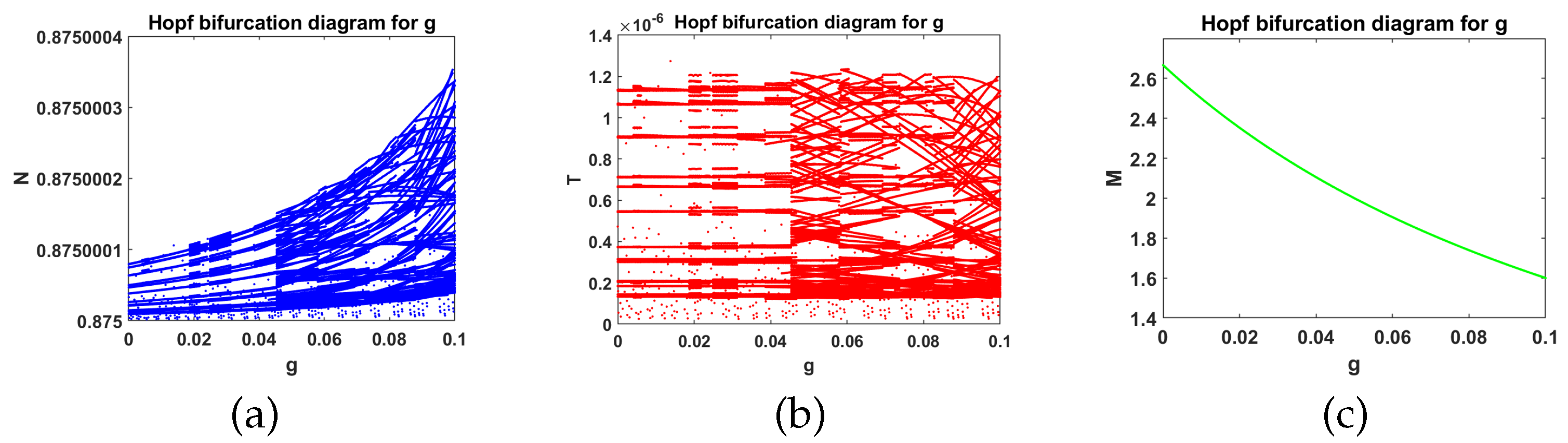
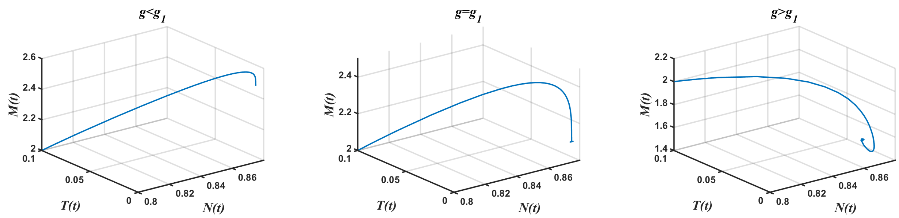
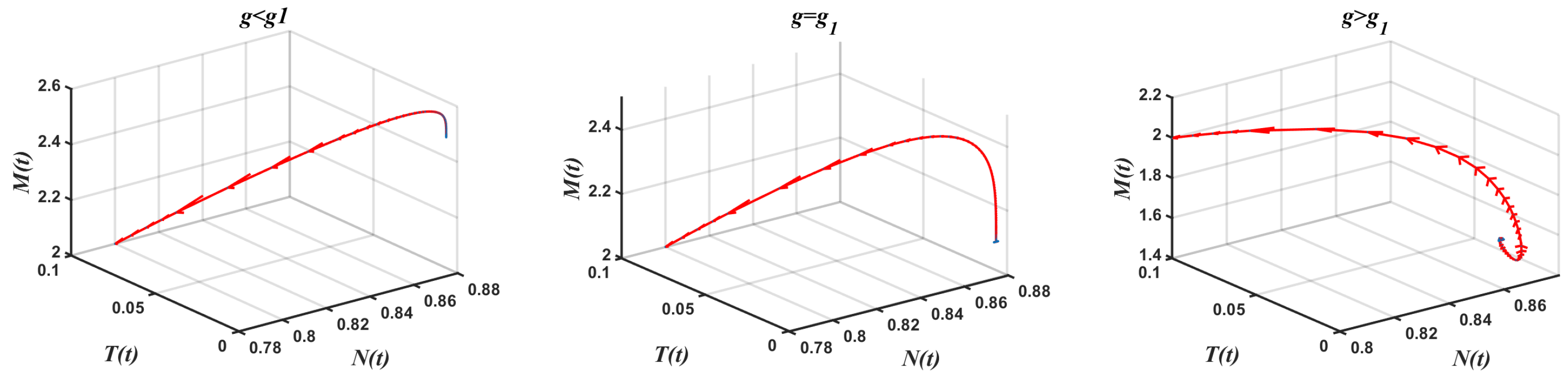
In the presence of tumor cells In this case, the simulation is carried out by taking ${\varphi }_2=0.1, \rho =0.8$, $s=0.4$, and other parameters have the same fixed values as indicated in Table 1. According to Theorem 9, $J\left(E_3\right)$ had a pair of pure imaginary eigenvalues on the imaginary axis, and other roots lie on the left half-plane when the conditions given by Equation (33) are violated. The achieved critical Hopf bifurcation satisfied Equation (34) at $g=g_1=0.03941$. In addition, the coexistence equilibrium point $E_3=\left(0.8377,0.2983,1.2298\right)$ was obtained. The Jacobian matrix $J\left(E_3\right)$ had a negative real eigenvalue ${\lambda }_1=-0.6665$ with a pair of pure imaginary eigenvalues ${\lambda }_{2,3}=\pm 0.3115i,$ $i=\sqrt{-1}.$ According to Theorem 9, the model Equation (1) produced a Hopf bifurcation when $g=g_1.$ Furthermore, $E_3$ changed its stability via the Hopf bifurcation when g crossed the critical parameter $g_1.$

Figure 5 illustrates the Hopf bifurcation diagram for $g\in \left(0,0.1\right).$ The area under the blue line satisfied the solutions of the inequalities $a_1>0$ and $a_3>0$ given in Equation (34). The critical value of $g=g_1$ was positioned on the black line inside the region in which $a_1{a}_2-a_3=0$ in Equation (34) was satisfied. In brief, the emergence of Hopf bifurcation at $E_3$ for $g\in \left(0,0.1\right)$ was clearly evidenced.

Figure 6 displays the appearance of stable point $E_3$ for various values of $g<g_1$ and the stability lost via the Hopf bifurcation for $g>g_1.$ The normal and tumor cells population (Figure 6a,b were found to be stable when the glucose factor remained below its critical value $g_1.$ The attractor regions in the figure revealed that $E_3$ altered its stability for $g>g_1$, and a perturbation appeared in the normal and tumor cells population with the increase of g. Furthermore, the glucose excess was shown to cause a perturbation (chaos) in the normal and tumor cells, which can be attributed to the strong interactions among the normal and tumor cells in the patient’s body. A comparison between the effects of glucose excess on the behavior of the immune cells (Figure 6c) showed that the tumor cells had strong competition with other cells.

The effect of glucose excess on the immune cells in the absence of the tumor cells (Figure 2b) was found to negatively affect the efficiency of the immune system. In addition, the immune cells were decreased dramatically compared to the behavior of cells, as shown in Figure 2b. From a biological viewpoint, the reduction of the cells can refer to the interaction between the immune cells and tumor cells under the excess of glucose wherein one of the responsibilities of the immune system is to attack the pathogen or any foreign cells. Despite the presence of positive side effects from the behavior of the immune cells under the existence of the tumor cells, with an excess of glucose, the immune system did not attain the chaos. This observation clearly indicated that it is possible to modify the dynamical behavior of the cells and avoid their transfer to the cancer immune cells, thereby reducing the breast cancer patient’s health risks [9]. Figure 7 and Figure 8 represent the parametric solution and the phase portraits, respectively, corresponding to Figure 6, which displayed the different stability behavior of the point $E_3$ around $g_1.$ The point $E_3$ was found to be stable for $g<g_1$ and then lost its stability via the Hopf bifurcation when $g=g_1$ and g became greater than $g_1$.

6. Conclusions

We proposed a mathematical model for breast cancer in the presence of excess blood glucose risk factors. To indicate the symmetry between the biological meaning and the mathematical modeling of the cells’ behavior, the numerical model equations were simulated to determine the complex dynamics of host, immune, and cancer cells population that lead to immune system failure for the patient. The results revealed the existence of different equilibrium points related to the tumor-free ($E_0$), type 1 dead ($E_1$), type 2 dead ($E_2$), and coexistence ($E_3$) for various glucose parameters. The local stabilities of these equilibrium points were analyzed in depth to determine the excess glucose-stimulated effects in the breast cancer tissues. The zero bifurcation (generic saddle-node bifurcation) at $E_0$ was examined, wherein a new strategy was followed to detect such bifurcation based on the sums of the principal minors of $J\left(E_0\right)$. It was demonstrated that $E_0$ produces a transcritical bifurcation for g values greater than $g_0$. In addition, the occurrence of Hopf bifurcation at $E_3$ needed some sufficient and necessary conditions depending on the Hurwitz determinants expressed in terms of a semi-algebraic system. The model results revealed diverse complex dynamics such as Hopf bifurcation and chaos with the increase of g beyond a certain threshold. An outbreak was evidenced in the normal and tumor cells population when the blood glucose value of the breast cancer patient exceeded a certain critical value. Despite the instability of the immune cells for g above the critical value, they did not pass through any chaotic regime, which was ascribed to the nature of the damage caused by excess glucose to normal cells and tumors only wherein the immune response provided a stimulus to the creation of new cancer cells at the expense of normal cells via the competitive mechanisms. The numerical simulation results validated the analytical predictions. The results of this study open the door to several biological, medical and mathematical studies that are contributing to raising awareness of cancer risk and its treatment. In the end, it is asserted that the present comprehensive model for breast cancer with added glucose risk factors may constitute a basis to study other types of the cancer risks in the presence of external factors.

References

1. Dolatkhah, M.; Hashemzadeh, N.; Barar, J.; Adibkia, K.; Aghanejad, A.; Barzegar-Jalali, M.; Omidi, Y. Graphene-based multifunctional nanosystems for simultaneous detection and treatment of breast cancer. Colloids Surf. B Biointerfaces 2020, 193, 111104. [Google Scholar] [CrossRef] [PubMed]
2. Santos, J.M.; Hussain, F. Higher glucose enhances breast cancer cell aggressiveness. Nutr. Cancer 2020, 72, 734–746. [Google Scholar] [CrossRef] [PubMed]
3. Sakaguchi, A.Y.; Spolador, L.H.; de Sousa Pereira, N.; Bocchi, M.; Fernandes, C.Y.; de Oliveira Pinsetta, M.; Munuera, M.D.; Moretto, S.L.; Fuzinatto, I.M.; de Castro, V.D.; et al. Breast cancer and nutrition: Interplay between diet and cancer prevention. Biosaúde 2020, 21, 87–99. [Google Scholar]
4. Sung, H.; Ferlay, J.; Siegel, R.L.; Laversanne, M.; Soerjomataram, I.; Jemal, A.; Bray, F. Global cancer statistics 2020: GLOBOCAN estimates of incidence and mortality worldwide for 36 cancers in 185 countries. CA Cancer J. Clin. 2021, 71, 209–249. [Google Scholar] [CrossRef] [PubMed]
5. Ku-Carrillo, R.A.; Delgadillo, S.E.; Chen-Charpentier, B.M. A mathematical model for the effect of obesity on cancer growth and on the immune system response. Appl. Math. Model. 2016, 40, 4908–4920. [Google Scholar] [CrossRef]
6. Dehingia, K.; Yao, S.W.; Sadri, K.; Das, A.; Sarmah, H.K.; Zeb, A.; Inc, M. A study on cancer-obesity-treatment model with quadratic optimal control approach for better outcomes. Results Phys. 2022, 42, 105963. [Google Scholar] [CrossRef]
7. Alharbi, S.A.; Rambely, A.S. Dynamic behaviour and stabilisation to boost the immune system by complex interaction between tumour cells and vitamins intervention. Adv. Differ. Equ. 2020, 2020, 412. [Google Scholar] [CrossRef]
8. Admon, M.R.; Maan, N. Modelling tumor growth with immune response and drug using ordinary differential equations. Jurnal Teknologi 2017, 79, 49–56. [Google Scholar] [CrossRef] [Green Version]
9. Mufudza, C.; Sorofa, W.; Chiyaka, E.T. Assessing the effects of estrogen on the dynamics of breast cancer. Comput. Math. Methods Med. 2012, 2012, 473572. [Google Scholar] [CrossRef] [Green Version]
10. Oke, S.I.; Matadi, M.B.; Xulu, S.S. Optimal control analysis of a mathematical model for breast cancer. Math. Comput. Appl. 2018, 23, 21. [Google Scholar]
11. Debbouche, N.; Ouannas, A.; Grassi, G.; Al-Hussein, A.B.A.; Tahir, F.R.; Saad, K.M.; Jahanshahi, H.; Aly, A.A. Chaos in Cancer Tumor Growth Model with Commensurate and Incommensurate Fractional-Order Derivatives. Comput. Math. Methods Med. 2022, 2022, 5227503. [Google Scholar] [CrossRef] [PubMed]
12. Abd-Rabo, M.A.; Zakarya, M.; Alderremy, A.A.; Aly, S. Dynamical analysis of tumor model with obesity and immunosuppression. Alex. Eng. J. 2022, 61, 10897–10911. [Google Scholar] [CrossRef]
13. Fadaka, A.; Ajiboye, B.; Ojo, O.; Adewale, O.; Olayide, I.; Emuowhochere, R. Biology of glucose metabolization in cancer cells. J. Oncol. Sci. 2017, 3, 45–51. [Google Scholar] [CrossRef]
14. Vander Heiden, M.G.; Cantley, L.C.; Thompson, C.B. Understanding the Warburg effect: The metabolic requirements of cell proliferation. Science 2009, 324, 1029–1033. [Google Scholar] [CrossRef] [PubMed] [Green Version]
15. Chen, M.C.; Hsu, L.L.; Wang, S.F.; Hsu, C.Y.; Lee, H.C.; Tseng, L.M. ROS Mediate xCT-Dependent Cell Death in Human Breast Cancer Cells under Glucose Deprivation. Cells 2020, 9, 1598. [Google Scholar] [CrossRef]
16. Wardi, L.; Alaaeddine, N.; Raad, I.; Sarkis, R.; Serhal, R.; Khalil, C.; Hilal, G. Glucose restriction decreases telomerase activity and enhances its inhibitor response on breast cancer cells: Possible extra-telomerase role of BIBR 1532. Cancer Cell Int. 2014, 14, 60. [Google Scholar] [CrossRef] [Green Version]
17. Krętowski, R.; Borzym-Kluczyk, M.; Stypułkowska, A.; Brańska-Januszewska, J.; Ostrowska, H.; Cechowska-Pasko, M. Low glucose dependent decrease of apoptosis and induction of autophagy in breast cancer MCF-7 cells. Mol. Cell. Biochem. 2016, 417, 35–47. [Google Scholar] [CrossRef] [Green Version]
18. Barbosa, A.M.; Martel, F. Targeting glucose transporters for breast cancer therapy: The effect of natural and synthetic compounds. Cancers 2020, 12, 154. [Google Scholar] [CrossRef] [Green Version]
19. Sun, S.; Sun, Y.; Rong, X.; Bai, L. High glucose promotes breast cancer proliferation and metastasis by impairing angiotensinogen expression. Biosci. Rep. 2019, 39, BSR20190436. [Google Scholar] [CrossRef] [Green Version]
20. Shomali, N.; Mahmoudi, J.; Mahmoodpoor, A.; Zamiri, R.E.; Akbari, M.; Xu, H.; Shotorbani, S.S. Harmful effects of high amounts of glucose on the immune system: An updated review. Biotechnol. Appl. Biochem. 2020, 68, 404–410. [Google Scholar] [CrossRef]
21. Von Ah Morano, A.E.; Dorneles, G.P.; Peres, A.; Lira, F.S. The role of glucose homeostasis on immune function in response to exercise: The impact of low or higher energetic conditions. J. Cell. Physiol. 2020, 235, 3169–3188. [Google Scholar] [CrossRef]
22. O’Mahony, F.; Raz, I.M.; Pedram, A.; Harvey, B.J.; Levin, E.R. Estrogen modulates metabolic pathway adaptation to available glucose in breast cancer cells. Mol. Endocrinol. 2012, 26, 2058–2070. [Google Scholar] [CrossRef] [PubMed]
23. Sun, Y.S.; Zhao, Z.; Yang, Z.N.; Xu, F.; Lu, H.J.; Zhu, Z.Y.; Shi, W.; Jiang, J.; Yao, P.P.; Zhu, H.P. Risk factors and preventions of breast cancer. Int. J. Biol. Sci. 2017, 13, 1387. [Google Scholar] [CrossRef] [PubMed] [Green Version]
24. Cooper, G.M.; Hausman, R.E.; Hausman, R.E. The Cell: A Molecular Approach; ASM Press: Washington, DC, USA, 2007; Volume 4, pp. 649–656. [Google Scholar]
25. Murphy, K.M.; Weaver, C. Janeway’s Immunobiology: Ninth International Student Edition; Garland Science, Taylor & Francis Group, LLC: New York, NY, USA, 2017. [Google Scholar]
26. Bronshtein, I.N.; Semendyayev, K.A. Handbook of Mathematics; Springer Science & Business Media: Berlin/Heidelberg, Germany, 2013. [Google Scholar]
27. Tilekar, K.; Upadhyay, N.; Iancu, C.V.; Pokrovsky, V.; Choe, J.Y.; Ramaa, C.S. Power of two: Combination of therapeutic approaches involving glucose transporter (GLUT) inhibitors to combat cancer. Biochim. Biophys. Acta (BBA)-Rev. Cancer 2020, 1874, 188457. [Google Scholar] [CrossRef] [PubMed]
28. Pliszka, M.; Szablewski, L. Glucose transporters as a target for anticancer therapy. Cancers 2021, 13, 4184. [Google Scholar] [CrossRef] [PubMed]
29. Zhou, J.; Zhu, J.; Yu, S.J.; Ma, H.L.; Chen, J.; Ding, X.F.; Chen, G.; Liang, Y.; Zhang, Q. Sodium-glucose co-transporter-2 (SGLT-2) inhibition reduces glucose uptake to induce breast cancer cell growth arrest through AMPK/mTOR pathway. Biomed. Pharmacother. 2020, 132, 110821. [Google Scholar] [CrossRef] [PubMed]
30. Stefano, B.; Desmarchelier, D. Local bifurcations of three and four-dimensional systems: A tractable characterization with economic applications. Math. Soc. Sci. 2019, 97, 38–50. [Google Scholar]
31. Cardin, P.T.; Llibre, J. Transcritical and zero-Hopf bifurcations in the Genesio system. Nonlinear Dyn. 2017, 88, 547–553. [Google Scholar] [CrossRef] [Green Version]
32. Weber, A. Deciding Hopf bifurcations by quantifier elimination in a software-component architecture. J. Symb. 2000, 30, 161–179. [Google Scholar]
33. Hong, H.; Liska, R.; Steinberg, S. Testing stability by quantifier elimination. J. Symb. Comput. 1997, 24, 161–187. [Google Scholar] [CrossRef]
34. Hatami, M.; Akbari, M.E.; Abdollahi, M.; Ajami, M.; Jamshidinaeini, Y.; Davoodi, S.H. The relationship between intake of macronutrients and vitamins involved in one carbon metabolism with breast cancer risk. Sci. Inf. Database 2017, 75, 56–64. [Google Scholar]
Figure 1. The cells’ population competition in the proposed model.
Mathematics 10 03640 g001
Figure 2. Transcritical bifurcation diagram of model (1) with respect to glucose parameter g where g ( 0 , 0.5 ) . (a) represents the effect of glucose, g, on the behavior of normal cells denoted by N. (b) shows the glucose impact on immune cells denoted by M.
Mathematics 10 03640 g002
Figure 3. Parametric solutions of model (1) for various g-values corresponding to Figure 2.
Mathematics 10 03640 g003
Figure 4. Phase portraits of model (1) for various g-values corresponding to Figure 2.
Mathematics 10 03640 g004
Figure 5. The conditions in (34) are illustrated. When g = g 1 , the model (1) has a coexistence equilibrium point E 3 = ( 0.8377 , 0.2983 , 1.2298 ) . .
Mathematics 10 03640 g005
Figure 6. The emergence of Hopf bifurcation at E 3 for normal cells N, tumor cells T, and immune cells M, respectively, with respect to glucose parameter g where g ( 0 , 0.1 ) . (a) The effect of glucose on the normal cells. (b) The effect of glucose on the tumour cells. (c) The effect of glucose on the immune cells.
Mathematics 10 03640 g006
Figure 7. Parametric solutions of model (1) for various g values corresponding to Figure 5.
Mathematics 10 03640 g007
Figure 8. Phase portraits of model (1) for various g values corresponding to Figure 5.
Mathematics 10 03640 g008