A Deep Network-Based Trade and Trend Analysis System to Observe Entry and Exit Points in the Forex Market

Abstract

In the Forex market, trend trading, where trend traders identify trends and attempt to capture gains through the analysis of an asset’s momentum in a particular direction, is a great way to profit from market movement. When the price of currency is moving in one either of the direction such as; up or down, it is known as trends. This trend analysis helps traders and investors find low risk entry points or exit points until the trend reverses. In this paper, empirical trade and trend analysis results are suggested by two-phase experimentations. First, considering the blended learning paradigm and wide use of deep-learning methodologies, the variants of long-short-term-memory (LSTM) networks such as Vanilla-LSTM, Stacked-LSTM, Bidirectional-LSTM, CNN-LSTM, and Conv-LSTM are used to build effective investing trading systems for both short-term and long-term timeframes. Then, a deep network-based system used to obtain the trends (up trends and down trends) of the predicted closing price of the currency pairs is proposed based on the best fit predictive networks measured using a few performance measures and Friedman’s non-parametric tests. The observed trends are compared and validated with a few readily available technical indicators such as average directional index (ADX), rate of change (ROC), momentum, commodity channel index (CCI), and moving average convergence divergence (MACD). The predictive ability of the proposed strategy for trend analysis can be summarized as follows: (a) with respect to the previous day for short-term predictions, AUD:INR achieves 99.7265% and GBP:INR achieves 99.6582% for long-term predictions; (b) considering the trend analysis strategy with respect to the determinant day, AUD:INR achieves 98.2906% for short-term predictive days and USD:INR achieves an accuracy of trend forecasting with 96.0342%. The significant outcome of this article is the proposed trend forecasting methodology. An attempt has been made to provide an environment to understand the average, maximum, and minimum unit up and/or downs observed during trend forecasting. In turn, this deep learning-based strategy will help investors and traders to comprehend the entry and exit points of this financial market.

1. Introduction

In the Forex financial market, forecasting and providing a platform to make correct and accurate decisions towards investment is the most challenging affair for investors, brokers, and business houses. Understanding the sentiment of markets and economic growth of countries are the potential inputs to analyze this market and ensure that the assets invested must give measurable value and maximum return on investment. The key objective of focusing on forecasting or predicting the currency exchange rate between countries is to help investors, brokers, and traders through an automated system which can produce informed or guided decisions for minimizing the risk of investment along with maximizing returns on the invested amount leading to a well-produced trading strategy [1,2]. The most commonly used methods focus on: (a) purchasing power parity, the idea that there should be no purchasing and selling of the same asset in different markets to extract the best profit, which exploits the short-lived variations in the price of a similar asset in different country’s markets; (b) relative economic strength, which measures the economic strength of the country with respect to their growth and is basically used to attract foreign investors; (c) econometric models, which gather the factors influencing the forecasting of exchange rates based on economic theory such as statistical and mathematical methods, and the variables which can influence the exchange rate are also taken into consideration [3,4].

The recent trend of embracing the digital medium of analyzing financial assets in business industries has set ample opportunities for the research community and information technology industries to design and develop automated financial applications or models which can understand financial market sentiments and are able to deliver accurate and smart decisions with emerging technologies. Though traditional models of financial market analysis are doing well based on historical data, the short shelf life of these models is limiting their use and effectiveness. Understanding the patterns of the financial market for making decisions is also a motivating factor for researchers, and they are now studying the various patterns of this financial market through trend analysis [5,6]. The forecasting process of the Forex financial market is a risky and tedious task; therefore, researchers require detailed insight into such practices when developing any trading and/or trend analysis model.

This study is also popularly known as spend forecasting, aiming to provide optimal decisions and observation patterns based on historical data, the current situation or environment, and predictive analytics. This trend or spend forecasting provides the solution for ‘What next?’ for a specific time frame of investment, such as daily, monthly, quarterly, or yearly. In short, trend analysis examines the financial market and economic conditions and identifies two categories of trends, up trends or bull markets and down trends or bear markets [2,5,6,7]. Up trends represent the increase in asset prices and predicted growth over a given amount of time, and, in this trend, the investors are eager to catch the wave of investing to earn profits. In contrast, down trends direct the bad economic conditions of the markets, leading investors to become more conservative and not interested in investing. To summarize, this trend analysis provides a direction of the profits/losses for the assets, and it makes the decision-making approach straightforward for investors and business industries. The various tools and techniques of machine learning and deep learning algorithms now play a vital role in predicting the currency exchange price of each money pair during the classification process, and with the help of supervised learning techniques, market trends (up trends and down trends) are being predicted to help investors and traders make the correct decisions regarding Forex transactions [5,6,8,9].

Deep network has established a new blended learning paradigm by exploiting the architecture and functionalities of artificial intelligence and machine learning strategies in the domain of financial market analysis. The strong underlying methodologies of deep network based on mathematical and computational mechanisms have become a great challenge to researchers, and people are still trying to develop computational models based on this deep network; hence, the development of an application-specific network is a challenge that needs to be addressed [10,11,12]. Deep network has shown its performance in categorization and prediction domains by drawing curvy or straight lines through data points to categorize datasets or predict the value at which a trend will increase or decrease [13,14,15].

Overall, current currency exchange rate prediction and identification of trends present a good opportunity to study this financial market and the ability of deep learning with respect to processing many features with inbuilt filtering architecture; furthermore, the methods used are skilled in dealing with unstructured data and complex problems, showing their effectiveness to focus on this area of research. Motivated by the efficiency of deep learning techniques, this study poses an empirical attempt to obtain currency pair trading prices as well as a trend analysis strategy to identify the up trends and down trends of this market for both short-term (15 days) and long-term (60 days) prediction of horizons. The literature suggests the use of long short-term memory (LSTM) [16,17,18], one of the most widely used deep learning strategies, for the prediction of this financial market. This further motivated us to utilize the variants of LSTM forecasting networks, as this could lead to improved results.

Based on the above context, this work makes the following contributions:

• Five variants of LSTM, such as Vanilla-LSTM, Stacked-LSTM, Bidirectional-LSTM, Convolutional Neural Network-LSTM (CNN-LSTM), and Conv-LSTM, are used as trading strategies [16,17,18,19,20,21]. The performance of these five models is recorded with respect to explained variance score (EVS), maximum error (ME), mean squared error (MSE), and R-square (R2) [22];
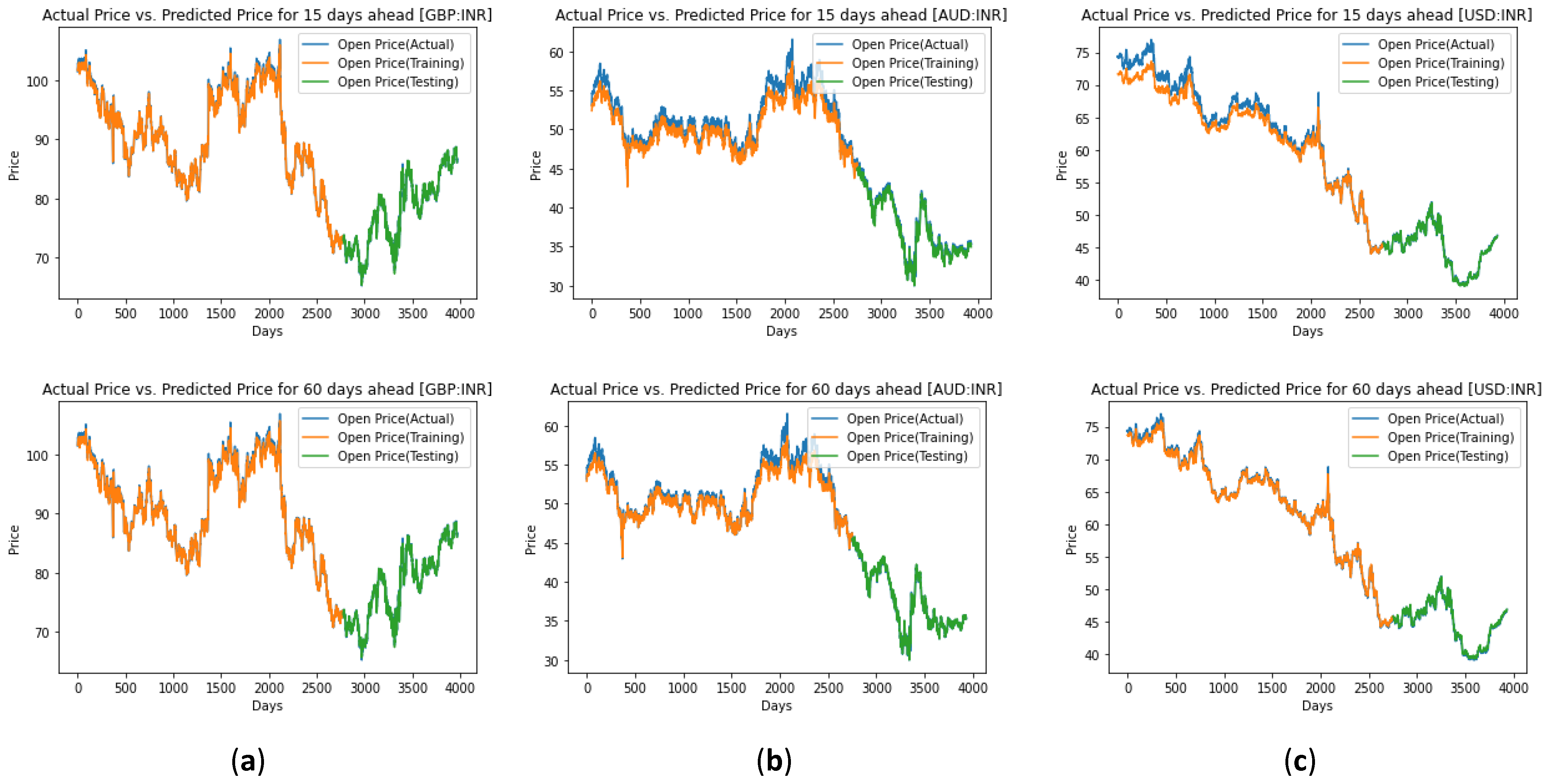
• Prediction curves are plotted to visualize the predictive performance. The best fit models are obtained with respect to the prediction period for all three currency pairs used for experimentation;
• To attain a holistic view of the results obtained using predictive models, statistical validation is performed using Friedman’s non-parametric statistical test [23,24];
• A deep learning-based system for obtaining the trends of the currency pair is proposed based on the selling or buying of currencies, focusing on the previous day and the determinant day (a few days ahead as per user input) to observe the trends for a certain day (date) for both short-term and long-term forecasting horizons;
• Readily available technical indicators such as average directional index (ADX), rate of change (ROC), momentum, commodity channel index (CCI), and moving average convergence divergence (MACD) [25,26,27] are used to observe the trends on those three-currency pair datasets;
• A straightforward comparison is made between the proposed trend analysis strategy, actual trends observed on original datasets, and the trends observed based upon those tools;
• In order to handle risks in this financial market, an attempt is made to help investors and traders to identify not only the trends but also the strength of the trends with respect to the average, maximum, and minimum number of units, either up or down, observed during the up trends or down trends and put them in a position to understand the profitable entry and exit points and provide buying or selling opportunities. Finally, the average computational time for all the algorithms used for trading and trend analysis are presented.

This paper is organized as follows: a literature survey on forecasting models based on variants or hybrids of LSTM, along with a few studies conducted on trend analysis, are discussed in Section 2. The methodologies adopted for experimentation and the proposed trend analysis strategies are discussed in Section 3. Section 4 focuses on the experimental setup, and the experimentation, evaluation, and results in the analysis of this research are discussed in Section 5. Finally, Section 6 concludes the work with future scope.

2. Literature Survey

This section provides detailed study on Forex market analysis focusing on existing research conducted on LSTM and the hybrid forms of LSTM-based trading models. In addition, a few proposed trend analysis methods are also discussed. An ensemble approach called LSTM-B, integrating the LSTM neural network and bagging ensemble learning strategy, was proposed by Shaolong Sun et al. [28] to obtain accuracy in the Forex market and improve the profit of exchange rate trading. This ensemble deep learning approach yields better performance when compared with other benchmarks, which may or may not include bagging ensemble learning methods. Salman Ahmed et al. [16] proposed an integrated system which uses Forex Loss Function (FLF) in an LSTM (FLF-LSTM) which reduces the differences between actual and predictive averages of Forex candles. The authors compared the proposed approach with a recurrent neural network (RNN)-based prediction system and the auto-regressive integrated moving average and found a minimal error with respect to open, high, and low prices, respectively. To analyze trade data, Mei-Li Shen et al. [17] developed an effective trade forecasting method which works on a neural network with LSTM. The authors proposed multivariate LSTM-based techniques which extract the progressive changes from trade data and result in an effective trade forecasting system. M.S. Islam and E. Hossain [29] proposed a new model with the combination of Gated Recurrent Unit (GRU) and LSTM methods, which works for time series prediction and predicts the future closing price of Forex currency. The performance of the model was validated and compared with basic LSTM, basic GRU, and simple moving average (SMA), and it was observed that the GRU-LSTM model shows better results. Gang Wang et al. [30] proposed an ensemble method which uses adaptive linear sparse random subspace (ALS-RS) based on the effect of shallow and deep features. Here, the shallow feature is constructed manually using expert knowledge, whereas the deep feature is extracted automatically using bidirectional GRU. Based on the deep learning framework, a model was proposed by Shuigen Yang [14] to predict financial indicator values. His model uses LSTM as a benchmark prediction model and is used to forecast the financial risk in the financial sector. Yong Lin et al. [31] applied the multifractal detrended cross-correlation analysis (MF-DCCA) method to examine the cross-correlation behavior between the USD/CNY exchange rate and the Baidu index (BI). The authors proposed a hybrid deep learning model, WOASTL-BI-LSTM, to predict UCER returns, where BI is used as a potential predictor to predict UCER. Sangjin Park and Jae-Suk Yang [18] presented a deep learning model based on the LSTM network to predict economic growth. Along with this, the authors also used an interpretable machine learning model which derives economic growth patterns and crises using the eXplainable AI (XAI) framework. An LSTM and GRU-based hybrid crypto-currency prediction framework was proposed by Mohil Mahesh Kumar Patel et al. [32]. The proposed framework focused on only two crypto-currencies, namely Litecoin and Monero. Saúl Alonso-Monsalve et al. [27] explored the use of a neural network with a convolutional component in the domain to classify the trends of crypto-currency exchange rates. The authors compared the performance of the proposed work with different network architectures and found convolutional LSTM neural networks significantly outperformed all other methods.

In Forex market prediction, the prediction of market trends and automated trading are important factors for stakeholders, and recent trend forecasting of financial time series data is considered a top choice for finance researchers. Here, a few studies on trend forecasting are discussed to obtain better insight into this domain of research. A comprehensive study was presented by Omer Berat Sezer et al. in ref. [15], which includes the application of variants of deep learning strategies, such as convolutional neural networks (CNNs), deep belief networks (DBNs), and LSTMs, in the field of financial time series forecasting. T. Tokár and D. Horváth [33] analyzed the local trends used for currency trading. With different time delays, the authors introduced several statistical quantities to examine the role of a single temporal discretized trend or a multitude of grouped trends. Hossein Talebi et al. [6] proposed a classifier for identifying up, down, and sideways trends in the Forex market. The authors used an ensemble classifier to obtain better results than the individual classifier used for trend analysis. Yunli Lee et al. [34] extracted the features from trend patterns to predict the next day’s movement of trends. To obtain long-term trends and short-term movements of stock market data, Salim Lahmiri [35] introduced the variational mode decomposition (VMD) method for signal processing which is used to decompose stock market data into a finite set of modes.

The author also used detrended fluctuation analysis (DFA) and range scale (R/S) to evaluate the Hurst exponent in each mode obtained from VMD. Javier Sandoval et al. [36] presented a graphical picture which fully depicts the price–time–volume dynamics in a limit order book and the required trend is predicted by clustering techniques. For trading in the financial market, Erik Bartoš et al. [37] introduced multidimensional string objects. The authors showed how new object properties could change the statistics of predictors, which can help to regenerate candidates for modeling time series systems. In many forecasting algorithms, the physical time scale is used for studying price movement in financial markets. However, the use of a physical time scale may cause risk in the market; hence, Adesola Adegboye et al. [38,39,40] proposed a new approach, namely directional change (DC), which uses an event-based time scale in 2017, 2019, and 2021. This approach represents the data in upward directional change and downward directional change. The trends can also be expressed in DC events and overshoot (OS) events. The authors also attempted to predict the reverse trend to increase profitability using a genetic programming algorithm, which includes linear and non-linear relationships between the length of DC and OS events in a particular dataset. In 2019 [39], they extended their work based on the DC approach for sampling market data and the extraction of trends in financial time series by replacing the time-based format with an event-based format. The authors explored different machine learning algorithms and tested the performance. They used particle swarm optimization and the shuffled frog leaping algorithm on 36 different datasets from four different currency pairs and found statistically improved profitability on DC-based trading. In 2021, the same authors [40] proposed a DC-based framework with machine learning algorithms to predict the reverse trend. The proposed approach was able to return high profits with reduced risk. The work was compared with 10 benchmark datasets with technical analysis and bye-and-hold for both DC and non-DC-based approaches. In the Forex market, existing trading systems include technical analysis with crisp technical indicators for buy or sell signals. This approach can be replaced with the fuzzy approach, which generates buy or sell signals with a fuzzy membership function. To achieve an efficient trend in the Forex market, Alireza Sadeghi et al. [41] presented a combined approach which is based on an ensemble multi-class support vector machine (EmcSVM) and fuzzy NSGA-II. Initially, EmcSVM was used to predict future market trends into up, sideways, and down trends, and NSGA-II was used for optimizing the hyper-parameters. Jose Augusto Fiorucci et al. [42] used statistical volatility to improve the calculus of four action points and then replaced them with actions derived from generalized autoregressive conditional heteroskedasticity (GARCH) quantiles. Using empirical tests on various assets and comparing them with previously existing systems, it was found that the proposed methods yielded better performance. Similarly, Bangdong Zhi et al. [43] focused on inventory financing to help businesses survive during an economic crisis caused by the COVID-19 pandemic, supporting economic recovery by proposing a data-driven GARCH-EVT-Copula model. Zhuang and Wei [44] investigated the multifractal scaling behavior and efficiency of green finance markets, conventional equity indices, and crude oil by index-based asymmetric multifractal detrended fluctuation analysis. In order to reveal the change law of bank data and manage banks effectively, Changjin Xu et al. [45] proposed a novel fractional-order bank data model incorporating two unequal time delays. Ricardo Fuentes et al. [46] proposed a non-linear continuous optimization model to estimate tolls for multi-class and multi-period traffic considering integral social costs such as congestion externalities, pavement damage, environmental emissions, operational travel costs, and user travel time cost, in addition to maintenance and construction of road infrastructure costs.

Future trend direction can be determined by analyzing historical time series data. In international market trading, organizations can make better decisions if it they have prior knowledge about the currency exchange rate. Pradeepta Kumar Sarangi et al. [5] analyzed the applicability of machine learning methods for forecasting the currency exchange rate in a very short-term period. The authors used two methods, namely, an artificial neural network (ANN) and a hybrid model of ANN with a genetic algorithm (ANN-GA). From the studies, it was observed that LSTM and its variants provide reliable forecasting results with high prediction accuracy and the trend analysis showed its importance to investors for making trading decisions, thereby providing a new direction to academics and researchers to focus more in this domain of research.

3. Preliminaries

Deep network-based learning mechanisms have shown good dimensions for the development of the automatic learning of the temporal dependence of datasets and have proven that they can handle the temporal structures of those datasets to forecast future values and trends [10,11,12,13,14,15]. This section discusses the architecture and functionality of variants of LSTM networks used for forecasting the future value of currency datasets and the proposed trend analysis strategy with an example along with the algorithm.

3.1. Long-Short-Term-Memory (LSTM) Based Forecasting

The LSTM network is similar to the RNN network [16,17,18,19,20,21] with some variation, such as (a) using the explicit handling of order between observations during the learning process, which is not used in the case of multi-layer perceptrons and CNN, (b) adding support for the sequence of input data which yields learning complex interrelationships, (c) learning the temporal dependencies giving rise to learning the context from the input sequences and supports dynamic changes if required, (d) providing a wide range of parameters such as learning rates and input and output biases without the need for fine-tuning, (e) removing vanishing or exploding gradient issues of RNNs during the training process without making any changes to the training model, (f) bridging long time-lags and noise handles and distributing representations and continuous values properly, and (g) the complexity of updating the weight is reduced to O(1), making this network advantageous. The advantages are exploited and experimented within this study to develop an empirical Forex forecasting model based on five variants of the LSTM network and are discussed below.

A basic LSTM or Vanilla LSTM network is a special version of an RNN with a chain-like repeating module structure with four interacting layers communicating extraordinarily. The four-step working process of this Vanilla-LSTM is discussed below.

In the first step, a decision has been made regarding which information should not be considered from the cell in a particular time stamp and which context needs to be remembered. The $sigmoid function$ ($\sigma$) takes care of this by looking at the $previous state P{S}_{\left(t-1\right)}$ along with the $current input state CI{S}_t$ using Equation (1) and outputs a number between [0, 1] for each number in the cell state$C{S}_{\left(t-1\right)}$ representing to either remember and completely keep or do not remember and completely forget. In this equation, $F{G}_t$ is known as the $forget gate$ and is the core of this first step to decide which information will be less important than the previous time step.

$$F{G}_t=\sigma (W_{FG}·\left[P{S}_{\left(t-1\right)},CI{S}_t\right]+b_{FG}).$$

(1)

The second phase has two parts inbuilt into it. One is the $sigmoid function$($\sigma )$ which decides which values to consider (i.e., 0 or 1) and the $tanh function \left(tanh\right)$ decides the level of importance (i.e., −1 or 1) by assigning weightage to the values passed. This second phase undergoes Equations (2) and (3), where $I{G}_t$ is the $input gate,$ which is responsible for estimating the significance of the information during the current time step.

$$I{G}_t=\sigma (W_{IG}·\left[P{S}_{\left(t-1\right)},CI{S}_t\right]+b_{IG}).$$

(2)

$$\widetilde{C_t}=tanh(W_C·\left[P{S}_{\left(t-1\right)},CI{S}_t\right]+b_C).$$

(3)

In the third step, the $old cell state C{S}_{\left(t-1\right)}$ is updated into a new cell state $C{S}_t$ and then the $C{S}_{\left(t-1\right)}$ is multiplied with $F{G}_t$ to forget the information decided earlier using Equation (1). Then, $I{G}_t\times \widetilde{C_t}$ is added, which yields $newcandidatevalues$ scaled by how much to update each state value using Equation (4).

$$C{S}_t=F{G}_t\times C{S}_{\left(t-1\right)}+I{G}_t\times \widetilde{C_t}.$$

(4)

The final step decides the output and which current cell will be the output is decided through a $sigmoid layer.$ The obtained cell state from this layer undergoes a $tanh function$ to derive the values between −1 and 1 and multiplies it by the output of the $sigmoid gate$ using Equations (5) and (6).

$$O{P}_t=\sigma (W_{OP}·\left[P{S}_{\left(t-1\right)},CI{S}_t\right]+b_{OP}).$$

(5)

$$P{S}_t=O{P}_t\times tanh\left(C{S}_t\right).$$

(6)

Stacked-LSTM is an extension of Vanilla-LSTM with multiple hidden LSTM layers with multiple memory cells in each layer. In this network, an LSTM layer provides a sequence output then a single output to the LSTM layer below, i.e., one output per input time-step is one output time-step for all input steps. This stacking makes the LSTM model deeper, and the learning process gives rise to a more accurate outcome, and more complex input patterns can be described at every layer, unlike the feed-forward layer between the feature input and the LSTM layer. Bidirectional LSTM is a special kind of neural network that displays the sequence of information in both directions, such as backward and forward, i.e., from future to past and past to future, respectively. As the information flows in two directions, this network can utilize the information from both sides and has been proved to be a powerful tool for modeling the sequential dependencies among inputs in both directions of the sequence, preserving future and past information. When all time steps of the input sequences are available, this network trains two instead of one LSTM on the input sequence, which makes this network computationally more effective. The CNN-LSTM network is a combination of CNN and LSTM layers, and this provides a solution to use both structural and spatial information together. In this network, the CNN layers extract the features and capture the patterns from the input data, and the LSTM layers are responsible for sequence predictions. The Conv-LSTM is a type of RNN with convolutional structures in both input-to-state and state-to-state transitions. This network uses a convolution operator in both transitions and determines the future state of a certain cell in the grid by the inputs and past states of its local neighbors. This convolution is a type of operator with a kernel, a small weight matrix to perform element-wise multiplication and sum up the results into an output. The key advantage is this convolution allows weight sharing, reducing the number of effective parameters and allowing the same feature to be detected in different parts of the input space. It can be noted that the Conv-LSTM performs matrix multiplication of the input with the LSTM cell using a convolution operator, whereas the CNN-LSTM uses two different modules combined where the CNN is used for spatial feature extraction.

3.2. Proposed Trend Analysis Strategy Overview

In technical analysis, investors attempt to understand the future scope of their assets based on trend analysis with respect to price movements on historical and recently observed data. This trend analysis provides an idea to investors and businessmen to take their things in the right direction. In this trend analysis field, two directions of price movements are observed, up trends (assets moving in an upward direction and resulting in an increase in price) and down trends (assets moving in a downward direction and resulting in a decrease in price). From the literature, it was observed that there are many computational methods, such as oscillators and momentums, available to understand the direction of price movements, and informed decisions can be made for selling or buying base currency. Similarly, in this trade and trend analysis work, an attempt was made to propose an approach to provide a decision-based system for obtaining the trends of the currency pairs used for experimentation based on the predicted closing price from the variants of LSTM forecasting models. This proposed trend analysis strategy for selling or buying currencies focuses on the previous day and the determinant day (a few days ahead as per user input) to observe the trends for a certain day (date) for both short-term and long-term forecasting timeframes and is discussed below in Figure 1 and

Table 1. Example of proposed trend analysis strategy.

Days (D)	$\mathbf{Previous} \mathbf{Day} \mathbf{Magnitude} \left({\mathit{P}}_{\mathit{v}}\right)$	Determinant Day Magnitude $\left({\mathit{P}}_{\mathit{m}}\right)$	Window Number and Trend Calculation	Analysis
$D01$	0	0	$w0$ $D4$ with respect to Previous Day = −45/4 = −10.25 $D4$ with respect to Determinant day = Analysis cannot be carried out as there is no information about previous determinant days	Considering the previous day of the $D4$ condition, the trend observed is DOWN with 10.25 units.
$D02$	−18	0
$D03$	−12	0
$D04$	−15	0
$D05$	−5	−50	$w1$ $D8$ with respect to Previous Day = +16/4 = +4 $D8$ with respect to Determinant day = −74/4 = −18.5	Considering previous day of the $D8$ condition, the trend observed is UP with 4 units, and for the determinant day it is DOWN by 18.5 units. This signifies that it has a short-term rise of 3.5 units and a long-term fall of 18.5 units.
$D06$	0	−32
$D07$	+12	−8
$D08$	+9	+16
$D06$	0	−32	$w2$ $D9$ with respect to Previous Day = +333/4 = +8 $D9$ with respect to Determinant day = +8/4 = +2	Considering the previous day of the $D9$ condition, the trend observed is UP with 8 units, and for the determinant day, it is UP by 2 units. This signifies that it has a short-term rise of 7.5 units and a long-term rise of 2 units per step.
$D07$	+12	−8
$D08$	+9	+16
$D09$	+11	+32
$D07$	+12	−8	$w3$ $D10$ with respect to Previous Day = +21/4 = +5.25 $D10$ with respect to Determinant day = + 61/4 = +15.25	Considering the previous day of the $D10$ condition, the trend observed is UP with 5.25 units, and for the determinant day, it is UP by 15.25 units. This signifies that it has a short-term rise of 4.75 units and a long-term rise of 15.25 units per step.
$D08$	+9	+16
$D09$	+11	+32
$D10$	−11	+21
$D08$	+9	+16	$w4$ $D11$ with respect to Previous Day = −2/4 = −0.05 $D11$ with respect to Determinant day = + 67/4 = +17.25	Considering the previous day of the $D11$ condition, the trend observed is DOWN with 0.05 units, and for the determinant day, it is UP by 17.25 units. This signifies that it has a short-term fall of 0.05 units and a long-term rise of 17.25 units per step.
$D09$	+11	+32
$D10$	−11	+21
$D11$	−11	−2
$D09$	+11	+32	$w5$ $D12$ with respect to Previous Day = −21/4 = −5.25 $D11$ with respect to Determinant day = +30/4 = +7.5	Considering the previous day of the $D12$ condition, the trend observed is DOWN with −5.25 units, and for the determinant day, it is UP by 7.5 units. This signifies that it has a short-term fall of 5.25 units and a long-term rise of 7.5 units per step.
$D10$	−11	+21
$D11$	−11	−2
$D12$	−10	−21

, respectively. The proposed algorithm for trend analysis strategy is provided in Algorithm 1.

Algorithm 1: Proposed Trend Analysis.

Input: Number of days = $D$; Current Day Price = $P_c$; Previous Day Price = $P_v$; and $WS$ = Window Size

Output: Up trend: UP; Down trend: DOWN; Previous day Magnitude:$M_{prev day}$; Determinant day Magnitude: $M_{det day}$

Process:

Let $D = \left\{D_1,D_2,\cdots ,D_N\right\}$, Where $D_1$ is Day1, $D_2$ is Day2 and $D_N$ is Day $N$;

$P_c = \left\{P_c^{D_2}, P_c^{D_3},\cdots ,P_c^{D_N}\right\}$, Where $P_c^{D_2}$ = current price of Day2, $P_c^{D_3}$ = current price of Day3 and $P_c^{D_N}$ = the current price of day $N$;

$P_v = \left\{P_v^{D_1}, P_v^{D_2},\cdots ,P_v^{D_{N-1}}\right\}$, Where $P_v^{D_1}$ = previous day price of Day2, $P_v^{D_2}$ = previous day price of Day3 and $P_v^{D_{N-1}}$ = previous day price of $Da{y}^{D_N}$;

$W = \left\{w_0,w_1,\cdots ,w_{N-WS}\right\}$ Where, $w_0 = Windo{w}_0$ from $D{ }_1$ to $D_{WS}, w_1 = Windo{w}_1$ from $D_2$ to $D_{WS+1 },\cdots w_{N-WS} = Windo{w}_{N-WS}$ from $D_{N-WS+1}$ to $D_{N }$;

$P_m = \left\{P_m^{D_1}, P_m^{D_2},\cdots , P_m^{D_N}\right\}$ Where, $P_m^{D_2} = P_c^{D_2}-P_v^{D_1}$, $P_m^{D_3} = P_c^{D_3}-P_v^{D_2}\cdots ,P_m^{D_N} = P_c^{D_N}-P_v^{D_{N-1}}$;

$D_m = \left\{D_m^{D_{w1}}, D_m^{D_{w2}},\cdots , D_m^{D_{wN-WS}}\right\}$, Where, $D_m^{D_{w_1}} = P_c^{w_{WS}}-P_c^{D_1}, D_m^{D_{w_2}} = P_c^{w_{WS}+1}-P_c^{D_2}, \cdots , D_m^{D_{w_{n-WS}}} = P_c^{w_{WS}}-P_c^{D_{d-WS}}$;

$M_{prev day}^{wk} = Windo{w}_{k}magnitude and direction = UP or DOWN$;

$M_{det day}^{wk} = Windo{w}_{k}magnitude and direction = UPor DOWN$;

$\left\{\begin{array}{l}{M}_{prev day}^{wk} = Mean\left(P_m^{D_{k+1}},P_m^{D_{k+2}},\cdots ,P_m^{w_k}\right)\\ M_{det day}^{wk} = Mean\left(D_m^{D_{w1}},D_m^{D_{w2}},\cdots ,D_m^{D_{w_k}}\right);\end{array}\right.$;

$\left\{\begin{array}{l}If M_{prev day}^{wk}\ge 0 = \\ UP with average magnitude value of M_{prev day}^{wk} else DOWN with magnitude of M_{prev day}^{wk}\\ If M_{det day}^{wk}\ge 0 =\\ UP with average magnitude value of M_{det day}^{wk} else DOWN with magnitude of M_{det day}^{wk}\end{array}\right.$

Let us examine the above-formed rules with respect to lows and highs observed in the above example for both conditions, the determinant day and the previous day for which the trend is being observed. Here, we take $w$ as 4 days considered as the determinant days. In the above example, 06 numbers of windows with 4 determinant days are considered, such as:

$$w0=\left[D01, D02, D03, D04\right], w1=\left[D05, D06, D07, D08\right], w2=\left[D06, D07, D08, D09\right]$$

$$w3=\left[D07, D08, D09, D10\right], w4=\left[D08, D09, D10, D11\right], w5=\left[D09, D10, D11, D12\right].$$

The buying and selling decisions are summed up in Algorithm 2 based upon the previous day and the determinant day strategies considered in this proposed trend analysis approach.

Algorithm 2: Proposed strategy for buying and selling decisions.

If Open price of a $particularday>Openprice$ of previous day

then, $Up-trend$ is observed and $decision\to sellingtheasset$

else $Down-trend$ is observed and $decision\to buying$ the asset

end if

If Open price of a $particularday>Openprice$ of the determinant day

then, $Up-trend$ is observed and $decision\to sellingtheasset$

else $Down-trend$ is observed and $decision\to buying$ the asset

end if

3.3. Trend Analysis Tools and Techniques for Evaluation

It was observed that, in this financial market, investors try to observe the trends, momentum, and patterns of their assets using readily available tools and techniques commonly known as technical analysis. In this phase of experimentation, five trend analysis indicators such as ADX, ROC, momentum, CCI, and MACD are utilized to provide a straightforward comparison with the proposed trend analysis strategy along with the actual trends observed in the original datasets for the period of experimentation days. In summary, the set of indicators used is formally defined in

Table 2. Indicators used for trend analysis [25,26,27].

Indicators	Formula	Range of Values	Discussion
ADX	$ADX=MA\left[\frac{\left(+DI\right)\left(-DI\right)}{\left(+DI\right) + \left(-DI\right)}\right]\times 100,$ where MA is the moving average, and DI is are the positive and negative directional movements representing the difference between today’s and yesterday’s highest price and the difference between today’s and yesterday’s lowest price, respectively.	0 to 100	It helps to identify the strongest trends and distinguishes between trending and non-trending situations. ADX > 25 signifies trend strength while ADX < 25 represents a weak trend.
ROC	$ROC=\left(\frac{B - A}{A}\right)\times 100,$ where, $B$ is the price at the current time, and $A$ is the price at the previous time, proving a value as a percentage.	0 to 100	When ROC is above the zero line, it signifies the uptrend is accelerating, and when it is below the zero line, it represents the uptrend slowing down and trending towards a down trend.
Momentum	$Momentum=\left(V-V_x\right)$, where $V$ is the latest price and $V_x$ is closing price, and $x$ is the number of days ago.	+ or −	This is computed by continually taking the price difference for a fixed timeframe. For example, to construct a 10-day momentum line, the closing price of 10 days ago is subtracted from the last closing price, and these positive and negative values are then plotted around a zero line to observe the trends. Above the zero line represents up trends, below the zero line represents down trends, and the value on the zero line represents a stable condition.
CCI	$CCI-\left(TP-20 period SMA of TP\right)/\left(0.015\times Mean Deviation\right),$ where TP is the typical price and is computed as $\frac{High + Low + Close}{3},$ 0.015 is a constant, and SMA is a simple moving average. The mean deviation is calculated by subtracting the 20-period average typical prices from each period’s typical price.	<−100 to >+100	Generally, this CCI value fluctuates above and below 0. The CCI is relatively high when prices are far above their average and low when the prices are far below their average. CCI > +100 shows the buy signal, and CCI < −100 shows the sell signal. In another way, it represents up trends and down trends, respectively.
MACD	$MACD=12 period EMA-26 period EMA,$ where EMA is an exponential moving average.	+ or −	When MACD crosses above the zero line, the decision is taken to buy and when below the zero line, it signals to sell. Similar to CCI, it also represents up trends and down trends, respectively.

.

3.4. Performance Measures

Machine learning-based predictive models are measured by their loss function, which incorporates the input value and the expected outcome. The output of the loss function is generally known as the loss value, measuring the predicting power of models, and the low value represents the good predictive ability. The various measures used for acquiring the recognition performance of the proposed Forex market forecasting are MSE, R2, EVS, and ME. MSE is a widely used loss function and is calculated by taking the difference between the model’s predicted value and the expected value, and it will never be negative as it is squared. Similarly, R² is the fraction of variance of the actual value of the response variable and the higher the value (closer to 0.9 and above), the better the model fits the data [47,48]. EVS measures the disagreement between a model, i.e., the model’s total variance and the actual data, and a higher percentage of the value indicates a strong association, which has better forecasting ability. The ME represents the error observed by the model, and the values must be as small as possible and close to 0.

4. Experimental Setup

This work is based on technical analysis for forecasting the closing price of currency pairs along with the direction of their movement for short-term and long-term timeframes. This section discusses the system configuration, the datasets used, and the selection of values for the parameters of variants of LSTM networks used for experimentation.

4.1. System Configuration

Experimental evaluation was carried out in a Google Colab environment under Windows 7 with 64-bit and 4 GB RAM of Intel i3. Google Colab laboratory or Colab requires zero configurations with free access to GPUs to write and execute Python in the researcher’s browser, which also provides an easy sharing facility. Additionally, this Colab harnesses the full power of popular libraries to analyze and visualize the data.

4.2. Datasets Experimented

In this work, three datasets, GBP:INR, AUD:INR, and USD:INR, were considered for experimentation for the time frame of 24 July 2006 to 20 August 2021, collected from refs. [49,50,51]. These datasets have only four attributes or features associated with them such as open price, low price, high price, and close price. The related information pertaining to those datasets is shown in

Table 3. Currency datasets experimented with for Forex market analysis.

Currency	Training Set	Testing Set	Features
GBP:INR	2775	1189	Open, Low, High, and Close Price
AUD:INR	2751	1179
USD:INR	2751	1178

.

4.3. Parameters Selection

The common parameters for all five LSTM networks are assigned as number of input nodes = 4, number of hidden layers = 1, number of nodes in hidden layer = 4, number of output node = 1, loss function = MSE, optimizer = adam, number of epochs = 1, batch size = 1, and verbose = 2. Particularly, the Stacked-LSTM consists of two layers of Vanilla LSTM networks with the same parameters mentioned above and the CNN-LSTM and Conv-LSTM differ with respect to a few parameters and their associated values, as provided in

Table 4. Parameters and their assigned values of CNN-LSTM and Conv-LSTM.

Networks/Models	Parameters and Values
CNN-LSTM	Conv1D = filters = 64; kernel_size = 1; activation = ‘relu’
	MaxPooling1D = pool_size = 2
Conv-LSTM	Filters = 64; kernel_size = (1,2); activation = ‘relu’

with the rest of the common parameters mentioned above.

5. Experimentation, Model Evaluation and Result Analysis

This section presents the layout of the proposed trade and trend analysis model and the proposed trend analysis strategy. This section is divided into four main sub-sections, which present the (a) empirical evidence of the predictive performance of variants of LTSMs with respect to both the short-term and long-term predictive ability for all three currency pair datasets (GBP:INR, AUD:INR, and USD:INR) for both training and testing phases and the prediction graphs, provided to demonstrate the performance accuracy; (b) the statistical validation formed to test and validate the prediction algorithms; (c) demonstration of the observed trends based on the proposed strategy, actual trends observed, and the trends observed using technical analysis tools widely used for various financial websites (as discussed in Section 3.3); (d) attempt to observe the entry and exit points by studying the strength of the market; finally, (d) the execution speed (in seconds) of the forecasting models and the trend analysis strategy is plotted.

5.1. Model Representation

The current work proposes a two-stage empirical model for Forex market trade and trend analysis to provide better decision-making capability to investors for deciding the entry and exit points in this highly fluctuating market. To achieve this, there is a number of steps that need to take place, and they are summarized in a graphical manner in Figure 2. As can be observed, the inputs of the models are the Open, Low, High, and Close prices of the currencies under consideration and are divided into training and testing sets with the proportion mentioned in Table 3. Then, the selected model is applied to obtain trained and tested data to predict the future closing price of the currency pairs. This process is repeated for all of the variants of the LSTM networks used for experimentation, and the predictive performance is recorded for both short-term and long-term predictions. Lastly, as a final step, the novelty of the proposed trend analysis strategy is compared and validated, the trends are observed and obtained using the proposed strategy (as discussed in Section 3.2) and the actual trends observed from the original currency pair datasets along with the few technical indicators (as discussed in Section 3.3) used for validating the proposed trend analysis strategy, and finally, the magnitude of ups and downs observed in terms of units are studied to obtain the entry and exit points in this Forex market.

5.2. LSTM Based Forex Market Prediction

The results of this experimental study are presented in this section. The theoretical contribution of this work, such as the first the empirical evidence that the five variants of LSTM are effective in forecasting the closing price of three currency pairs for both short-term and long-term predictive horizons for both training and testing data, are discussed in this section. The prediction graphs showing the predictive performance of Vanilla-LSTM, Stacked-LSTM, Bidirectional-LSTM, CNN-LSTM, and Conv-LSTM are shown in Figure 3, Figure 4, Figure 5, Figure 6, and Figure 7, respectively.

Second, the performance of those five LSTMs based on MSE, R², EVS, and ME are measured and recorded and are shown in

Table 5. Recognition performance in training and testing phases for all three currency pairs and for both short-term and long-term predictive days.

Currency Pairs/Prediction Horizon	Performance Measures	Training Phase					Testing Phase
		Vanilla-LSTM	Stacked-LSTM	Bidirectional-LSTM	CNN-LSTM	Conv-LSTM	Vanilla-LSTM	Stacked-LSTM	Bidirectional-LSTM	CNN-LSTM	Conv-LSTM
GBP:INR/Short term	MSE	0.0002	0.0001	0.0001	0.0005	0.0007	0.0001	0.0009	0.0001	0.0008	0.0001
	R2	0.9928	0.9950	0.9955	0.9986	0.9979	0.9994	0.9995	0.9994	0.9996	0.9993
	EVS	0.9958	0.9965	0.9977	0.9989	0.9993	0.9995	0.9995	0.9996	0.9996	0.9995
	ME	0.0585	0.0441	0.0434	0.0371	0.0416	0.0235	0.0213	0.0227	0.0210	0.0227
GBP:INR/Long term	MSE	0.0004	0.0009	0.0002	0.0006	0.0001	0.0001	0.0001	0.0001	0.0007	0.0009
	R2	0.9892	0.9975	0.9924	0.9985	0.9959	0.9990	0.9992	0.9992	0.9996	0.9994
	EVS	0.9942	0.9994	0.9961	0.9992	0.9973	0.9990	0.9993	0.9994	0.9996	0.9995
	ME	0.0897	0.0256	0.0583	0.0333	0.0453	0.0377	0.0223	0.0245	0.0223	0.0217
AUD:INR/Short term	MSE	0.0007	0.0005	0.0007	0.0017	0.0001	0.0001	0.0009	0.0002	0.0009	0.0003
	R2	0.9340	0.9506	0.9411	0.8571	0.9897	0.9987	0.9993	0.9984	0.9935	0.9978
	EVS	0.9769	0.9818	0.9828	0.9753	0.9992	0.9990	0.9993	0.9993	0.9992	0.9988
	ME	0.0918	0.0810	0.0778	0.0999	0.0347	0.0490	0.0422	0.0390	0.0347	0.0485
AUD:INR/Long term	MSE	0.0010	0.0032	0.0009	0.0007	0.0003	0.0001	0.0004	0.0007	0.0009	0.0001
	R2	0.9142	0.7251	0.9179	0.9381	0.9699	0.9989	0.9974	0.9949	0.9993	0.9992
	EVS	0.9594	0.9219	0.9886	0.9727	0.9898	0.9989	0.9984	0.9986	0.9994	0.9993
	ME	0.1141	0.1709	0.0737	0.0916	0.0545	0.0394	0.0440	0.0370	0.0408	0.0429
USD:INR/Short term	MSE	0.0001	0.0001	0.0001	0.0014	0.0002	0.0008	0.0007	0.0001	0.0009	0.0006
	R2	0.9970	0.9966	0.9958	0.9684	0.9953	0.9989	0.9990	0.9982	0.9987	0.9991
	EVS	0.9993	0.9985	0.9974	0.9883	0.9985	0.9989	0.9990	0.9990	0.9987	0.9991
	ME	0.0389	0.0578	0.0556	0.0973	0.0623	0.0157	0.0156	0.0180	0.0173	0.0183
USD:INR/Long term	MSE	0.0050	0.0011	0.0003	0.0007	0.0017	0.0008	0.0007	0.0001	0.0002	0.0001
	R2	0.8902	0.9760	0.9992	0.9984	0.9624	0.9987	0.9990	0.9991	0.9973	0.9985
	EVS	0.9578	0.9930	0.9995	0.9988	0.9858	0.9991	0.9990	0.9991	0.9987	0.9987
	ME	0.1640	0.0869	0.0421	0.0527	0.1063	0.0170	0.0181	0.0169	0.0185	0.0167

, in which the observed values used for evaluation are marked in bold and the considered values to obtain the best fit model are marked in both bold and underlined. To sum up the findings, it can be stated as: (a) for GBP:INR on short-term prediction considering the MSE as one of the important measures, the Stacked-LSTM and Bidirectional-LSTM (during training phase) and Vanilla-LSTM and Bidirectional-LSTM and Conv-LSTM (during the testing phase) show good results with MSE 0.0001, for long-term prediction, the Conv-LSTM with MSE 0.001 (training phase) and Vanilla-LSTM, Bidirectional-LSTM, and Conv-LSTM (testing phase) perform well. To summarize, further considering the R², EVS, and ME values, it was seen that Bidirectional-LSTM is a good model for both short-term (both training and testing phase) and long-term (testing phase) and Conv-LSTM (training phase) predictions for this currency pair. (b) For AUD:INR, Conv-LSTM shows better accuracy for short-term (training phase) and long-term (both training and testing phase) considering MSE and R² values, and Vanilla-LSTM shows better performance for short-term predictions during the testing phase. (c) For USD:INR, Bidirectional-LSTM shows better predictive ability during both training and testing phases of long-term predictive days, while Vanilla-LSTM performs well for short-term timeframes during the training phase, and Bidirectional-LSTM is good during the testing phase.

To support our findings, the statistical validation of the five variants of LSTM networks used as predictive models was performed using Friedman’s non-parametric test [23,24], and the average rank values are recorded and shown in Table 6, and can be computed using Equation (7) as follows;

$$F_r=\frac{12}{NK\left(K+1\right)}\left(T_1^2+T_2^2+\cdots +T_K^2\right)-3N\left(K+1\right),$$

(7)

where N is the no. of datasets and K is the no. of hypotheses.

$$F_r=\frac{12}{6\times 5\times 6}\left(240.25+462.25+156.25+650.25+225\right)-3\times 6\times 6=115.6-108=7.6$$

Step 1. 

Let us define the null ($H0$) and alternate ($H1$) hypothesis.

Hypothesis 0 (H0).

All five predictive models have the same probability distribution.

Hypothesis 1 (H1).

At least two of them differ from each other.

Step 2. 

Level of significance $\alpha =0.25$.

Step 3. 

Calculate the degrees of freedom (DF).

$DF=K-1$; $K$ = number of blocks to be measured.

Here, $DF=5-1=4$.

Step 4. 

Obtain the critical chi-square value (critical chi-square value for $\alpha =0.25$ and $DF=4$ is $5.39$ observed from the chi-Square table.

Step 5. 

State the decision rule, such as $F_r>5.39$; therefore, the null hypothesis is rejected.

Table 6. Statistical validation: average rank of LSTM variants used in the predictive model.

Currency Pairs/Total Rank	Vanilla-LSTM	Stacked-LSTM	Bidirectional-LSTM	CNN-LSTM	Conv-LSTM
GBP:INR [Short Term]	0.0001(2)	0.0009(5)	0.0001(2)	0.0008(4)	0.0001(2)
GBP:INR [Long Term]	0.0001(2)	0.0001(2)	0.0001(2)	0.0007(4)	0.0009(5)
AUD:INR [Short Term]	0.0001(1)	0.0009(4.5)	0.0002(2)	0.0009(4.5)	0.0003(3)
AUD:INR [Long Term]	0.0001(1.5)	0.0004(3)	0.0007(4)	0.0009(5)	0.0001(1.5)
USD:INR [Short Term]	0.0008(4)	0.0007(3)	0.0001(1)	0.0009(5)	0.0006(2)
USD:INR [Long Term]	0.0008(5)	0.0007(4)	0.0001(1.5)	0.0002(3)	0.0001(1.5)
Total Rank(Tr)	15.5	21.5	12.5	25.5	15
Tr2	240.25	462.25	156.25	650.25	225

Table 6. Statistical validation: average rank of LSTM variants used in the predictive model.

Currency Pairs/Total Rank	Vanilla-LSTM	Stacked-LSTM	Bidirectional-LSTM	CNN-LSTM	Conv-LSTM
GBP:INR [Short Term]	0.0001(2)	0.0009(5)	0.0001(2)	0.0008(4)	0.0001(2)
GBP:INR [Long Term]	0.0001(2)	0.0001(2)	0.0001(2)	0.0007(4)	0.0009(5)
AUD:INR [Short Term]	0.0001(1)	0.0009(4.5)	0.0002(2)	0.0009(4.5)	0.0003(3)
AUD:INR [Long Term]	0.0001(1.5)	0.0004(3)	0.0007(4)	0.0009(5)	0.0001(1.5)
USD:INR [Short Term]	0.0008(4)	0.0007(3)	0.0001(1)	0.0009(5)	0.0006(2)
USD:INR [Long Term]	0.0008(5)	0.0007(4)	0.0001(1.5)	0.0002(3)	0.0001(1.5)
Total Rank(Tr)	15.5	21.5	12.5	25.5	15
Tr2	240.25	462.25	156.25	650.25	225

To sum up the findings so far, we can make observations that bidirectional-LSTM is ranked 1 and Conv-LSTM is ranked 2. Considering the measured performance (Table 5) and ranking (Table 6), the best fit models obtained are considered further for the next phase of experimentation of trend analysis.

5.3. Trend Analysis Strategy and Evaluation

In addition to trading returns, understanding the strength of the market with respect to trends is also of the same importance. Looking at the trend of the market, the investors can change their strategy according to market demand. To identify the market trend, in this second phase of experimentation, we present the comparison results of trends observed based on the predictive output of the best-obtained models for all three currency pairs for both short-term and long-term timeframes using the proposed trend analysis strategy (explained in Section 3.2 with algorithm and example).

Table 7. Number of up trends and down trends observed for three currency pairs.

Tools and Methods Compared with	No. of Trends	GBP:INR	AUD:INR	USD:INR
Actual Trends Observed on original datasets	Up Trends	1440	1425	1504
	Down Trends	1485	1500	1421
Proposed Trend Analysis Approach [Previous day]	Up Trends [Short-term]	1376	1429	1387
	Up Trends [Long-term]	1445	1432	1510
	Down Trends [Short-term]	1549	1496	1538
	Down Trends [Long-term]	1480	1493	1415
Proposed Trend Analysis Approach [Determinant day]	Up Trends [Short-term]	1364	1400	1350
	Up Trends [Long-term]	1560	1522	1562
	Down Trends [Short-term]	1561	1525	1575
	Down Trends [Long-term]	1365	1403	1363
ADX	Up Trends	2451	2018	1789
	Down Trends	474	907	1136
ROC	Up Trends	1563	1521	1576
	Down Trends	1362	1404	1349
Momentum	Up Trends	1512	1441	1589
	Down Trends	1413	1484	1336
CCI	Up Trends	1550	1508	1544
	Down Trends	1375	1417	1381
MACD	Up Trends	827	1760	761
	Down Trends	2098	1165	2164

presents the number of up trends and down trends observed in the proposed trend analysis strategies with respect to the previous day and determinant day for both short-term and long-term predictive timeframes, the trend observed in the original datasets, ADX, ROC, momentum, CCI, and MACD technical analysis tools for both the short-term and long-term ahead of the day of predictions. Furthermore, the percentage (%) of accuracy observed during trend analysis with respect to actual trends obtained from the original datasets for three currency pairs along with the technical analysis tools is reported in

Table 8. Percentage of accuracy (in %) observed during trend analysis with respect to actual trends observed from the original datasets for three currency pairs.

Tools and Methods Compared with	Prediction Timeframe	GBP:INR	AUD:INR	USD:INR
Proposed Trend Analysis Approach [Previous day]	Short-term	95.624	99.7265	92.00
	Long-term	99.6582	99.5214	99.5898
Proposed Trend Analysis Approach [Determinant day]	Short-term	94.8035	98.2906	89.4701
	Long-term	91.7849	93.3676	96.0342
ADX		30.8718	59.453	80.5729
ROC		91.5898	93.4359	95.0770
Momentum		95.077	98.7693	94.1881
CCI		92.4787	94.3282	97.2650
MACD		58.0855	77.0941	49.1966

, inferred from Table 7.

However, from Table 8, it appears that the predictive ability of the proposed strategy for trend analysis can be summarized as: (a) with respect to the previous day for short-term predictions, AUD:INR achieves 99.7265% and GBP:INR achieves 99.6582% for long-term predictions; (b) considering the trend analysis strategy with respect to the determinant day, AUD:INR achieves 98.2906% for short-term predictive days and USD:INR achieves accuracy of trend forecasting with 96.0342%. The other technical tools taken as comparisons show lower accuracy in comparison to the proposed strategies for both predictive timeframes.

After observing the predictive ability of the proposed trend analysis strategy, in this part of the result analysis, we tried to measure the magnitude of ups and downs observed (in units) during up trends and down trends noted for the whole span of datasets by the proposed trend analysis strategy as well as ADX and ROC. Momentum, CCI, and MACD provide a better insight into the trends observed in up trends and down trends, but they do not contribute to measuring the magnitude of the ups and downs (in units). The risks associated with this financial market can be defined as maximum units down during down trends, minimum units up during up trends, and average units up and/or down. To handle this risk factor, an attempt was made to help Forex investors and traders to identify not only trends but also the strength of trends with respect to the average, maximum, and minimum number of units either up or down observed during the up trends or down trends and put them in a position to understand the profitable entry and exit points and provide buying or selling opportunities. In view of this,

Table 9. Average units up and down (return results) observed for three currency pairs.

Tools and Methods Compared with	Prediction Timeframe	Trends	GBP:INR	AUD:INR	USD:INR
Proposed Trend Analysis Approach [Previous day]	Short-term	Ups	0.1014	0.0555	0.0440
		Downs	0.1105	0.0645	0.0587
	Long-term	Ups	0.1992	0.1228	0.0898
		Downs	0.4152	0.2486	0.2068
Proposed Trend Analysis Approach [Determinant day]	Short-term	Ups	0.8385	0.4796	0.3816
		Downs	0.8878	0.5043	0.4513
	Long-term	Ups	1.5859	0.9155	0.8222
		Downs	1.4881	0.8239	0.6552
ADX		Ups	4.3620	5.3328	0.6627
		Downs	18.7422	11.9767	0.3795
ROC		Ups	1.5664	1.6097	1.1352
		Downs	1.4541	1.4365	0.9228
Momentum		Ups	1.3764	0.7981	0.6813
		Downs	1.3237	0.7432	0.5702
CCI		Ups	94.2892	24.4864	94.1963
		Downs	92.0334	25.5105	87.6374
MACD		Ups	2.1568	1.3842	1.2850
		Downs	1.6636	1.1362	0.9951

,

Table 10. Maximum units up and down (return results) observed for three currency pairs.

Tools and Methods Compared with	Prediction Timeframe	Trends	GBP:INR	AUD:INR	USD:INR
Proposed Trend Analysis Approach [Previous day]	Short-term	Ups	0.8578	0.3569	0.3613
		Downs	0.6667	0.1333	6.6667
	Long-term	Ups	7.2380	2.0790	2.2500
		Downs	0.001	0.001	0.001
Proposed Trend Analysis Approach [Determinant day]	Short-term	Ups	10.108	3.4542	3.577
		Downs	0.4	0.4666	3.5487
	Long-term	Ups	12.47	6.222	8.074
		Downs	0.001	0.002	0.003
ADX		Ups	72.8872	40.9258	2.8636
		Downs	0.0086	0.0086	0.0005
ROC		Ups	10.4259	10.7953	9.8713
		Downs	0.0019	0.0074	0.0016
Momentum		Ups	8.9080	4.4320	6.0110
		Downs	0.002	0.004	0.001
CCI		Ups	314.0978	127.3759	327.078
		Downs	0.1324	0.0397	0.0647
MACD		Ups	4.0845	3.3507	4.4197
		Downs	0.0001	0.0008	0.0016

and

Table 11. Minimum units up and down (return results) observed for three currency pairs.

Tools and Methods Compared with	Prediction Timeframe	Trends	GBP:INR	AUD:INR	USD:INR
Proposed Trend Analysis Approach [Previous day]	Short-term	Ups	0.6667	0	0
		Downs	0.8021	0.4284	0.5063
	Long-term	Ups	0	0	0
		Downs	0	0	0
Proposed Trend Analysis Approach [Determinant day]	Short-term	Ups	0.0004	0.0002	0.3333
		Downs	5.9571	2.7547	2.4950
	Long-term	Ups	0	0	0
		Downs	13.176	5.006	5.43
ADX		Ups	0.0407	0.0007	0.0002
		Downs	6.1925	2.9710	1.9347
ROC		Ups	0	0.0018	0
		Downs	12.8535	14.5346	7.7303
Momentum		Ups	0	0.001	0
		Downs	12.741	6.982	5.165
CCI		Ups	0.3048	0	0.2554
		Downs	310.2466	178.3489	349.7084
MACD		Ups	0.0096	0.0004	0.003
		Downs	3.3272	4.3739	1.9886

report the average units, maximum units, and minimum units of return results obtained with respect to up trends and down trends experimented for the proposed trend analysis strategies (both with respect to previous-day and determinant day), respectively, for the three currency pair datasets for the period of collecting data (24 July 2006 to 20 August 2021, with 2925 samples). The results discussed in those three tables are perhaps the most important results so far, as they demonstrate both the trading returns and observed trends of this Forex market, which in turn helps investors to make a proper decision on their investments and the risks associated. From those data, it can be summarized that our proposed algorithm is also able to provide a decision-making platform for investors and traders.

5.4. Average Computational Time

Table 12. Average computational time taken (in seconds) for variants of LSTM forecasting models.

Forecasting Models/Execution Time	Vanilla-LSTM	Stacked-LSTM	Bidirectional-LSTM	CNN-LSTM	Covn-LSTM
	125.06812	161.3049	161.9708	171.1201	169.0091

and

Table 13. Average computational time taken (in seconds) for proposed trend analysis strategies and technical indicators.

Trend Analysis	Proposed Trend Analysis Approach	ADX	ROC	Momentum	CCI	MACD
	0.272612	0.15505	0.0037	0.0018	0.00174	0.0017

present the average computational times measured in seconds for all five variants of LSTM predictive networks and the proposed trend analysis strategy as well as the technical indicators used for trend analysis. From Table 12, Vanilla-LSTM has the minimum average computational time, as this is the basic LSTM model, whereas Stacked-LSTM uses two layers of basic LSTM, and in Bidirectional-LSTM, the input flows in both directions; as such, the forward layer and backward layer increase the computational time. Similarly, CNN-LSTM and Conv-LSTM use 64 filters leading to more computational time.

Similarly, from Table 13, the average computational time of the proposed trend analysis strategy is more in comparison to the rest of the other technical analysis tools, but only 0.27612 s, so it is not on that higher side. Finally, it is also important to note that the performance of the learning and trend analysis strategies must show significant improvements in terms of understanding returns, which in turn helps to obtain the reduction in risks to decide the entry and exit points in this Forex market which has been well addressed in this work.

6. Conclusions and Future Scope

In the current scenario, it is the best idea to trade with the trend in any financial market to comprehend when a trend is going to be exhausted, and a correction or reversal will be to decide on entry and exit points to be profitable. Looking at this, this paper presented a new trend analysis framework that was formulated to identify the up trends and down trends. This analysis enabled us to identify the profitable currency to trade with low risks by obtaining the average, maximum, and minimum number of units up and/or down during the observed-up trends and down trends. To design this empirical study, three currency pairs concerning INR: GBP:INR, AUD:INR, and USD:INR were considered, and the closing prices of those currency pair datasets were predicted using five variants of the LSTM network for both short-term and long-term timeframes. Then, a trend analysis strategy was proposed where the closing price of the previous day and a day of the determinant (a user-defined input) were experimented and a straightforward comparison was made with a few readily available technical analysis tools such as ADX, ROC, momentum, CCI, and MACD. The number of up trends and down trends, along with the percentage of accuracy and the magnitude of units up and down during observed up trends and down trends, were recorded. Those obtained results can facilitate a demonstration of both trading returns and observed trends of this Forex market, which can assist investors in making proper decisions on their investments and the associated risks. The practical applications of this work can be stated as follows: Forex forecasting makes it easier to apply technical analysis and make short-term and long-term predictions about the market’s direction. This information is helpful to individual traders looking to minimize losses and maximize profits. This Forex market prediction technique using deep learning allows us to implement a range of different methodologies and approaches to help investors and traders to gain an edge in this financial market. Trend analysis can be helpful to investors and traders to forecast future movements in exchange rates using past data by looking at the patterns and signals to understand the entry and exit points in this volatile market.

Future work will try to investigate more non-correlated and high-volatile currency pair datasets and shall try to forecast the trade and trend using a tailored classification and/or ensemble approach, which will not only forecast the closing price and trends but also try to reduce the risks associated in this volatile market to provide a more profitable trading strategy.

References

1. Delgado-Bonal, A.; López, Á.G. Quantifying the randomness of the forex market. Phys. A Stat. Mech. Its Appl. 2021, 569, 125770. [Google Scholar] [CrossRef]
2. Kočenda, E.; Moravcová, M. Exchange rate comovements, hedging and volatility spillovers on new EU forex markets. J. Int. Financ. Mark. Inst. Money 2019, 58, 42–64. [Google Scholar] [CrossRef] [Green Version]
3. Abounoori, E.; Shahrazi, M.; Rasekhi, S. An investigation of Forex market efficiency based on detrended fluctuation analysis: A case study for Iran. Phys. A Stat. Mech. Its Appl. 2012, 391, 3170–3179. [Google Scholar] [CrossRef]
4. Beckmann, J.; Boonman, T.M. Expectations, disagreement and exchange rate pressure. Econ. Lett. 2022, 212, 110205. [Google Scholar] [CrossRef]
5. Sarangi, P.K.; Chawla, M.; Ghosh, P.; Singh, S.; Singh, P. FOREX trend analysis using machine learning techniques: INR vs USD currency exchange rate using ANN-GA hybrid approach. Mater. Today Proc. 2022, 49, 3170–3176. [Google Scholar] [CrossRef]
6. Talebi, H.; Hoang, W.; Gavrilova, M.L. Multi-scale Foreign Exchange Rates Ensemble for Classification of Trends in Forex Market. Procedia Comput. Sci. 2014, 29, 2065–2075. [Google Scholar] [CrossRef] [Green Version]
7. Kaltwasser, P.R. Uncertainty about fundamentals and herding behavior in the FOREX market. Phys. A Stat. Mech. Its Appl. 2010, 389, 1215–1222. [Google Scholar] [CrossRef]
8. Wen, T.; Wang, G.-J. Volatility connectedness in global foreign exchange markets. J. Multinatl. Financ. Manag. 2020, 54, 100617. [Google Scholar] [CrossRef]
9. Neely, C.; Weller, P.A. Lessons from the evolution of foreign exchange trading strategies. J. Bank. Financ. 2013, 37, 3783–3798. [Google Scholar] [CrossRef] [Green Version]
10. Ni, L.; Li, Y.; Wang, X.; Zhang, J.; Yu, J.; Qi, C. Forecasting of Forex Time Series Data Based on Deep Learning. Procedia Comput. Sci. 2019, 147, 647–652. [Google Scholar] [CrossRef]
11. Gonçalves, R.; Ribeiro, V.M.; Pereira, F.L.; Rocha, A.P. Deep learning in exchange markets. Inf. Econ. Policy 2019, 47, 38–51. [Google Scholar] [CrossRef]
12. Sengupta, S.; Basak, S.; Saikia, P.; Paul, S.; Tsalavoutis, V.; Atiah, F.; Ravi, V.; Peters, A. A review of deep learning with special emphasis on architectures, applications and recent trends. Knowl.-Based Syst. 2020, 194, 105596. [Google Scholar] [CrossRef] [Green Version]
13. Ozbayoglu, A.M.; Gudelek, M.U.; Sezer, O.B. Deep learning for financial applications: A survey. Appl. Soft Comput. 2020, 93, 106384. [Google Scholar] [CrossRef]
14. Yang, S. A novel study on deep learning framework to predict and analyze the financial time series information. Future Gener. Comput. Syst. 2021, 125, 812–819. [Google Scholar] [CrossRef]
15. Sezer, O.B.; Gudelek, M.U.; Ozbayoglu, A.M. Financial time series forecasting with deep learning: A systematic literature review: 2005–2019. Appl. Soft Comput. 2020, 90, 106181. [Google Scholar] [CrossRef] [Green Version]
16. Ahmed, S.; Hassan, S.-U.; Aljohani, N.R.; Nawaz, R. FLF-LSTM: A novel prediction system using Forex Loss Function. Appl. Soft Comput. 2020, 97, 106780. [Google Scholar] [CrossRef]
17. Shen, M.-L.; Lee, C.-F.; Liu, H.-H.; Chang, P.-Y.; Yang, C.-H. Effective multinational trade forecasting using LSTM recurrent neural network. Expert Syst. Appl. 2021, 182, 115199. [Google Scholar] [CrossRef]
18. Park, S.; Yang, J.-S. Interpretable deep learning LSTM model for intelligent economic decision-making. Knowl.-Based Syst. 2022, 248, 108907. [Google Scholar] [CrossRef]
19. U, J.; Lu, P.; Kim, C.; Ryu, U.; Pak, K. A new LSTM based reversal point prediction method using upward/downward reversal point feature sets. Chaos Solitons Fractals 2020, 132, 109559. [Google Scholar] [CrossRef]
20. Ji, L.; Zou, Y.; He, K.; Zhu, B. Carbon futures price forecasting based with ARIMA-CNN-LSTM model. Procedia Comput. Sci. 2019, 162, 33–38. [Google Scholar] [CrossRef]
21. Lee, S.W.; Kim, H.Y. Stock market forecasting with super-high dimensional time-series data using ConvLSTM, trend sampling, and specialized data augmentation. Expert Syst. Appl. 2020, 161, 113704. [Google Scholar] [CrossRef]
22. Raghav, A. Know The Best Evaluation Metrics for Your Regression Model! Published on 19 May 2021 and Last Modified on 21 July 2022. 2021. Available online: https://www.analyticsvidhya.com/blog/2021/05/know-the-best-evaluation-metrics-for-your-regression-model/ (accessed on 16 August 2022).
23. Friedman Test/Two-way Analysis of Variance by Ranks. Available online: https://www.statisticshowto.com/friedmans-test/ (accessed on 17 August 2022).
24. Upper Critical Values for the Friedman Test. Available online: https://www.york.ac.uk/depts/maths/tables/friedman.pdf (accessed on 16 August 2022).
25. Vajda, V. Could a Trader Using Only “Old” Technical Indicator be Successful at the Forex Market? Procedia Econ. Financ. 2014, 15, 318–325. [Google Scholar] [CrossRef] [Green Version]
26. Ozturk, M.; Toroslu, I.H.; Fidan, G. Heuristic based trading system on Forex data using technical indicator rules. Appl. Soft Comput. 2016, 43, 170–186. [Google Scholar] [CrossRef]
27. Alonso-Monsalve, S.; Suárez-Cetrulo, A.L.; Cervantes, A.; Quintana, D. Convolution on neural networks for high-frequency trend prediction of cryptocurrency exchange rates using technical indicators. Expert Syst. Appl. 2020, 149, 113250. [Google Scholar] [CrossRef]
28. Sun, S.; Wang, S.; Wei, Y. A new ensemble deep learning approach for exchange rates forecasting and trading. Adv. Eng. Inform. 2020, 46, 101160. [Google Scholar] [CrossRef]
29. Islam, M.S.; Hossain, E. Foreign exchange currency rate prediction using a GRU-LSTM hybrid network. Soft Comput. Lett. 2021, 3, 100009. [Google Scholar] [CrossRef]
30. Wang, G.; Tao, T.; Ma, J.; Li, H.; Fu, H.; Chu, Y. An improved ensemble learning method for exchange rate forecasting based on complementary effect of shallow and deep features. Expert Syst. Appl. 2021, 184, 115569. [Google Scholar] [CrossRef]
31. Lin, Y.; Wang, R.; Gong, X.; Jia, G. Cross-correlation and forecast impact of public attention on USD/CNY exchange rate: Evidence from Baidu Index. Phys. A Stat. Mech. Its Appl. 2022, 604, 127686. [Google Scholar] [CrossRef]
32. Patel, M.M.; Tanwar, S.; Gupta, R.; Kumar, N. A Deep Learning-based Cryptocurrency Price Prediction Scheme for Financial Institutions. J. Inf. Secur. Appl. 2020, 55, 102583. [Google Scholar] [CrossRef]
33. Tokár, T.; Horváth, D. Market inefficiency identified by both single and multiple currency trends. Phys. A Stat. Mech. Its Appl. 2012, 391, 5620–5627. [Google Scholar] [CrossRef]
34. Lee, Y.; Ow, L.T.C.; Ling, D.N.C. Hidden Markov Models for Forex Trends Prediction. In Proceedings of the 2014 International Conference on Information Science & Applications (ICISA), Seoul, Korea, 6–9 May 2014; pp. 1–4. [Google Scholar]
35. Lahmiri, S. Long memory in international financial markets trends and short movements during 2008 financial crisis based on variational mode decomposition and detrended fluctuation analysis. Phys. A Stat. Mech. Its Appl. 2015, 437, 130–138. [Google Scholar] [CrossRef]
36. Sandoval, J.; Nino, J.; Hernandez, G.; Cruz, A. Detecting Informative Patterns in Financial Market Trends based on Visual Analysis. Procedia Comput. Sci. 2016, 80, 752–761. [Google Scholar] [CrossRef] [Green Version]
37. Bartoš, E.; Pinčák, R. Identification of market trends with string and D2-brane maps. Phys. A Stat. Mech. Its Appl. 2017, 479, 57–70. [Google Scholar] [CrossRef] [Green Version]
38. Adegboye, A.; Kampouridis, M.; Johnson, C.G. Regression genetic programming for estimating trend end in foreign exchange market. In Proceedings of the 2017 IEEE Symposium Series on Computational Intelligence (SSCI), Honolulu, HI, USA, 27 November–1 December 2017; pp. 1–8. [Google Scholar]
39. Palsma, J.; Adegboye, A. Optimising Directional Changes trading strategies with different algorithms. In Proceedings of the 2019 IEEE Congress on Evolutionary Computation (CEC), Wellington, New Zealand, 10–13 June 2019; pp. 3333–3340. [Google Scholar]
40. Adegboye, A.; Kampouridis, M. Machine learning classification and regression models for predicting directional changes trend reversal in FX markets. Expert Syst. Appl. 2021, 173, 114645. [Google Scholar] [CrossRef]
41. Sadeghi, A.; Daneshvar, A.; Zaj, M.M. Combined ensemble multi-class SVM and fuzzy NSGA-II for trend forecasting and trading in Forex markets. Expert Syst. Appl. 2021, 185, 115566. [Google Scholar] [CrossRef]
42. Fiorucci, J.A.; Silva, G.N.; Barboza, F. Reaction trend system with GARCH quantiles as action points. Expert Syst. Appl. 2022, 198, 116750. [Google Scholar] [CrossRef]
43. Zhi, B.; Wang, X.; Xu, F. Managing inventory financing in a volatile market: A novel data-driven copula model. Transp. Res. Part E Logist. Transp. Rev. 2022, 165, 102854. [Google Scholar] [CrossRef]
44. Zhuang, X.; Wei, D. Asymmetric multifractality, comparative efficiency analysis of green finance markets: A dynamic study by index-based model. Phys. A Stat. Mech. Its Appl. 2022, 604, 127949. [Google Scholar] [CrossRef]
45. Xu, C.; Liu, Z.; Liao, M.; Yao, L. Theoretical analysis and computer simulations of a fractional order bank data model incorporating two unequal time delays. Expert Syst. Appl. 2022, 199, 116859. [Google Scholar] [CrossRef]
46. Fuentes, R.; Cantillo, V.; López-Ospina, H. A road pricing model involving social costs and infrastructure financing policies. Appl. Math. Model. 2022, 105, 729–750. [Google Scholar] [CrossRef]
47. Samanta, S.R.; Mallick, P.K.; Pattnaik, P.K.; Mohanty, J.R.; Polkowski, Z. (Eds.) Cognitive Computing for Risk Management; Springer: Berlin/Heidelberg, Germany, 2022. [Google Scholar]
48. Mukherjee, A.; Singh, A.K.; Mallick, P.K.; Samanta, S.R. Portfolio Optimization for US-Based Equity Instruments Using Monte-Carlo Simulation. In Cognitive Informatics and Soft Computing; Lecture Notes in Networks and Systems; Mallick, P.K., Bhoi, A.K., Barsocchi, P., de Albuquerque, V.H.C., Eds.; Springer: Singapore, 2022; Volume 375. [Google Scholar] [CrossRef]
49. GBP to INR-British Pound Rupee. Available online: https://in.investing.com/currencies/gbp-inr-historical-data (accessed on 10 January 2022).
50. AUD to INR-British Pound Rupee. Available online: https://in.investing.com/currencies/aud-inr-historical-data (accessed on 10 January 2022).
51. USD to INR-British Pound Rupee. Available online: https://in.investing.com/currencies/usd-inr-historical-data (accessed on 10 January 2022).
Figure 1. Example of proposed trend analysis strategy showing lows and highs for determining the up trends and down trends.
Mathematics 10 03632 g001
Figure 2. Schematic layout of the proposed trade and trend analysis model.
Mathematics 10 03632 g002
Figure 3. Short-term and long-term prediction graphs and MSE graphs using Vanilla-LSTM for (a) GBP:INR, (b) AUD:INR, and (c) USD:INR currency pair datasets.
Mathematics 10 03632 g003
Figure 4. Short-term and long-term prediction graphs and MSE graphs using Stacked-LSTM for (a) GBP:INR, (b) AUD:INR, and (c) USD:INR currency pair datasets.
Mathematics 10 03632 g004
Figure 5. Short-term and long-term prediction graphs and MSE graphs using Bidirectional-LSTM for (a) GBP:INR, (b) AUD:INR, and (c) USD:INR currency pair datasets.
Mathematics 10 03632 g005
Figure 6. Short-term and long-term prediction graphs and MSE graphs using CNN-LSTM for (a) GBP:INR, (b) AUD:INR, and (c) USD:INR currency pair datasets.
Mathematics 10 03632 g006
Figure 7. Short-term and long-term prediction graphs and MSE graphs using Conv-LSTM for (a) GBP:INR, (b) AUD:INR, and (c) USD:INR currency pair datasets.
Mathematics 10 03632 g007