The Power Fractional Calculus: First Definitions and Properties with Applications to Power Fractional Differential Equations

Abstract

Using the Laplace transform method and the convolution theorem, we introduce new and more general definitions for fractional operators with non-singular kernels, extending well-known concepts existing in the literature. The new operators are based on a generalization of the Mittag–Leffler function, characterized by the presence of a key parameter p. This power parameter p is important to enable researchers to choose an adequate notion of the derivative that properly represents the reality under study, to provide good mathematical models, and to predict future dynamic behaviors. The fundamental properties of the new operators are investigated and rigorously proved. As an application, we solve a Caputo and a Riemann–Liouville fractional differential equation.

1. Introduction

Fractional calculus theory plays a crucial role in bridging the gap on the modeling of many neglected phenomena with memory effects. Unlike Markov-chain processes, where the current value of the function under consideration depends only on that of the recent past, long-range memory is naturally included under fractional modeling [1,2].

An in-depth examination of the literature of fractional calculus confirms that the modeling of memory effects has undergone several transformations in recent years, namely by considering the exponential effect under the Caputo–Fabrizio derivative [3], the Mittag–Leffler effect with Atangana–Baleanu and Al-Refai operators [4,5], and the new generalized fractional operator of Hattaf [6]. Here, we propose new, and more general, fractional operators based on a generalized Mittag–Leffler function, which we call the “power Mittag–Leffler function”. Our new mathematical concept allows us to unify and extend the fractional literature by developing a family of power fractional operators (PFOs) that expand the existing generalized fractional operators and their many consequences [3,4,5,6]. Broadly speaking, the exponential function is converted to the expanded power function, and the generalized Mittag–Leffler function is transformed into the power Mittag–Leffler counterpart that we propose here.

Advanced mathematical results have recently been proved in the framework of fractional calculus: see, e.g., [7,8,9,10,11] and the references therein. However, to effectively describe realistic phenomena, all available definitions suffer from some limitations, depending on the application at hand, which has motivated us to propose here new, more general, notions, containing the key power parameter p. The currently introduced power fractional calculus enables the generalization and unification of many of the cited results, allowing engineers, researchers, and scientists to select the appropriate fractional derivative with respect to the phenomenon under study in a natural way via the presence of the parameter p in our new definitions.

The action of the parameter p on a system is illustrated in the numerical simulation phase, where it is essential to find the appropriate value of p to describe real data with the adopted model, to describe the current trajectories to correctly predict the asymptotic behavior in the future: see our section devoted to the resolution of some power fractional differential equations (PFDEs). Furthermore, the defined power fractional derivative derives its legitimacy from the construction of its inverse power fractional integral operator (PFIO), using the Laplace transform and the convolution theorem. Finally, we claim that our PFOs have considerable potential, both for the development of mathematical modeling, in various fields, and in the mathematics discipline itself. All these reasons support the originality, importance, relevance and robustness of our definitions and results.

The paper is organized as follows. Section 2 is devoted to the introduction of the new power Mittag–Leffler function (Definition 1) accompanied with its convergence (Theorem 1). Section 3 contains novel definitions of the PFOs in both Caputo (Definition 2) and Riemann–Liouville senses (Definition 3), as well as establishing the connection between them (Theorem 3). Section 4 is dedicated to the discovery of the corresponding PFIO (Definition 4). To show the significance and usefulness of our PFOs, the resolution of two PFDEs is performed in Section 5. Section 6 concludes the paper and highlights some directions for future research.

2. The Power Mittag–Leffler Function

In this section, we introduce a new generalization of the Mittag–Leffler function, which we call the power Mittag–Leffler function.

Definition 1

(The Power Mittag–Leffler function). The Power Mittag-Leffler function is defined as

$${}^p{E}_{\alpha ,\beta }\left(z\right):=\sum _{n=0}^{\infty }{\displaystyle \frac{{(zlnp)}^n}{\Gamma (\alpha n+\beta )}},z\in \mathbb{C},$$

(1)

where $p\in {\mathbb{R}}_{+}^{*}$, and $min\left(\alpha ,\beta \right)>0$.

Remark 1.

Note that our power Mittag–Leffler function (1) generalizes many important Mittag–Leffler functions that exist in the literature:

1. 

if $\alpha =\beta =1$ and $p=e$, then we immediately obtain the classical exponential function,

$${}^e{E}_{1,1}\left(z\right)=\sum _{n=0}^{\infty }{\displaystyle \frac{z^n}{\Gamma (n+1)}}=\sum _{n=0}^{\infty }{\displaystyle \frac{z^n}{n!}}=exp\left(z\right);$$

2. 

if $\beta =1$ and $p=e$, then we obtain the celebrated Mittag–Leffler function, as defined in 1902 [12]:

$${}^e{E}_{\alpha ,1}\left(z\right)=\sum _{n=0}^{\infty }{\displaystyle \frac{z^n}{\Gamma (\alpha n+1)}};$$

3. 

if $p=1$, then we obtain the generalization defined in 1905 by Wiman [13],

$${}^e{E}_{\alpha ,\beta }\left(z\right)=\sum _{n=0}^{\infty }{\displaystyle \frac{z^n}{\Gamma (\alpha n+\beta )}}.$$

Similarly, further generalizations introduced by various authors, e.g., Prabhakar [14], Shukla and Prajapati [15], Salim [16], Salim and Faraj [17], and Khan and Ahmed [18], can also be obtained as particular cases of our power Mittag–Leffler function. Readers interested in such generalizations are referred to [19].

Theorem 1.

The power Mittag–Leffler function ${}^p{E}_{\alpha ,\beta }\left(z\right)$ is absolutely convergent for all values of $z\in \mathbb{C}$.

Proof. 

We rewrite ${}^p{E}_{\alpha ,\beta }\left(z\right)$ in the power series form:

$${}^p{E}_{\alpha ,\beta }\left(z\right):=\sum _{n=0}^{\infty }{a}_n{z}^n,z\in \mathbb{C},$$

(2)

where $a_n={\displaystyle \frac{(lnp){}^n}{\Gamma (\alpha n+\beta )}}$. Using Stirling’s formula, we get

$$\Gamma (\alpha n+\beta )={\left({\displaystyle \frac{\alpha n+\beta -1}{e}}\right)}^{\alpha n+\beta -1}\sqrt{2\pi (\alpha n+\beta -1)}\left(1+o\left(1\right)\right).$$

Then,

$$a_n=(lnp){}^n·\left[{\left({\displaystyle \frac{e}{\alpha n+\beta -1}}\right)}^{\alpha n+\beta -1}{\left(2\pi (\alpha n+\beta -1)\right)}^{-1/2}\right]\left(1+o\left(1\right)\right).$$

It follows, from Cauchy’s criterion, that

$$a_n^{1/n}=(lnp).\left[{\left({\displaystyle \frac{e}{\alpha n+\beta -1}}\right)}^{\alpha +\frac{\beta }{n}-\frac{1}{n}}{\left(2\pi (\alpha n+\beta -1)\right)}^{-1/2n}\right]\left(1+o\left(1\right)\right)⟶0$$

as $n⟶\infty$ when $\alpha >0$, which leads to the absolute convergence for all values of $z\in \mathbb{C}$ with the radius of convergence of the power series being infinite. □

3. The Power Fractional Derivatives

In this section, we present a new fractional derivative. Along the text, $f\in H^1(a,b)$ is a sufficiently smooth function on $[a,b]$ with $a,b\in \mathbb{R}$, where $H^1(a,b)$ is the Sobolev space $W^{1,2}(a,b)$, which is a Hilbert space. In addition, we adopt the following notations:

$$\begin{array}{c}\varphi \left(\alpha \right):={\displaystyle \frac{1-\alpha }{N\left(\alpha \right)}},\psi \left(\alpha \right):={\displaystyle \frac{\alpha }{N\left(\alpha \right)}},\end{array}$$

where $0\le \alpha <1$ and $N\left(\alpha \right)$ is a normalization function obeying $N\left(0\right)=N\left(1^{-}\right)=1$, with $N\left(1^{-}\right)={lim}_{\alpha \to 1^{-}}N\left(\alpha \right)$. In applications, the choice of a suitable and concrete normalization function N may depend on the phenomenon under study. Along the paper, we denote

$${\mu }_{\alpha }:={\displaystyle \frac{\alpha }{1-\alpha }}.$$

Definition 2

(The power fractional derivative of order $\alpha$ in the Caputo sense). Let $0\le \alpha <1$ and $min(\beta ,p)>0$. The power fractional derivative of order α in the Caputo sense, of a function $f\in H^1(a,b)$ with respect to the weight function $w\left(t\right)$, is defined as

$${}^{p_C}{D}_{a,t,w}^{\alpha ,\beta ,p}f\left(t\right)={\displaystyle \frac{1}{\varphi \left(\alpha \right)}}{\displaystyle \frac{1}{w\left(t\right)}}{\int }_a^t{}^p{E}_{\beta ,1}\left[-{\mu }_{\alpha }{\left(t-s\right)}^{\beta }\right]{\left(wf\right)}^{{}^{\prime }}\left(s\right)ds,$$

(3)

where $w\in C^1\left([a,b]\right)$ with $w>0$ on $[a,b]$.

We note that “$p_C$” in the operator ${}^{p_C}{D}_{a,t,w}^{\alpha ,\beta ,p}$ stands for “power Caputo”.

Remark 2.

Our power fractional derivative in the Caputo sense given by Definition 2 generalizes many existing notions found in the literature:

1. 

if $w\left(t\right)\equiv 1$, $p=e$, and $\beta =1$, then we obtain the Caputo–Fabrizio fractional derivative [3] given by

$${}^{p_C}{D}_{a,t,1}^{\alpha ,1,e}f\left(t\right)={\displaystyle \frac{1}{\varphi \left(\alpha \right)}}{\int }_a^{t}exp[-{\mu }_{\alpha }(t-s)]f^{\prime }\left(s\right)ds;$$

2. 

if $w\left(t\right)\equiv 1$, $p=e$, and $\beta =\alpha$, then we get the Atangana–Baleanu fractional derivative [4] given by

$${}^{p_C}{D}_{a,t,1}^{\alpha ,\alpha ,e}f\left(t\right)={\displaystyle \frac{1}{\varphi \left(\alpha \right)}}{\int }_a^t{}^e{E}_{\alpha ,1}[-{\mu }_{\alpha }{(t-s)}^{\alpha }]f^{\prime }\left(s\right)ds;$$

3. 

if $p=e$ and $\beta =\alpha$, then we obtain the weighted Atangana–Baleanu fractional derivative defined by Al-Refai in [5], given by

$${}^{p_C}{D}_{a,t,w}^{\alpha ,\alpha ,e}f\left(t\right)={\displaystyle \frac{1}{\varphi \left(\alpha \right)}}\frac{1}{w\left(t\right)}{\int }_a^t{}^e{E}_{\alpha ,1}[-{\mu }_{\alpha }{(t-s)}^{\alpha }]{\left(wf\right)}^{{}^{\prime }}\left(s\right)ds;$$

4. 

if $p=e$, then we obtain the weighted generalized fractional derivative introduced by Hattaf [6], which is given by

$${}^{p_C}{D}_{a,t,w}^{\alpha ,\beta ,e}f\left(t\right)={\displaystyle \frac{1}{\varphi \left(\alpha \right)}}\frac{1}{w\left(t\right)}{\int }_a^t{}^e{E}_{\beta ,1}[-{\mu }_{\alpha }{(t-s)}^{\beta }]{\left(wf\right)}^{{}^{\prime }}\left(s\right)ds.$$

Remark 3.

It is worth observing that the power fractional derivative in the Caputo sense satisfies the following two properties:

$${}^{p_C}{D}_{a,t,w}^{0,\beta ,p}f\left(t\right)=f\left(t\right)-{\displaystyle \frac{w\left(a\right)}{w\left(t\right)}}f\left(a\right)$$

(4)

and

$${}^{p_C}{D}_{a,t,1}^{\alpha ,\beta ,p}f\left(t\right)=0foranyconstantfunctionf\left(t\right).$$

(5)

Definition 3

(The power fractional derivative of order $\alpha$ in the Riemann–Liouville sense). Let $0\le \alpha <1$ and $min(p,\beta )>0$. The power fractional derivative of order α in the Riemann–Liouville sense, of a function $f\in H^1(a,b)$ with respect to the weight function $w\left(t\right)$, is defined as

$${}^{p_{RL}}{D}_{a,t,w}^{\alpha ,\beta ,p}f\left(t\right)={\displaystyle \frac{1}{\varphi \left(\alpha \right)}}{\displaystyle \frac{1}{w\left(t\right)}}{\displaystyle \frac{d}{dt}}{\int }_a^t\left(wf\right)\left(s\right){}^p{E}_{\beta ,1}\left[-{\mu }_{\alpha }{\left(t-s\right)}^{\beta }\right]ds,$$

(6)

where $w\in C^1\left([a,b]\right)$ with $w>0$ on $[a,b]$.

Remark 4.

The statements of Remark 2 are also verified in the Riemann–Liouville sense.

Remark 5.

The following property of the power fractional derivative in the Riemann–Liouville sense is satisfied:

$${}^{p_{RL}}{D}_{a,t,w}^{0,\beta ,p}f\left(t\right)=f\left(t\right).$$

(7)

Theorem 2.

The power fractional derivatives in the Caputo and Riemann–Liouville senses are linear operators.

Proof. 

We easily see that

$${}^{p_C}{D}_{a,t,w}^{\alpha ,\beta ,p}\left(c_{1}f\left(t\right)+c_{2}g\left(t\right)\right)=c_1{}^{p_C}{D}_{a,t,w}^{\alpha ,\beta ,p}f\left(t\right)+c_2{}^{p_C}{D}_{a,t,w}^{\alpha ,\beta ,p}g\left(t\right),$$

(8)

and

$${}^{p_{RL}}{D}_{a,t,w}^{\alpha ,\beta ,p}\left(c_{1}f\left(t\right)+c_{2}g\left(t\right)\right)=c_1{}^{p_{RL}}{D}_{a,t,w}^{\alpha ,\beta ,p}f\left(t\right)+c_2{}^{p_{RL}}{D}_{a,t,w}^{\alpha ,\beta ,p}g\left(t\right),$$

(9)

for all scalars $c_1$ and $c_2$ and all functions $f,g\in H^1(a,b)$. □

Theorem 3.

Let $wf$ be an analytic function. Then,

$${}^{p_{RL}}{D}_{a,t,w}^{\alpha ,\beta ,p}f\left(t\right)={}^{p_C}{D}_{a,t,w}^{\alpha ,\beta ,p}f\left(t\right)+\frac{1}{\varphi \left(\alpha \right)}\frac{1}{w\left(t\right)}{}^p{E}_{\beta ,1}\left[-{\mu }_{\alpha }{(t-a)}^{\beta }\right]\left(wf\right)\left(a\right).$$

(10)

Proof. 

Because of the analyticity of the function $wf$, we get

$$\left(wf\right)\left(x\right)=\sum _{n=0}^{+\infty }\frac{{\left(wf\right)}^{\left(n\right)}\left(t\right)}{n!}{(x-t)}^n$$

and

$$\begin{array}{ccc}\hfill {}^{p_{RL}}{D}_{a,t,w}^{\alpha ,\beta ,p}f\left(t\right)& =& \frac{1}{\varphi \left(\alpha \right)}\frac{1}{w\left(t\right)}\frac{d}{dt}{\int }_a^t\sum _{k=0}^{\infty }{\displaystyle \frac{{(-{\mu }_{\alpha }{\left(t-s\right)}^{\beta }lnp)}^k}{\Gamma (\beta k+1)}}\sum _{n=0}^{+\infty }\frac{{\left(wf\right)}^{\left(n\right)}\left(t\right)}{n!}{(s-t)}^{n}ds\hfill \\ & =& \frac{1}{\varphi \left(\alpha \right)}\frac{1}{w\left(t\right)}\frac{d}{dt}\sum _{n=0}^{+\infty }\sum _{k=0}^{+\infty }\frac{{(-1)}^n{(-{\mu }_{\alpha }lnp)}^k{\left(wf\right)}^{\left(n\right)}\left(t\right)}{n!\Gamma (\beta k+1)}{\int }_a^t{(t-s)}^{\beta k+n}ds\hfill \\ & =& \frac{1}{\varphi \left(\alpha \right)}\frac{1}{w\left(t\right)}\frac{d}{dt}\sum _{n=0}^{+\infty }\sum _{k=0}^{+\infty }\frac{{(-1)}^n{(-{\mu }_{\alpha }lnp)}^k{\left(wf\right)}^{\left(n\right)}\left(t\right){(t-a)}^{\beta k+n+1}}{n!\Gamma (\beta k+1)(\beta k+n+1)}\hfill \\ & =& \frac{1}{\varphi \left(\alpha \right)w\left(t\right)}[\sum _{n=0}^{+\infty }\sum _{k=0}^{+\infty }\frac{{(-1)}^n{(-{\mu }_{\alpha }lnp)}^k}{n!\Gamma (\beta k+1)(\beta k+n+1)}{\left(wf\right)}^{(n+1)}\left(t\right){(t-a)}^{\beta k+n+1}\hfill \\ & & +\sum _{n=0}^{+\infty }\sum _{k=0}^{+\infty }\frac{{(-1)}^n{(-{\mu }_{\alpha }lnp)}^k}{n!\Gamma (\beta k+1)}{\left(wf\right)}^{\left(n\right)}\left(t\right){(t-a)}^{\beta k+n}]\hfill \\ & =& \frac{1}{\varphi \left(\alpha \right)w\left(t\right)}[\sum _{n=0}^{+\infty }\sum _{k=0}^{+\infty }\frac{{(-1)}^n{(-{\mu }_{\alpha }lnp)}^k}{n!\Gamma (\beta k+1)}{\left(wf\right)}^{(n+1)}\left(t\right){\int }_a^t{(t-x)}^{\beta k+n}dx\hfill \\ & & +\sum _{n=0}^{+\infty }\frac{{(-1)}^n}{n!}{\left(wf\right)}^{\left(n\right)}\left(t\right){(t-a)}^n\sum _{k=0}^{+\infty }\frac{{(-{\mu }_{\alpha }lnp)}^k}{\Gamma (\beta k+1)}{(t-a)}^{\beta k}]\hfill \\ & =& {}^{p_C}{D}_{a,t,w}^{\alpha ,\beta ,p}f\left(t\right)+\frac{1}{\varphi \left(\alpha \right)}\frac{1}{w\left(t\right)}{}^p{E}_{\beta ,1}[-{\mu }_{\alpha }{(t-a)}^{\beta }]\left(wf\right)\left(a\right).\hfill \end{array}$$

The proof is complete. □

4. The Power Fractional Integral

With the intention of establishing the associated power fractional integral, we begin this section by computing the Laplace transform of the power fractional derivatives in Caputo and Riemann–Liouville senses multiplied by $w\left(t\right)$.

Lemma 1.

Let $f\in H^1(a,b)$ and $w\in C^1\left([a,b]\right)$ with $w>0$ on $[a,b]$. The following equalities hold:

$$\mathcal{L}\left\{w\left(t\right){}^{p_C}{D}_{0,t,w}^{\alpha ,\beta ,p}f\left(t\right)\right\}\left(s\right)=\frac{1}{\varphi \left(\alpha \right)}\frac{s^{\beta }\mathcal{L}\left\{w\left(t\right)f\left(t\right)\right\}\left(s\right)-s^{\beta -1}w\left(0\right)f\left(0\right)}{s^{\beta }+{\mu }_{\alpha }lnp};$$

(11)

and

$$\mathcal{L}\left\{w\left(t\right){}^{p_{RL}}{D}_{0,t,w}^{\alpha ,\beta ,p}f\left(t\right)\right\}\left(s\right)=\frac{1}{\varphi \left(\alpha \right)}\frac{s^{\beta }\mathcal{L}\left\{w\left(t\right)f\left(t\right)\right\}\left(s\right)}{s^{\beta }+{\mu }_{\alpha }lnp}.$$

(12)

Proof. 

We begin by proving the first statement of Lemma 1:

$$\begin{array}{ccc}\hfill \mathcal{L}\left\{w\left(t\right){}^{p_C}{D}_{0,t,w}^{\alpha ,\beta ,p}f\left(t\right)\right\}\left(s\right)& =& \frac{1}{\varphi \left(\alpha \right)}\mathcal{L}\left\{{}^p{E}_{\beta ,1}\left[-{\mu }_{\alpha }{t}^{\beta }\right]\ast {\left(wf\right)}^{\prime }\left(t\right)\right\}\left(s\right)\hfill \\ & =& \frac{1}{\varphi \left(\alpha \right)}\mathcal{L}\left\{{}^p{E}_{\beta ,1}\left[-{\mu }_{\alpha }{t}^{\beta }\right]\right\}\left(s\right)·\mathcal{L}\left\{{\left(wf\right)}^{\prime }\left(t\right)\right\}\left(s\right).\hfill \\ & =& {\displaystyle \frac{1}{\varphi \left(\alpha \right)}}\sum _{n=0}^{+\infty }{\displaystyle \frac{{(lnp)}^n}{\Gamma (\beta n+1)}}\mathcal{L}\left\{{(-{\mu }_{\alpha }{t}^{\beta })}^n\right\}\left(s\right)·\mathcal{L}\left\{{\left(wf\right)}^{\prime }\left(t\right)\right\}\left(s\right)\hfill \\ & =& {\displaystyle \frac{1}{\varphi \left(\alpha \right)}}{\displaystyle \frac{s^{\beta -1}}{s^{\beta }+{\mu }_{\alpha }lnp}}\mathcal{L}\left\{{\left(wf\right)}^{\prime }\left(t\right)\right\}\left(s\right),\left|{\displaystyle \frac{{\mu }_{\alpha }lnp}{s^{\beta }}}\right|<1\hfill \\ & =& {\displaystyle \frac{1}{\varphi \left(\alpha \right)}}\frac{s^{\beta }\mathcal{L}\left\{\left(wf\right)\left(t\right)\right\}\left(s\right)-s^{\beta -1}\left(wf\right)\left(0\right)}{s^{\beta }+{\mu }_{\alpha }lnp}.\hfill \end{array}$$

To prove the second statement, we get:

$$\begin{array}{ccc}\hfill \mathcal{L}\left\{w\left(t\right){}^{p_{RL}}{D}_{0,t,w}^{\alpha ,\beta ,p}f\left(t\right)\right\}\left(s\right)& =& \frac{1}{\varphi \left(\alpha \right)}\mathcal{L}\left\{{\displaystyle \frac{d}{dt}}\left({}^p{E}_{\beta ,1}[-{\mu }_{\alpha }{t}^{\beta }]\ast \left(wf\right)\left(t\right)\right)\right\}\left(s\right)\hfill \\ & =& \frac{s}{\varphi \left(\alpha \right)}\mathcal{L}\left\{\left({}^p{E}_{\beta ,1}[-{\mu }_{\alpha }{t}^{\beta }]\ast \left(wf\right)\left(t\right)\right)\right\}\left(s\right)\hfill \\ & =& \frac{s}{\varphi \left(\alpha \right)}\mathcal{L}\left\{\left({}^p{E}_{\beta ,1}[-{\mu }_{\alpha }{t}^{\beta }]\right\}\left(s\right)·\mathcal{L}\left\{\left(wf\right)\left(t\right)\right)\right\}\left(s\right)\hfill \\ & =& \frac{1}{\varphi \left(\alpha \right)}\frac{s^{\beta }\mathcal{L}\left\{w\left(t\right)f\left(t\right)\right\}\left(s\right)}{s^{\beta }+{\mu }_{\alpha }lnp}.\hfill \end{array}$$

The result is proved. □

Theorem 4.

The fractional differential equation

$${}^{p_{RL}}{D}_{0,t,w}^{\alpha ,\beta ,p}y\left(t\right)=f\left(t\right)$$

(13)

has a unique solution given by

$$y\left(t\right)=\varphi \left(\alpha \right)f\left(t\right)+lnp·\psi {\left(\alpha \right)}^{RL}{I}_{0,w}^{\beta }f\left(t\right),$$

(14)

where ${}^{RL}{I}_{0,w}^{\beta }$ is the standard weighted Riemann–Liouville fractional integral of order β given by

$${}^{RL}{I}_{0,w}^{\beta }f\left(t\right)={\displaystyle \frac{1}{\Gamma \left(\beta \right)}}{\displaystyle \frac{1}{w\left(t\right)}}{\int }_0^t{(t-x)}^{\beta -1}w\left(x\right)f\left(x\right)dx.$$

(15)

Proof. 

The equality (13) is equivalent to

$$\mathcal{L}\left\{w\left(t\right){}^{p_{RL}}{D}_{0,t,w}^{\alpha ,\beta ,p}y\left(t\right)\right\}\left(s\right)=\mathcal{L}\left\{w\left(t\right)f\left(t\right)\right\}\left(s\right).$$

Using Lemma 1, we conclude that

$$\begin{array}{ccc}\hfill \mathcal{L}\left\{w\left(t\right){}^{p_{RL}}{D}_{0,t,w}^{\alpha ,\beta ,p}f\left(t\right)\right\}\left(s\right)& =& \varphi \left(\alpha \right)\mathcal{L}\left\{w\left(t\right)f\left(t\right)\right\}\left(s\right)+\psi \left(\alpha \right){\displaystyle \frac{lnp}{s^{\beta }}}\mathcal{L}\left\{w\left(t\right)f\left(t\right)\right\}\left(s\right)\hfill \\ & =& \varphi \left(\alpha \right)\mathcal{L}\left\{w\left(t\right)f\left(t\right)\right\}\left(s\right)+\psi \left(\alpha \right){\displaystyle \frac{lnp}{\Gamma \left(\beta \right)}}\mathcal{L}\left\{t^{\beta -1}\ast w\left(t\right)f\left(t\right)\right\}\left(s\right)\hfill \\ & =& \mathcal{L}\left\{\varphi \left(\alpha \right)w\left(t\right)f\left(t\right)+\psi \left(\alpha \right){\displaystyle \frac{lnp}{\Gamma \left(\beta \right)}}{t}^{\beta -1}\ast w\left(t\right)f\left(t\right)\right\}\left(s\right).\hfill \end{array}$$

Moreover, the action of the inverse Laplace transform yields

$$y\left(t\right)=\varphi \left(\alpha \right)f\left(t\right)+lnp·\psi {\left(\alpha \right)}^{RL}{I}_{0,w}^{\beta }f\left(t\right),$$

(16)

which completes the proof. □

Our Theorem 4 allows us to define an appropriate inverse operator for power fractional differentiation.

Definition 4

(The power fractional integral of order $\alpha$). Let $0\le \alpha <1$ and $min(p,\beta )>0$. The power fractional integral of order α, of a function $f\in H^1(a,b)$ with respect to the weight function $w\left(t\right)$, is defined by

$${}^p{I}_{a,t,w}^{\alpha ,\beta ,p}f\left(t\right)=\varphi \left(\alpha \right)f\left(t\right)+lnp·\psi {\left(\alpha \right)}^{RL}{I}_{a,w}^{\beta }f\left(t\right),$$

(17)

where $w\in C^1\left([a,b]\right)$ with $w>0$ on $[a,b]$.

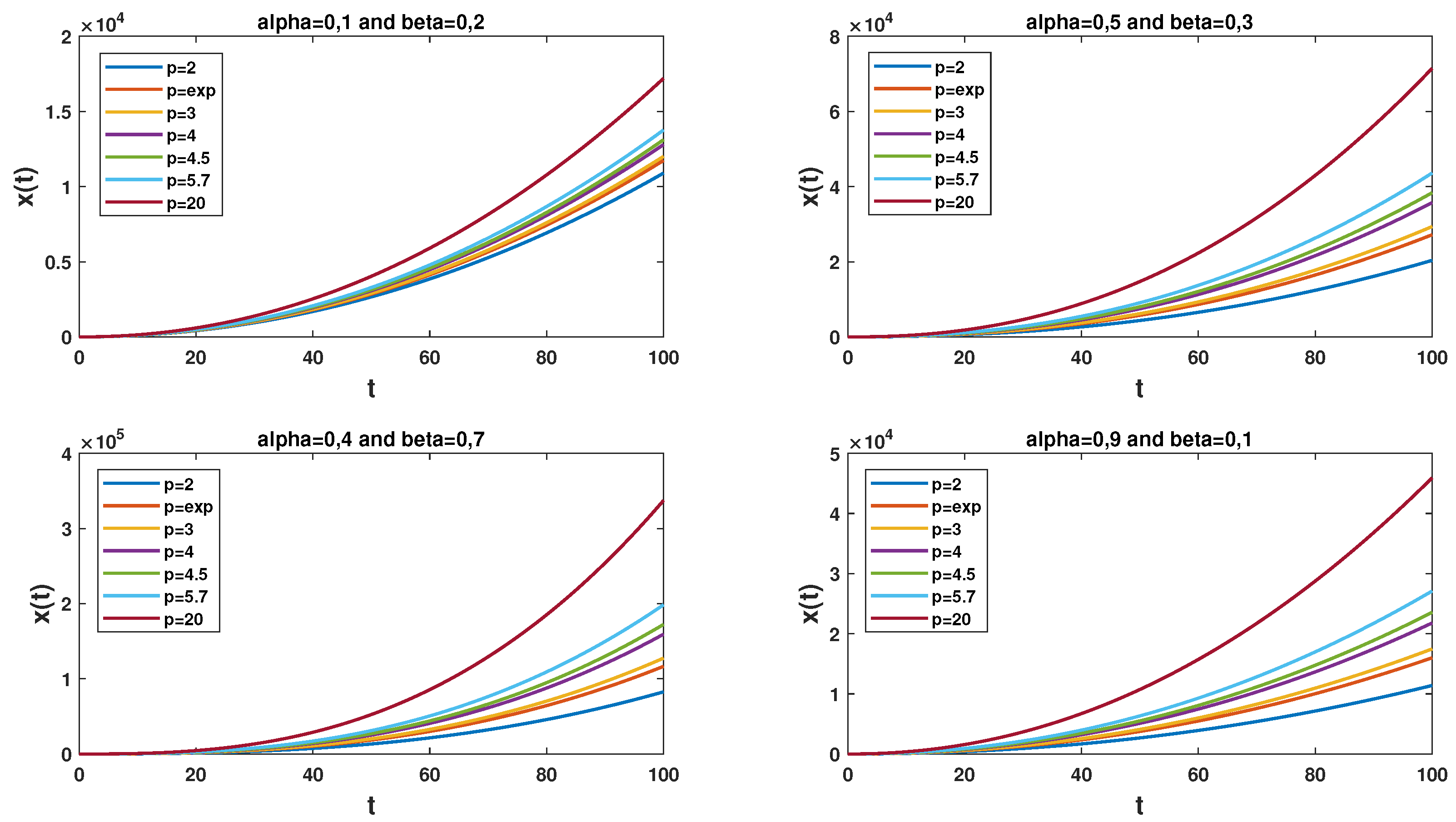
5. Examples of Power Fractional Differential Equations

In this section, we treat two examples of power fractional differential equations (PFDEs). Our first example considers a non-autonomous PFDE in the Riemann–Liouville sense.

Example 1.

Consider the following non-autonomous PFDE on $[0,100]$:

$${}^{p_{RL}}{D}_{0,t,\frac{1}{t^2}}^{\alpha ,\beta ,p}x\left(t\right)=t^2,x\left(0\right)=0.$$

(18)

Using Theorem 4, we obtain that

$$\begin{array}{cc}\hfill x\left(t\right)& =\varphi \left(\alpha \right)t^2+lnp·\psi \left(\alpha \right)·{}^p{I}_{0,t,\frac{1}{t^2}}^{\alpha ,\beta ,p}{t}^2\hfill \\ \hfill & =\varphi \left(\alpha \right)t^2+lnp·\psi \left(\alpha \right){\displaystyle \frac{t^{\beta +2}}{\Gamma (\beta +1)}}.\hfill \end{array}$$

(19)

The action of the parameter p on the obtained solution is shown in Figure 1.

We now consider an autonomous PFDE in the Caputo sense.

Example 2.

Consider the following autonomous PFDE:

$${}^{p_C}{D}_{0,t,w}^{\alpha ,\beta ,p}x\left(t\right)=Ax\left(t\right)+B,x\left(0\right)=x_0.$$

(20)

The action of the Laplace transform on both sides of Equation (20) yields:

$$\mathcal{L}\left\{w\left(t\right){}^{p_C}{D}_{0,t,w}^{\alpha ,\beta ,p}x\left(t\right)\right\}\left(s\right)=A\mathcal{L}\left\{w\left(t\right)x\left(t\right)\right\}\left(s\right)+B\mathcal{L}\left\{w\left(t\right)\right\}\left(s\right).$$

Using Lemma 1, we obtain that

$$\begin{array}{ccc}\hfill \mathcal{L}\left\{w\right(t\left)x\right(t\left)\right\}\left(s\right)& =& \frac{B(1-\alpha )s^{\beta }+\alpha Alnp}{[N\left(\alpha \right)-(1-\alpha )A]s^{\beta }-\alpha Alnp}\mathcal{L}\left\{w\left(t\right)\right\}\left(s\right)\hfill \\ & & +\frac{N\left(\alpha \right)w\left(0\right)x\left(0\right)s^{\beta -1}}{[N\left(\alpha \right)-(1-\alpha )A]s^{\beta }-\alpha Alnp}\hfill \\ & =& \frac{N\left(\alpha \right)w\left(0\right)x\left(0\right)}{\left[N\right(\alpha )-(1-\alpha \left)A\right]}\frac{s^{\beta -1}}{s^{\beta }-\frac{\alpha Alnp}{\left[N\right(\alpha )-(1-\alpha \left)A\right]}}\hfill \\ & & +\frac{B(1-\alpha )}{\left[N\right(\alpha )-(1-\alpha \left)A\right]}\frac{s^{\beta -1}}{s^{\beta }-\frac{\alpha Alnp}{\left[N\right(\alpha )-(1-\alpha \left)A\right]}}s\mathcal{L}\left\{w\left(t\right)\right\}\left(s\right)\hfill \\ & & +\frac{\alpha Blnp}{\left[N\right(\alpha )-(1-\alpha \left)A\right]}\frac{1}{s^{\beta }-\frac{\alpha Alnp}{\left[N\right(\alpha )-(1-\alpha \left)A\right]}}\mathcal{L}\left\{w\left(t\right)\right\}\left(s\right)\hfill \\ & =& \frac{N\left(\alpha \right)w\left(0\right)x_0}{\left[N\right(\alpha )-(1-\alpha \left)A\right]}\mathcal{L}\left\{{}^p{E}_{\beta ,1}\left(\frac{\alpha A}{\left[N\right(\alpha )-(1-\alpha \left)A\right]}{t}^{\beta }\right)\right\}\left(s\right)\hfill \\ & & +\frac{(1-\alpha )B}{\left[N\right(\alpha )-(1-\alpha \left)A\right]}\mathcal{L}\left\{{}^p{E}_{\beta ,1}\left(\frac{\alpha A}{\left[N\right(\alpha )-(1-\alpha \left)A\right]}{t}^{\beta }\right)\right\}\left(s\right)\hfill \\ & & \times \left(\mathcal{L}\left\{w^{\prime }\left(t\right)\right\}\left(s\right)+w\left(0\right)\right)\hfill \\ & & +\frac{B}{A}\mathcal{L}\left\{\frac{d}{dt}{}^p{E}_{\beta ,1}\left(\frac{\alpha A}{\left[N\right(\alpha )-(1-\alpha \left)A\right]}{t}^{\beta }\right)\right\}\left(s\right)\mathcal{L}\left\{w\left(t\right)\right\}\left(s\right).\hfill \end{array}$$

The effect of the inverse Laplace transform operator yields

$$\begin{array}{ccc}\hfill w\left(t\right)x\left(t\right)& =& \frac{N\left(\alpha \right)w\left(0\right)x_0}{\left[N\right(\alpha )-(1-\alpha \left)A\right]}{}^p{E}_{\beta ,1}\left(\frac{\alpha A}{\left[N\right(\alpha )-(1-\alpha \left)A\right]}{t}^{\beta }\right)\hfill \\ & & +\frac{(1-\alpha )B}{\left[N\right(\alpha )-(1-\alpha \left)A\right]}{}^p{E}_{\beta ,1}\left(\frac{\alpha A}{\left[N\right(\alpha )-(1-\alpha \left)A\right]}{t}^{\beta }\right)\ast w^{\prime }\left(t\right)\hfill \\ & & +\frac{(1-\alpha )Bw\left(0\right)}{\left[N\right(\alpha )-(1-\alpha \left)A\right]}{}^p{E}_{\beta ,1}\left(\frac{\alpha A}{\left[N\right(\alpha )-(1-\alpha \left)A\right]}{t}^{\beta }\right)\hfill \\ & & +\frac{B}{A}\left(\frac{d}{dt}{}^p{E}_{\beta ,1}\left(\frac{\alpha A}{\left[N\right(\alpha )-(1-\alpha \left)A\right]}{t}^{\beta }\right)\right)\ast w\left(t\right).\hfill \end{array}$$

Applying the integration by parts formula on$\left(\frac{d}{dt}{}^p{E}_{\beta ,1}\left(\frac{\alpha A}{\left[N\right(\alpha )-(1-\alpha \left)A\right]}{t}^{\beta }\right)\right)\ast w\left(t\right)$, we can state that the solution to problem (20) is given by

$$\begin{array}{ccc}\hfill x\left(t\right)& =& \frac{-B}{A}+\frac{N\left(\alpha \right)w\left(0\right)}{\left[N\right(\alpha )-(1-\alpha \left)A\right]w\left(t\right)}\left(x_0+\frac{B}{A}\right){}^p{E}_{\beta ,1}\left(\frac{\alpha A}{\left[N\right(\alpha )-(1-\alpha \left)A\right]}{t}^{\beta }\right)\hfill \\ & & -\frac{AN\left(\alpha \right)}{A\left[N\right(\alpha )-(1-\alpha \left)A\right]w\left(t\right)}{}^p{E}_{\beta ,1}\left(\frac{\alpha A}{\left[N\right(\alpha )-(1-\alpha \left)A\right]}{t}^{\beta }\right)\ast w^{\prime }\left(t\right).\hfill \end{array}$$

6. Conclusions

In this paper, some new mathematical concepts, enabling the introduction of a new extended fractional calculus, are provided. The new approach allows choice of the most appropriate notion of differentiation to suitably describe real dynamic phenomena under study, describing the observed trajectories and correctly predicting future behaviors. More precisely, we introduce the “power Mittag–Leffler function” ${}^p{E}_{\alpha ,\beta }(·)$ that extends several important functions: the Mittag–Leffler function ${}^e{E}_{\alpha ,1}(·)$, first introduced by Mittag–Leffler in [12]; the function ${}^e{E}_{\alpha ,\beta }(·)$ of Wiman [13]; and those introduced by Prabhakar [14] and Salim [16]. With the help of the new power Mittag–Leffler function, we then introduce the new power fractional derivatives ${}^{p_C}{D}_{a,t,w}^{\alpha ,\beta ,p}(·)$ and ${}^{p_{RL}}{D}_{a,t,w}^{\alpha ,\beta ,p}(·)$, which generalize those available in the literature, namely the Caputo–Fabrizio [3], Atangana–Baleanu [4], weighted Atangana–Baleanu [5], and weighted generalized fractional derivatives [6]. Moreover, an appropriate power fractional integral operator (PFIO) ${}^p{I}_{a,t,w}^{\alpha ,\beta ,p}(·)$ is introduced, which is an important tool for the solution of power fractional differential equations (PFDEs). As examples, we investigated two PFDEs. The first is a non-autonomous PFDE: using our PFIO, we compute its solution and illustrate, numerically, the impact of the parameter p on the solution. The second example considered is an autonomous PFDE and its solution is obtained using the Laplace transform operator.

Here, we have only introduced the power fractional calculus and provided the most fundamental results with some applications to power fractional differential equations. In future work, several investigations may be designed to develop the new fractional calculus, which will enable the setting up of numerous applications on many parallel domains, e.g., in the fractional neural networks framework, analogously to what is done in [20,21,22].

References

1. Ding, L.; Luo, Y.; Lin, Y.; Huang, Y. Revisiting the relations between Hurst exponent and fractional differencing parameter for long memory. Physica A 2021, 566, 125603. [Google Scholar] [CrossRef]
2. Kee, C.Y.; Chua, C.; Zubair, M.; Ang, L.K. Fractional modeling of urban growth with memory effects. Chaos 2022, 32, 083127. [Google Scholar] [CrossRef] [PubMed]
3. Caputo, M.; Fabrizio, M. A new definition of fractional derivative without singular kernel. Progr. Fract. Differ. Appl. 2015, 1, 73–85. [Google Scholar]
4. Atangana, A.; Baleanu, D. New fractional derivatives with non-local and non-singular kernel: Theory and application to heat transfer model. Therm. Sci. 2016, 20, 763–769. [Google Scholar] [CrossRef] [Green Version]
5. Al-Refai, M. On weighted Atangana-Baleanu fractional operators. Adv. Differ. Equ. 2020, 2020, 3. [Google Scholar] [CrossRef] [Green Version]
6. Hattaf, K. A new generalized definition of fractional derivative with non-singular kernel. Computation 2020, 8, 49. [Google Scholar] [CrossRef]
7. Zine, H.; Torres, D.F.M. A stochastic fractional calculus with applications to variational principles. Fractal Fract. 2020, 4, 38. [Google Scholar] [CrossRef]
8. Boukhouima, A.; Hattaf, K.; Lotfi, E.M.; Mahrouf, M.; Torres, D.F.M.; Yousfi, N. Lyapunov functions for fractional-order systems in biology: Methods and applications. Chaos Solitons Fractals 2020, 140, 110224. [Google Scholar] [CrossRef]
9. Zine, H.; Lotfi, E.M.; Torres, D.F.M.; Yousfi, N. Weighted generalized fractional integration by parts and the Euler-Lagrange equation. Axioms 2022, 11, 178. [Google Scholar] [CrossRef]
10. Zine, H.; Lotfi, E.M.; Torres, D.F.M.; Yousfi, N. Taylor’s formula for generalized weighted fractional derivatives with nonsingular kernels. Axioms 2022, 11, 231. [Google Scholar] [CrossRef]
11. Boukhouima, A.; Zine, H.; Lotfi, E.M.; Mahrouf, M.; Torres, D.F.M.; Yousfi, N. Lyapunov functions and stability analysis of fractional-order systems. In Mathematical Analysis of Infectious Diseases; Elsevier: London, UK, 2022; Chapter 8; pp. 125–136. [Google Scholar] [CrossRef]
12. Mittag-Leffler, G.M. Sur la nouvelle fonction Eα(x). C. R. L’Acad. Sci. Paris 1903, 137, 554–558. [Google Scholar]
13. Wiman, A. Über den Fundamentalsatz in der Teorie der Funktionen Ea(x). Acta Math. 1905, 29, 191–201. [Google Scholar] [CrossRef]
14. Prabhakar, T.R. A singular integral equation with a generalized Mittag Leffler function in the kernel. Yokohama Math. J. 1971, 19, 7–15. [Google Scholar]
15. Shukla, A.K.; Prajapati, J.C. On a generalization of Mittag-Leffler function and its properties. J. Math. Anal. Appl. 2007, 336, 797–811. [Google Scholar] [CrossRef] [Green Version]
16. Salim, T.O. Some properties relating to the generalized Mittag-Leffler function. Adv. Appl. Math. Anal. 2009, 4, 21–30. [Google Scholar]
17. Salim, T.O.; Faraj, A.W. A generalization of Mittag-Leffler function and integral operator associated with fractional calculus. J. Fract. Calc. Appl. 2012, 3, 1–13. [Google Scholar]
18. Khan, M.A.; Ahmed, S. On some properties of the generalized Mittag-Leffler function. SpringerPlus 2013, 2, 337. [Google Scholar] [CrossRef] [Green Version]
19. Khan, N.; Ghayasuddin, M.; Shadab, Ṁ. Some generating relations of extended Mittag-Leffler functions. Kyungpook Math. J. 2019, 59, 325–333. [Google Scholar] [CrossRef]
20. Xiao, J.; Guo, X.; Li, Y.; Wen, S.; Shi, K.; Tang, Y. Extended analysis on the global Mittag-Leffler synchronization problem for fractional-order octonion-valued BAM neural networks. Neural Netw. 2022, 154, 491–507. [Google Scholar] [CrossRef]
21. Xiao, J.; Zhong, S.; Wen, S. Unified analysis on the global dissipativity and stability of fractional-order multidimension-valued memristive neural networks with time delay. IEEE Trans. Neural Netw. Learn. Syst. 2021. [Google Scholar] [CrossRef]
22. Xiao, J.; Li, Y. Novel synchronization conditions for the unified system of multi-dimension-valued neural networks. Mathematics 2022, 10, 3031. [Google Scholar] [CrossRef]
Figure 1. Impact of the power parameter p on the solution x ( t ) (19) of problem (18) of Example 1 with different values of orders α and β .
Mathematics 10 03594 g001
Publisher’s Note: MDPI stays neutral with regard to jurisdictional claims in published maps and institutional affiliations.