Two Interval Upper-Bound Q-Function Approximations with Applications

Abstract

The Gaussian Q-function has considerable applications in numerous areas of science and engineering. However, the fact that a closed-form expression for this function does not exist encourages finding approximations or bounds of the Q-function. In this paper, we determine analytically two novel interval upper bound Q-function approximations and show that they could be used efficiently not only for the symbol error probability (SEP) estimation of transmission over Nakagami-m fading channels, but also for the average symbol error probability (ASEP) evaluation for two modulation formats. Specifically, we determine analytically the composition of the upper bound Q-function approximations specified at disjoint intervals of the input argument values so as to provide the highest accuracy within the intervals, by utilizing the selected one of two upper bound Q-function approximations. We show that a further increase of the accuracy, achieved in the case with two upper-bound approximations composing the interval approximation, can be obtained by forming a composite interval approximation of the Q-function that assumes another extra interval and by specifying the third form for the upper-bound Q-function approximation. The proposed analytical approach can be considered universal and widely applicable. The results presented in the paper indicate that the proposed Q-function approximations outperform in terms of accuracy other well-known approximations carefully chosen for comparison purposes. This approximation can be used in numerous theoretical communication problems based on the Q-function calculation. In this paper, we apply it to estimate the average bit error rate (ABER), when the transmission in a Nakagami-m fading channel is observed for the assumed binary phase-shift keying (BPSK) and differentially encoded quadrature phase-shift keying (DE-QPSK) modulation formats, as well as to design scalar quantization with equiprobable cells for variables from a Gaussian source.

1. Introduction

The growing need for the mathematical characterization of complex phenomena in wireless transmission has occurred due to the recent rapid development of various wireless communication system services [1,2]. Determining the performance of the wireless communication systems and observing how this performance depends on key transmission system parameter values are of importance for estimating the behavior of digital communication systems for a wide range of applied modulation types, detection types, and channel models (see for instance [1,2,3,4,5]). Signal transmission in a wireless medium is accompanied by various phenomena, among which the most important one is multipath fading. In the literature, various mathematical models of this fading phenomenon have been presented. As shown in [2], the Nakagami-m fading model provides the best fit for collected data in indoor and outdoor wireless environments. The average symbol error probability (ASEP) of a wireless communication system best quantifies the reliability or integrity of a received signal [1]. To analytically determine the ASEP for an assumed modulation format, it is necessary to average the expression for the conditional symbol error probability (SEP) over the probability density function (PDF) of the fading channel amplitude [1]. However, in most of the observed cases, the averaging is not straightforward because the averaging integral includes the Gaussian Q-function or directly related special functions: error function, erf(x), and/or complementary error function erfc(x) [1,2,3,4,5]. Thus, the motivation of our research was to examine the possibility of deriving a novel, simple, highly accurate Q-function approximation, which could be used efficiently not only for the SEP estimation of transmission over Nakagami-m fading channels, but also for the ASEP evaluation. Although this problem has been extensively reported in the literature [1,2,3,4,5,6,7,8,9,10,11,12,13,14,15,16,17,18,19,20], the need for simpler and more accurate Q-function approximations still exists due to the continuous development of various wireless services. In regards to some of our previous research works [4,21,22,23], herein, tighter bounds are observed in order to obtain better and more accurate results.

The main goal of this paper was to simplify the selection of the approximation of the Q-function proposed in [6], where four different approximations were shown to approximate the Q-function for each argument value, which made such a choice cumbersome. Toward this goal, we first select two of these four approximations of the Q-function and determine analytically which of the two selected upper-bound approximations of the Q-function provides the best result in terms of accuracy for the widest interval of argument values. In other words, we determine the composition of the upper-bound Q-function approximations specified on the two disjoint intervals of input argument values so as to provide the highest accuracy within each of them. We show that a further increase of the accuracy can be obtained by forming a composite approximation of the Q-function that assumes another extra interval for the highest argument values and by specifying an additional form for the third upper-bound Q-function approximation.

The rest of this paper is organized as follows: Section 2 describes the main motivation of this paper and gives a brief overview of the previous work in the field. In Section 3, the novel interval upper-bound Q-function approximations are specified. Section 4 provides the accuracy analysis of the novel interval upper-bound Q-function approximations and the approximations of the Q-function listed in Section 2. Section 5 demonstrates the applicability of the proposed Q-function approximations in the ASEP evaluation over Nakagami-m fading channels when BPSK and DE-QPSK modulation formats are assumed. In Section 6, we explore some new benefits of Q-function approximations, such as applications in designing quantization with equiprobable cells for Gaussian sources. Finally, Section 7 concludes on our research results.

As already stated, in numerous areas of science and engineering, we encounter the Gaussian Q-function. This paper also aims to explore the benefits of approximating the Q-function by a closed form expression when quantization issues are in question. In particular, we consider the quantization of variables from a Gaussian source, where the probability that the variable belongs to a particular cell is the difference of two Q-functions. With the goal to achieve equiprobable quantization cells, in [24], a quantization noise was injected. Unlike [24], in this paper, the equiprobable quantization cells and quantizer design are specified in a different way. To design the quantizer for the assumed Gaussian source having equiprobable quantization cells, the system of integral equations with arguments of Q-functions as unknown variables has to be solved. With the application of the composite upper-bound approximation proposed in this paper, we manage to avoid solving the systems of integral equations, which makes our proposal useful.

In brief, the main contributions of this paper are:

-

We propose an analytical approach for determining the composition of upper-bound Q-function approximations specified on disjoint intervals of input argument values so as to provide the highest accuracy within the intervals by utilizing the disposable upper-bound approximations of the Q-function;

-

We determine particular analytical forms of two such compositions, named interval upper-bound Q-function approximations;

-

We demonstrate that a further increase of the accuracy, achieved in the case with two upper-bound approximations composing the interval approximation, can be obtained by forming a composite interval approximation of the Q-function that assumes another extra interval and by specifying the third form for the upper-bound Q-function approximation;

-

We show that in the whole domain of the function argument, our novel interval upper-bound Q-function approximations provide noticeable improvements in terms of the accuracy in comparison with Q-function approximations of similar analytical forms from the literature selected for comparison purposes;

-

We analyze the versatility of our proposal in determining the performance (ABER), when the transmission in Nakagami-m fading channel is observed for the assumed BPSK and DE-QPSK modulation formats and provide an additional justification of the benefits of using the proposed composite improved interval approximation of the Q-function (our second upper-bound composite interval approximation of the Q-function) in designing wireless communication systems for an accurate estimation of the expected QoS (quality of service);

-

We demonstrate the usefulness of our proposal in issues occurring in designing scalar quantizers for the Gaussian source.

In

Table 1. Table of important symbols used throughout the paper, in order of appearance.

Symbol	Brief Description
$Q\left(x\right)$	Gaussian Q-function
$erfc$	Complementary error function
$Q^{\left[11\right]}$	Jang’s Q-function approximation
$Q^{\left[12\right]}$	Q-function approximation by Chiani et al.
$Q^{\left[13\right]}$	Abreu’s Q-function approximation
$Q^{\left[14\right]}$	Q-function approximation by Borjesson et al.
${Q_1}^{\left[7\right]}$ and ${Q_1}^{\left[7\right]}$	Q-function approximations by Gasull and Utzet
$Q^{com\_1}$ and $Q^{com\_2}$	Q-function approximations by authors
$P_b$	Conditional SEP over the Nakagami-m fading channel amplitude for the assumed modulation format
$E_b$ and $N_0$	Average bit energy and the one-sided noise power spectral density, respectively,
f${}_x$(x)	PDF of the Nakagami-m fading channel amplitude
$\mathrm{\Omega }$	Average signal power
m	Inverse normalized variance of x
$\Gamma$(m)	Special gamma function
$f_{\gamma }\left(\gamma \right)$	Nakagami-m PDF of the signal-to-noise ratio (SNR) per symbol
$\overline{\gamma }$	Average SNR per symbol
$\gamma$	Relation between received carrier amplitude under fading influence x, its mean squared value $\mathrm{\Omega }$, and the instantaneous signal-to-noise power ratio (SNR) per symbol.

we present the symbols used in paper and their brief description.

2. Related Work and Motivation

The main motivation of numerous research studies [7,8,9,10,11,12,13,14,15], including the one presented in this paper, is to solve the problem of deriving closed-form expressions for the SEP evaluation for signals with a Gaussian probability density function (PDF). In particular, the problem reduces to providing a closed-form formula that approximates the Q-function, given by [25,26]:

$$Q\left(x\right)=\frac{1}{\sqrt{2\pi }}{\int }_x^{\infty }exp\left\{-\frac{t^2}{2}\right\}dt.$$

(1)

The Gaussian Q-function can be expressed in terms of the complementary error function:

$$Q\left(x\right)\stackrel{\Delta }{=}\frac{1}{2}\mathrm{erfc}\left(\frac{x}{\sqrt{2}}\right),$$

(2)

given by [18,19]:

$$erfc\left(x\right)=\frac{2}{\sqrt{\pi }}{\int }_x^{\infty }exp\left\{-t^2\right\}dt.$$

(3)

In [11], Jang proposed a simple upper-bound approximation of the Gaussian Q-function for x ≥ 0, in the form

$$Q^{\left[11\right]}\left(x\right)=\frac{1}{\sqrt{2\pi }}\frac{1}{x}\left(1-exp\left\{-\sqrt{\frac{\pi }{2}}x\right\}\right)exp\left\{-\frac{x^2}{2}\right\}.$$

(4)

Chiani derived analytically an even simpler upper-bound approximation of the Q-function in the form of the sum of two exponential functions [12]:

$$Q^{\left[12\right]}\left(x\right)=\frac{1}{12}exp\left\{-\frac{x^2}{2}\right\}+\frac{1}{4}exp\left\{-\frac{2x^2}{3}\right\},$$

(5)

which is the upper-bound approximation of the Q-function for x > 0.5.

Although it has been highlighted in [11,16,17,27] that the bounds for the Q-function could have complex mathematical forms, nevertheless, an upper-bound approximation on the Q-function that was very accurate for small argument values and less accurate for higher argument values was proposed in ([13] Equation (12)) as:

$$Q^{\left[13\right]}\left(x\right)=\frac{1}{50}exp\left\{-x^2\right\}+\frac{1}{2\left(x+1\right)}exp\left\{-\frac{x^2}{2}\right\}.$$

(6)

Another useful and practical Q-function approximation that we took into consideration in this paper was given in ([14], Equation (9)):

$$Q^{\left[14\right]}\left(x\right)=\frac{1}{\sqrt{2\pi }}\frac{1}{\sqrt{x^2+1}}exp\left\{-\frac{x^2}{2}\right\}.$$

(7)

As already mentioned, we chose two upper-bound approximations of the Q-function from [7]:

$$Q_1^{\left[7\right]}\left(x\right)=\frac{1}{\sqrt{2\pi }}\frac{\pi }{2x+\sqrt{{\left(\pi -2\right)}^2{x}^2+2\pi }}exp\left\{-\frac{x^2}{2}\right\},$$

(8)

and

$$Q_2^{\left[7\right]}\left(x\right)=\frac{1}{\sqrt{2\pi }}\frac{4}{3x+\sqrt{x^2+8}}exp\left\{-\frac{x^2}{2}\right\},$$

(9)

and analytically determined the disjoint intervals of the value of the argument x in which it was convenient to apply these approximations so that the accuracy due to the approximation of the Q-function by the considered upper-bound approximations was the highest possible.

3. Two Novel Interval Upper-Bound Q-Function Approximations

Lemma 1.

There exists a unique $x_1\in [0,+\infty )$ such that $Q_1^{\left[7\right]}\left(x\right)\le Q_2^{\left[7\right]}\left(x\right)$ if and only if $x\le x_1$ ($x\in [0,+\infty ]$).

Proof. 

Inequality $Q_1^{\left[7\right]}\left(x\right)\le Q_2^{\left[7\right]}\left(x\right)$ is equivalent to

$$(3\pi -8)x+\pi \sqrt{x^2+8}\le 4\sqrt{{(\pi -2)}^2{x}^2+2\pi }.$$

Squaring both sides and regrouping factors yields

$$x\sqrt{x^2+8}\le x^2+\frac{4(4-\pi )}{3\pi -8}.$$

Again, squaring both sides of the inequality and rearranging terms gives

$$x\le x_1:=\frac{4-\pi }{\sqrt{2(\pi -3)(3\pi -8)}}$$

That finishes the proof of the lemma. □

Let us define the following composition of the Q-function approximations, Q${}^{com\_1}$(x), such that $Q^{com\_1}\left(x\right)=Q_1^{\left[7\right]}\left(x\right)$ for $x\in [0,x_1)$ and $Q^{com\_1}\left(x\right)=Q_2^{\left[7\right]}\left(x\right)$ for $x\in [x_1,+\infty )$. In other words, let

$$Q^{\mathrm{com}\_1}\left(x\right)=\left\{\begin{array}{c}\frac{1}{\sqrt{2\pi }}\frac{\pi }{2x+\sqrt{{\left(\pi -2\right)}^2{x}^2+2\pi }}exp\left\{-\frac{x^2}{2}\right\},0\le x<x_1\hfill \\ \frac{1}{\sqrt{2\pi }}\frac{4}{3x+\sqrt{x^2+8}}exp\left\{-\frac{x^2}{2}\right\},x\ge x_1\hfill \end{array}\right..$$

(10)

According to the previous lemma, function $Q^{com\_1}\left(x\right)$ is continuous and $Q^{com\_1}\left(x\right)=min\{Q_1^{\left[7\right]}\left(x\right),Q_2^{\left[7\right]}\left(x\right)\}$ for every $x\in [0,+\infty )$. This means that $Q^{com\_1}\left(x\right)$ is a tighter upper bound of the Q-function than both $Q_1^{\left[7\right]}\left(x\right)$ and $Q_2^{\left[7\right]}\left(x\right)$. The fact that the value for $x_1$ can be obtained analytically widens the possible applications of $Q^{com\_1}\left(x\right)$ in both analytical and numerical computations.

Lemma 2.

There exist values $t_1\in (0,x_1)$ and $t_2\in [x_1,+\infty )$ such that $Q^{\left[13\right]}\left(t_i\right)=Q^{com\_1}\left(t_i\right)$$(i=1,2)$.

Proof. 

One can verify by direct computation that $Q^{\left[13\right]}\left(0\right)>Q^{com\_1}\left(0\right)=Q_1^{\left[7\right]}\left(0\right)$, $Q^{\left[13\right]}\left(x_1\right)<Q^{com\_1}\left(x_1\right)$ and $Q^{\left[13\right]}\left(2\right)>Q^{com\_1}\left(2\right)=Q_2^{\left[7\right]}\left(2\right)$. According to that, equations $Q^{\left[13\right]}\left(x\right)-Q_1^{\left[7\right]}\left(x\right)=0$ and $Q^{\left[13\right]}\left(x\right)-Q_2^{\left[7\right]}\left(x\right)=0$ have at least one root on intervals $(0,x_1)$ and $(x_1,+\infty )$, respectively. □

Note that numerical evaluations suggest that values $t_1$ and $t_2$ from the previous lemma are unique and approximately equal to $t_1\approx 0.499286$ and $t_2\approx 1.72519$. Therefore, one can conclude that $Q^{\left[13\right]}\left(x\right)\le Q^{com\_1}\left(x\right)$ if and only if $x\in [t_1,t_2]$. Using that fact, we can define the following composite upper bound for the Q-function:

$$Q^{\mathrm{com}\_2}\left(x\right)=\left\{\begin{array}{c}\frac{1}{\sqrt{2\pi }}\frac{\pi }{2x+\sqrt{{\left(\pi -2\right)}^2{x}^2+2\pi }}exp\left\{-\frac{x^2}{2}\right\},0\le x<t_1\hfill \\ \frac{1}{50}exp\left\{-x^2\right\}+\frac{1}{2\left(x+1\right)}exp\left\{-\frac{x^2}{2}\right\},t_1\le x<t_2\hfill \\ \frac{1}{\sqrt{2\pi }}\frac{4}{3x+\sqrt{x^2+8}}exp\left\{-\frac{x^2}{2}\right\},x\ge t_2\hfill \end{array}\right..$$

(11)

Although the approximation of the Q-function by Q${}^{com\_1}$(x) is simpler, if a higher accuracy is demanded, then a better choice is the approximation of the Q-function with Q${}^{com\_2}$(x).

4. Accuracy Analysis of the Q-Function Approximations

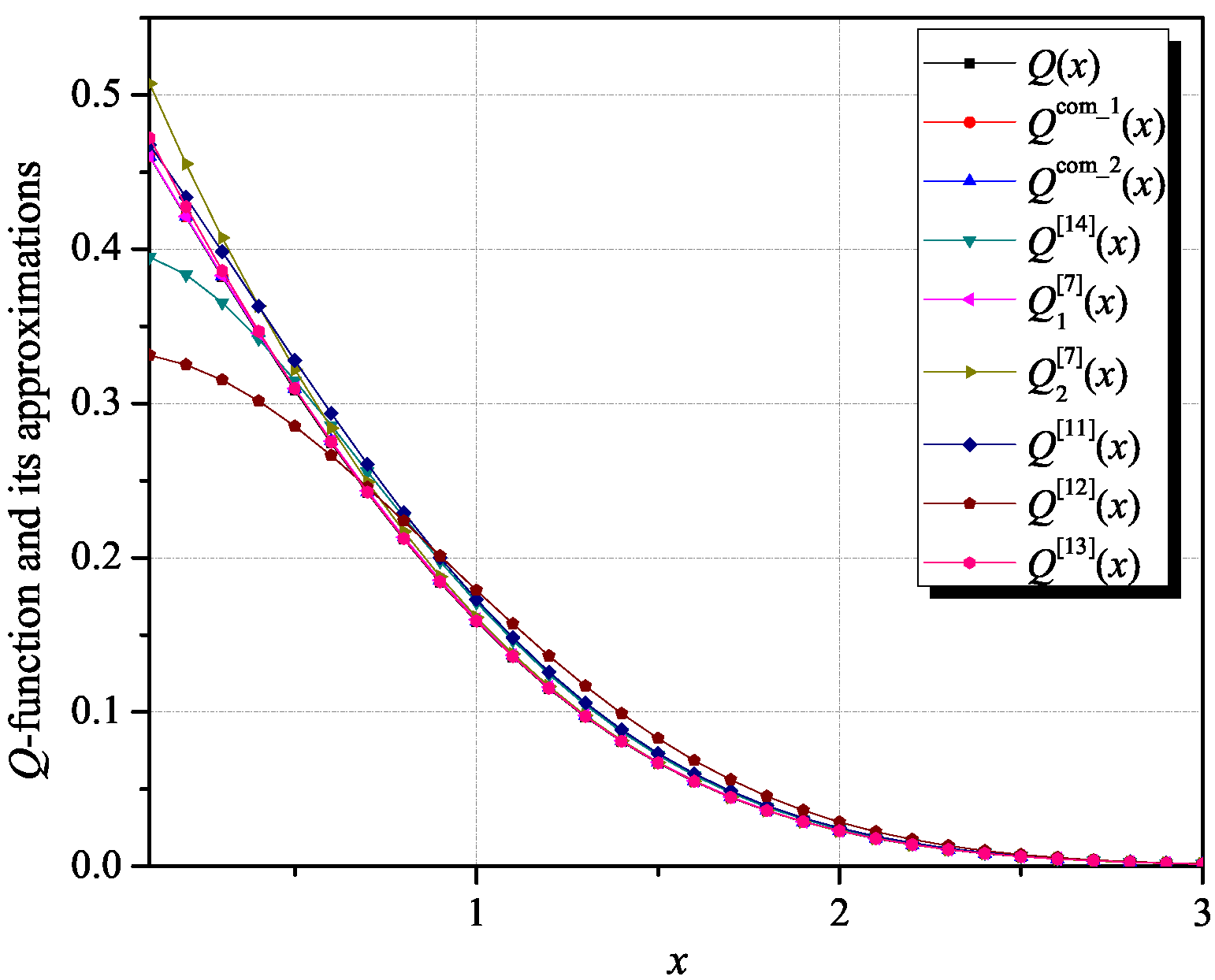
Figure 1 presents the comparison of the Q-function and its approximations, where along with the selected approximations of the Q-function from the literature [7,11,12,13,14], two novel approximations of the Q-function are presented as well. Although it is not very visible from Figure 1, we show below that the proposed composite approximation of the Q-function, specified for x${}_1$ = 1.3514, that is, for intervals determined from Lemma1 as [0, 1.3514) and [1.3514, ∞), outperforms in terms of accuracy the Q-function approximations used for comparison purposes. The results of approximating the Q-function for different values of x are presented in

Table 2. Comparison of several Q-function approximations for discrete values of argument x.

	x = 0.1	x = 0.3	x = 0.5	x = 0.7	x = 1	x = 5	x = 10	x = 15	x = 20
Q(x)	0.46017	0.38209	0.30854	0.24196	0.15866	$2.8665\times {10}^{-7}$	$7.6199\times {10}^{-7}$	$3.6710\times {10}^{-51}$	$2.7536\times {10}^{-89}$
Q${}^{\left[14\right]}$(x)	0.39498	0.36530	0.31490	0.25581	0.17110	$2.9157\times {10}^{-7}$	$7.6564\times {10}^{-24}$	$3.6790\times {10}^{-51}$	$2.7570\times {10}^{-89}$
Q${}_1^{\left[7\right]}\left(\mathit{x}\right)$	0.46030	0.38281	0.30975	0.24336	0.15989	$2.8771\times {10}^{-7}$	$7.6286\times {10}^{-24}$	$3.673\times {10}^{-24}$	$2.755\times {10}^{-89}$
Q${}_2^{\left[7\right]}$(x)	0.50725	0.40743	0.3221	0.24912	0.16131	$2.8667\times {10}^{-7}$	$7.6199\times {10}^{-24}$	$3.671\times {10}^{-51}$	$2.7536\times {10}^{-89}$
Q${}^{\left[11\right]}$(x)	0.46759	0.39842	0.32786	0.26056	0.17287	$2.9678\times {10}^{-7}$	$7.6946\times {10}^{-24}$	$3.6871\times {10}^{-51}$	$2.7605\times {10}^{-89}$
Q${}^{\left[12\right]}$(x)	0.33126	0.31511	0.28516	0.24556	0.17890	$3.2500\times {10}^{-7}$	$1.6073\times {10}^{-23}$	$1.1553\times {10}^{-50}$	$1.1532\times {10}^{-88}$
Q${}^{\left[13\right]}$(x)	0.4721	0.38597	0.30974	0.24246	0.15899	$3.1055\times {10}^{-7}$	$8.767\times {10}^{-24}$	$4.3323\times {10}^{-51}$	$3.2949\times {10}^{-89}$
Q${}^{\mathit{c}\mathit{o}\mathit{m}\_1}$(x)	0.46030	0.38281	0.30975	0.24336	0.15989	$2.8771\times {10}^{-7}$	$7.6286\times {10}^{-24}$	$3.673\times {10}^{-51}$	$2.7550\times {10}^{-89}$
Q${}^{\mathit{c}\mathit{o}\mathit{m}\_2}$(x)	0.46029	0.38279	0.30973	0.24246	0.15899	$2.8667\times {10}^{-7}$	$7.6199\times {10}^{-24}$	$3.671\times {10}^{-51}$	$2.7536\times {10}^{-89}$

.

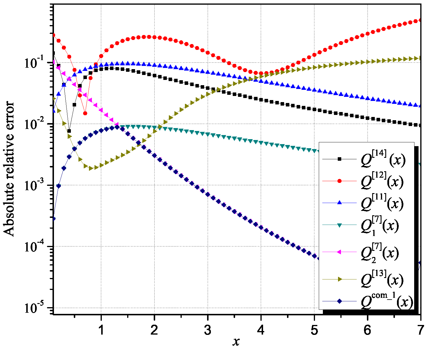
Figure 2 presents the comparison of the absolute relative error calculated for the proposed first interval upper-bound approximation of the Q-function and selected ones from the literature [7,11,12,13,14]. As visible from Figure 2, the approximation specified by Lemma 1 for x${}_1$ = 1.3514 has a minimal absolute relative error and is more accurate than other considered Q-function approximations in almost the entire observed range of argument values.

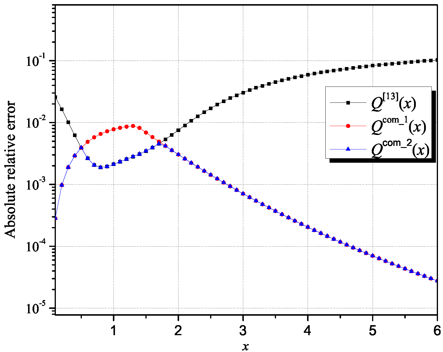
Figure 3 presents the comparison of the absolute relative errors of the two novel interval upper-bound approximations of the Q-function with the one from [13]. Although with the first interval upper-bound approximation of the Q-function, Q${}^{com\_1}$(x), a better approximation (lower values of the absolute relative error) has been obtained in a wide range of argument values compared to the Q-function approximation from [13], there is still an interval in which better results in terms of accuracy can be obtained by using a slightly more complex second interval upper-bound approximation of the Q-function, Q${}^{com\_2}$(x). In other words, we ascertained that an additional improvement of the accuracy in the whole range of argument values could be obtained by prudently forming the second composite interval upper-bound approximation of the Q-function specified by Lemma 2.

5. Application to Fading Channels Performance Analysis

Let us now exploit the advantages of the application of the proposed Q-function approximations in the ASEP evaluation over Nakagami-m fading channels when a BPSK modulation is assumed. To numerically evaluate the ASEP, we need to average the expression for the conditional SEP over the Nakagami-m fading channel amplitude for the assumed modulation format, i.e., to evaluate the following expression:

$$P_b={\int }_0^{\infty }Q\left(\sqrt{\frac{2E_b}{N_0}}x\right)f_x\left(x\right)dx,$$

(12)

where f${}_x$(x) is the PDF of the Nakagami-m fading channel amplitude. E${}_b$ and N${}_0$ denote the average bit energy and the one-sided noise power spectral density, respectively.

The Nakagami-m distributed channel envelope has a PDF given by [6]:

$$f_x\left(x\right)=\frac{2}{\Gamma \left(m\right)}\frac{m^m}{{\mathrm{\Omega }}^m}{x}^{2m-1}exp\left\{-m\frac{x^2}{\mathrm{\Omega }}\right\}.$$

(13)

$\mathrm{\Omega }$ denotes the average signal power, m stands for the inverse normalized variance of x, describing the fading severity [6]. $\Gamma$(m) represents the special Gamma function defined with [16]:

$$\Gamma \left(m\right)={\int }_0^{\infty }{x}^{m-1}exp\left\{-x\right\}dx.$$

(14)

The Nakagami-m fading model fits data obtained in scenarios with multipath scattering and presents large delay-time spreads with different clusters of reflected waves [1]. This model provides the best fits for channel data within satellite-to-indoor and satellite-to outdoor radio communication and also fits data within observed land–mobile and ionospheric radio links [28]. As a general fading model, the Nakagami-m fading model can be reduced to the Rayleigh fading model (by setting the parameter m value to m = 1), and the one-sided Gaussian fading model (for m = 1/2) [29]. The Nakagami-m fading model closely approximates the Nakagami-q model as well for m ≤ 1, and it could approximate the Rician model for m > 1 [30].

After substituting our expressions for the Q-function approximations, Equations (10) and (11), along with (20) into (12), we could efficiently evaluate values for the ASEP over Nakagami-m fading conditions. Comparisons of the ASEP values over Nakagami-m fading channels for various values of parameter m, obtained by applying our Q-function approximations and selected ones from the literature are provided in

Table 3. Comparison of ASEP values over Nakagami-m fading channels for parameter m = 2, obtained by applying our Q-function approximations and selected ones from the literature.

E${}_{\mathit{b}}$N${}_0$ (dB)	Exact (m = 2)	Q${}^{com\_2}$(x)	Q${}^{com\_1}$(x)	Q${}^{\left[14\right]}$ (x)	Q${}^{\left[11\right]}$(x)	Q${}^{\left[12\right]}$ (x)	Q${}^{\left[13\right]}$ (x)	Q${}_1{}^{\left[7\right]}$(x)	Q${}_2{}^{\left[7\right]}$ (x)
−10	$3.3893\times {10}^{-1}$	$3.398\times {10}^{-1}$	$3.399\times {10}^{-1}$	$3.3308\times {10}^{-1}$	$3.563\times {10}^{-1}$	$2.953\times {10}^{-1}$	$3.416\times {10}^{-1}$	$3.399\times {10}^{-1}$	$3.582\times {10}^{-1}$
0	$1.151\times {10}^{-1}$	$1.154\times {10}^{-1}$	$1.158\times {10}^{-1}$	$1.223\times {10}^{-1}$	$1.247\times {10}^{-1}$	$1.270\times {10}^{-1}$	$1.154\times {10}^{-1}$	$1.159\times {10}^{-1}$	$1.175\times {10}^{-1}$
10	$5.528\times {10}^{-3}$	$5.543\times {10}^{-3}$	$5.558\times {10}^{-3}$	$5.891\times {10}^{-3}$	$6.015\times {10}^{-3}$	$6.568\times {10}^{-3}$	$5.563\times {10}^{-3}$	$5.573\times {10}^{-3}$	$5.585\times {10}^{-3}$
20	$7.256\times {10}^{-5}$	$7.276\times {10}^{-5}$	$7.292\times {10}^{-5}$	$7.721\times {10}^{-5}$	$7.890\times {10}^{-5}$	$8.663\times {10}^{-5}$	$7.312\times {10}^{-5}$	$7.315\times {10}^{-5}$	$7.321\times {10}^{-5}$
30	$7.475\times {10}^{-7}$	$7.495\times {10}^{-7}$	$7.512\times {10}^{-7}$	$7.952\times {10}^{-7}$	$8.127\times {10}^{-7}$	$8.928\times {10}^{-7}$	$7.534\times {10}^{-7}$	$7.536\times {10}^{-7}$	$7.541\times {10}^{-7}$
40	$7.497\times {10}^{-9}$	$7.517\times {10}^{-9}$	$7.534\times {10}^{-9}$	$7.976\times {10}^{-9}$	$8.151\times {10}^{-9}$	$8.955\times {10}^{-9}$	$7.557\times {10}^{-9}$	$7.559\times {10}^{-9}$	$7.563\times {10}^{-9}$

,

Table 4. Comparison of ASEP values over Nakagami-m fading channels for parameter m = 4, obtained by applying our Q-function approximations and selected ones from the literature.

E${}_{\mathit{b}}$N${}_0$ (dB)	Exact (m = 4)	Q${}^{com\_2}$(x)	Q${}^{com\_1}$(x)	Q${}^{\left[14\right]}$ (x)	Q${}^{\left[11\right]}$(x)	Q${}^{\left[12\right]}$ (x)	Q${}^{\left[13\right]}$ (x)	Q${}_1{}^{\left[7\right]}$(x)	Q${}_2{}^{\left[7\right]}$ (x)
−10	$3.332\times {10}^{-1}$	$3.343\times {10}^{-1}$	$3.344\times {10}^{-1}$	$3.314\times {10}^{-1}$	$3.514\times {10}^{-1}$	$2.947\times {10}^{-1}$	$3.354\times {10}^{-1}$	$3.343\times {10}^{-1}$	$3.509\times {10}^{-1}$
0	$0.975\times {10}^{-1}$	$0.977\times {10}^{-1}$	$0.982\times {10}^{-1}$	$1.047\times {10}^{-1}$	$1.063\times {10}^{-1}$	$1.132\times {10}^{-1}$	$0.978\times {10}^{-1}$	$0.983\times {10}^{-1}$	$0.988\times {10}^{-1}$
10	$1.038\times {10}^{-3}$	$1.041\times {10}^{-3}$	$1.042\times {10}^{-3}$	$1.097\times {10}^{-3}$	$1.126\times {10}^{-3}$	$1.264\times {10}^{-3}$	$1.052\times {10}^{-3}$	$1.047\times {10}^{-3}$	$1.042\times {10}^{-3}$
20	$3.038e\times {10}^{-7}$	$3.044\times {10}^{-7}$	$3.045\times {10}^{-7}$	$3.189\times {10}^{-7}$	$3.276\times {10}^{-7}$	$3.622\times {10}^{-7}$	$3.102\times {10}^{-1}$	$3.062\times {10}^{-7}$	$3.045\times {10}^{-1}$
30	$3.450\times {10}^{-11}$	$3.455\times {10}^{-11}$	$3.457\times {10}^{-11}$	$3.617\times {10}^{-11}$	$3.716\times {10}^{-11}$	$4.100\times {10}^{-11}$	$3.526\times {10}^{-11}$	$3.476\times {10}^{-11}$	$3.457\times {10}^{-11}$
40	$3.494\times {10}^{-15}$	$3.500\times {10}^{-15}$	$3.502\times {10}^{-15}$	$3.664\times {10}^{-15}$	$3.764\times {10}^{-15}$	$4.152\times {10}^{-15}$	$3.572\times {10}^{-15}$	$3.521\times {10}^{-15}$	$3.502\times {10}^{-15}$

and

Table 5. Comparison of ASEP values over Nakagami-m fading channels for parameter m = 6, obtained by applying our Q-function approximations and selected ones from the literature.

E${}_{\mathit{b}}$N${}_0$ (dB)	Exact (m = 6)	Q${}^{com\_2}$(x)	Q${}^{com\_1}$(x)	Q${}^{\left[14\right]}$ (x)	Q${}^{\left[11\right]}$(x)	Q${}^{\left[12\right]}$ (x)	Q${}^{\left[13\right]}$ (x)	Q${}_1{}^{\left[7\right]}$(x)	Q${}_2{}^{\left[7\right]}$ (x)
−10	$3.313\times {10}^{-1}$	$3.325\times {10}^{-1}$	$3.326\times {10}^{-1}$	$3.307\times {10}^{-1}$	$3.497\times {10}^{-1}$	$2.945\times {10}^{-1}$	$3.333\times {10}^{-1}$	$3.325\times {10}^{-1}$	$3.484\times {10}^{-1}$
0	$0.913\times {10}^{-1}1$	$0.916\times {10}^{-1}$	$9.205\times {10}^{-2}$	$0.983\times {10}^{-1}$	$0.997\times {10}^{-1}$	$1.080\times {10}^{-1}$	$0.916\times {10}^{-1}$	$0.921\times {10}^{-1}$	$0.924\times {10}^{-1}$
10	$3.814\times {10}^{-4}$	$3.820\times {10}^{-4}$	$3.821\times {10}^{-4}$	$3.996\times {10}^{-4}$	$4.109\times {10}^{-4}$	$4.551\times {10}^{-4}$	$3.894\times {10}^{-4}$	$3.843\times {10}^{-4}$	$3.821\times {10}^{-4}$
20	$3.803\times {10}^{-9}$	$3.806\times {10}^{-9}$	$3.807\times {10}^{-9}$	$3.945\times {10}^{-9}$	$4.053\times {10}^{-9}$	$4.334\times {10}^{-9}$	$3.940\times {10}^{-9}$	$3.828\times {10}^{-9}$	$3.807\times {10}^{-9}$
30	$5.089\times {10}^{-15}$	$5.093\times {10}^{-15}$	$5.094\times {10}^{-15}$	$5.273\times {10}^{-15}$	$5.417\times {10}^{-15}$	$5.771\times {10}^{-15}$	$5.285\times {10}^{-15}$	$5.122\times {10}^{-15}$	$5.094\times {10}^{-15}$
40	$5.244\times {10}^{-21}$	$5.248\times {10}^{-21}$	$5.249\times {10}^{-21}$	$5.433\times {10}^{-21}$	$5.581\times {10}^{-21}$	$5.944\times {10}^{-21}$	$5.447\times {10}^{-21}$	$5.278\times {10}^{-21}$	$5.249\times {10}^{-21}$

.

From Table 3, Table 4 and Table 5, it can be noticed that the values of the ASEP for a BPSK modulation and a Nakagami-m fading channel could be efficiently and accurately evaluated by using the proposed composite interval approximation Q${}^{com\_1}$ for all assumed values of parameter m in a wide range of the observed argument values. Furthermore, it can be concluded that by using Q${}^{com\_2}$ composite interval approximation, an additional improvement in the bounding average bit error rate (ABER) values in the whole range of fading conditions was provided.

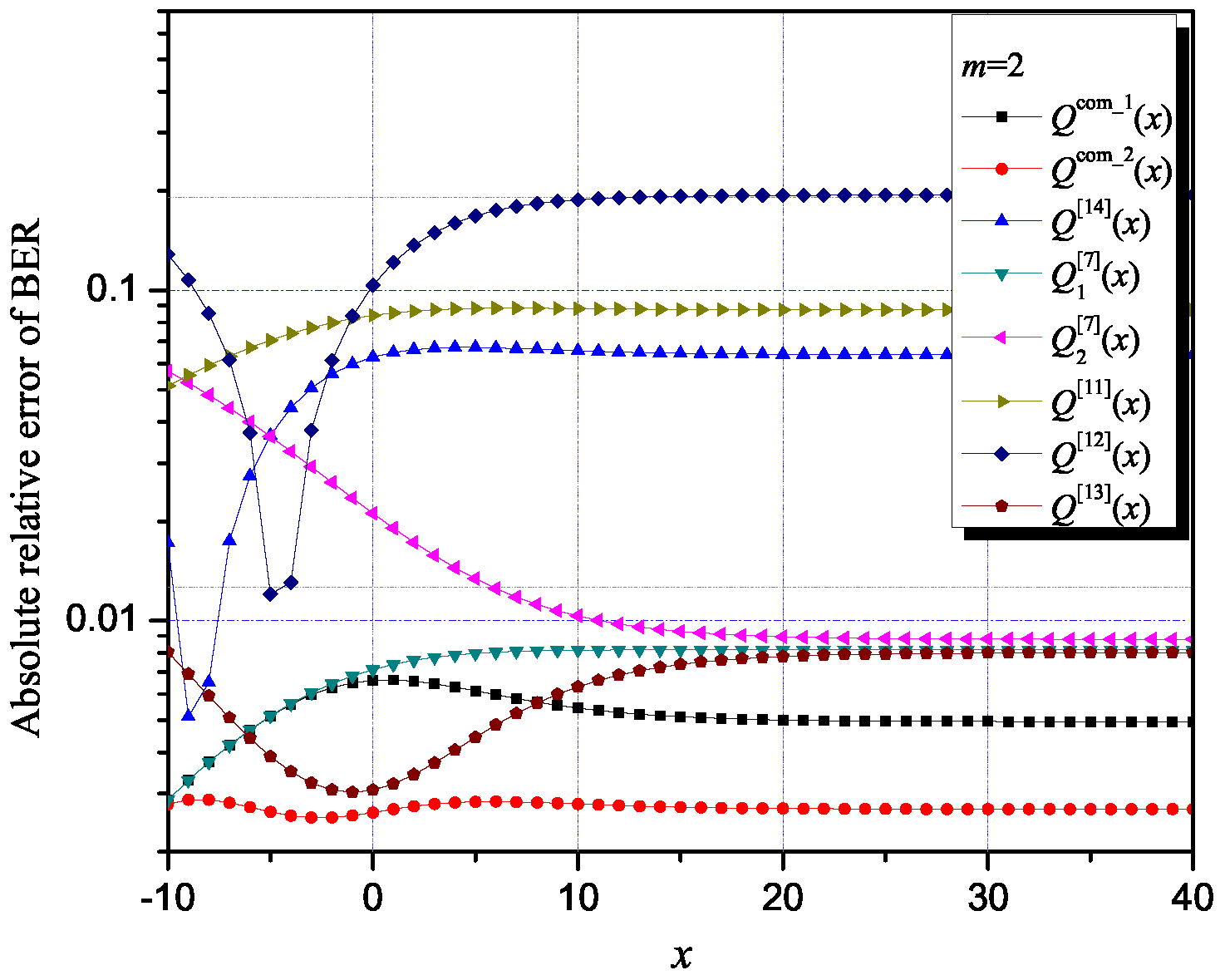
To point out an excellent match of the values of the ASEP for a BPSK modulation, calculated with the proposed composite approximations Q${}^{com\_2}$(x) and Q${}^{com\_1}$(x), and the exact ones, in Figure 4, we present the values for the absolute relative error of the BER for m = 2. By using Q${}^{com\_2}$(x) and Q${}^{com\_1}$(x), very tight approximations (lower values of the absolute error of BER) were obtained in a wide range of argument values compared to cases utilizing the Q-function approximations from the literature selected for comparison purposes and used for the ASEP values computation.

Our proposed Q-function approximations can also be applied for the ASEP evaluation for the assumed differentially encoded quadrature phase-shift keying (DE-QPSK) modulation format and Nakagami-m fading channels. The ASEP of DE-QPSK is given by [31]

$$P_b={\int }_0^{\infty }\overline{P_b}·f_{\gamma }\left(\gamma \right)d\gamma ,$$

(15)

where $f_{\gamma }\left(\gamma \right)$ is the Nakagami-m PDF of the signal-to-noise ratio (SNR) per symbol, distributed as specified in [32]:

$$f_{\gamma }\left(\gamma \right)=\frac{m^m}{\Gamma \left(m\right){\overline{\gamma }}^m}{\gamma }^{m-1}exp\left\{-m\frac{\gamma }{\overline{\gamma }}\right\},$$

(16)

and

$$\overline{P_b}=4Q\left(\sqrt{\gamma }\right)-8Q^2\left(\sqrt{\gamma }\right)+8Q^3\left(\sqrt{\gamma }\right)-4Q^4\left(\sqrt{\gamma }\right),$$

(17)

where $\overline{\gamma }$ represents the average SNR per symbol. As is well-known from the telecommunication theory, the relation between the received carrier amplitude under fading influence x, its mean squared value $\mathrm{\Omega }$, and the instantaneous signal-to-noise power ratio (SNR) per symbol, $\gamma$, is given with $\gamma =x^2\overline{\gamma }/\mathrm{\Omega }$. Similarly, the PDF of $\gamma$ could be obtained by introducing a change of variables in the expression for the fading amplitude PDF, p${}_x$(x), yielding [19]:

$$p_{\gamma }\left(\gamma \right)=p\left(\sqrt{\gamma \frac{\mathrm{\Omega }}{\overline{\gamma }}}\right)\left|J\right|,$$

(18)

and

$$\left|J\right|=\frac{dx}{d\gamma }=\frac{1}{2\sqrt{\gamma \frac{\overline{\gamma }}{\mathrm{\Omega }}}}.$$

(19)

A comparison of the exact and approximated values of the ASEP for the DE-QPSK modulation are presented in

Table 6. Values of the exact and approximated ASEP of the DE-QPSK for parameter m = 2.5.

E${}_{\mathit{b}}$N${}_0$ (dB)	Exact (m = 2.5)	Q${}^{com\_2}$(x)	Q${}^{com\_1}$(x)	Q${}^{\left[14\right]}$ (x)	Q${}^{\left[11\right]}$(x)	Q${}^{\left[12\right]}$ (x)	Q${}^{\left[13\right]}$ (x)	Q${}_1{}^{\left[7\right]}$(x)	Q${}_2{}^{\left[7\right]}$ (x)
−10	$7.1833\times {10}^{-1}$	$7.1872\times {10}^{-1}$	$7.188\times {10}^{-1}$	$7.0980\times {10}^{-1}$	$7.2608\times {10}^{-1}$	$6.7508\times {10}^{-1}$	$7.2013\times {10}^{-1}$	$7.1873\times {10}^{-1}$	$7.2865\times {10}^{-1}$
0	$4.8137\times {10}^{-1}$	$4.8220\times {10}^{-1}$	$4.8344\times {10}^{-1}$	$4.9996\times {10}^{-1}$	$5.0492\times {10}^{-1}$	$5.0609\times {10}^{-1}$	$4.8222\times {10}^{-1}$	$4.8340\times {10}^{-1}$	$4.8760\times {10}^{-1}$
10	$0.4325\times {10}^{-1}$	$0.4338\times {10}^{-1}$	$0.4344\times {10}^{-1}$	$0.4570\times {10}^{-1}$	$0.4655\times {10}^{-1}$	$0.5122\times {10}^{-1}$	$0.4352\times {10}^{-1}$	$0.4357\times {10}^{-1}$	$0.4350\times {10}^{-1}$
20	$3.0977\times {10}^{-4}$	$3.1053\times {10}^{-4}$	$3.1074\times {10}^{-4}$	$3.2642\times {10}^{-4}$	$3.3358\times {10}^{-4}$	$3.6930\times {10}^{-4}$	$3.1288\times {10}^{-4}$	$3.1196\times {10}^{-4}$	$3.1095\times {10}^{-4}$
30	$1.0814\times {10}^{-6}$	$1.0838\times {10}^{-6}$	$1.0845\times {10}^{-6}$	$1.1389\times {10}^{-6}$	$1.1642\times {10}^{-6}$	$1.2888\times {10}^{-6}$	$1.0928\times {10}^{-6}$	$1.0889\times {10}^{-6}$	$1.0851\times {10}^{-6}$
40	$3.4546\times {10}^{-9}$	$3.4621\times {10}^{-9}$	$3.4642\times {10}^{-9}$	$3.6378\times {10}^{-9}$	$3.7190\times {10}^{-9}$	$4.1169\times {10}^{-9}$	$3.4911\times {10}^{-9}$	$3.4783\times {10}^{-9}$	$3.4664\times {10}^{-9}$

,

Table 7. Values of the exact and approximated ASEP of the DE-QPSK for parameter m = 3.5.

E${}_{\mathit{b}}$N${}_0$ (dB)	Exact (m = 3.5)	Q${}^{com\_2}$(x)	Q${}^{com\_1}$(x)	Q${}^{\left[14\right]}$ (x)	Q${}^{\left[11\right]}$(x)	Q${}^{\left[12\right]}$ (x)	Q${}^{\left[13\right]}$ (x)	Q${}_1{}^{\left[7\right]}$(x)	Q${}_2{}^{\left[7\right]}$ (x)
−10	$7.1831\times {10}^{-1}$	$7.1870\times {10}^{-1}$	$7.1880\times {10}^{-1}$	$7.0995\times {10}^{-1}$	$7.2617\times {10}^{-1}$	$6.7514\times {10}^{-1}$	$7.2012\times {10}^{-1}$	$7.1871\times {10}^{-1}$	$7.2893\times {10}^{-1}$
0	$4.7634\times {10}^{-1}$	$4.7716\times {10}^{-1}$	$4.7854\times {10}^{-1}$	$4.9639\times {10}^{-1}$	$5.0089\times {10}^{-1}$	$5.0448\times {10}^{-1}$	$4.7717\times {10}^{-1}$	$4.7848\times {10}^{-1}$	$4.8237\times {10}^{-1}$
10	$0.2889\times {10}^{-1}$	$0.2898\times {10}^{-1}$	$2.9003\times {10}^{-2}$	$0.3053\times {10}^{-1}$	$0.3119\times {10}^{-1}$	$0.3479\times {10}^{-1}$	$0.2913\times {10}^{-1}$	$0.2911\times {10}^{-1}$	$0.2901\times {10}^{-1}$
20	$4.0809\times {10}^{-5}$	$4.0824\times {10}^{-5}$	$4.0833\times {10}^{-5}$	$4.2775\times {10}^{-5}$	$4.3866\times {10}^{-5}$	$4.8609\times {10}^{-5}$	$4.1412\times {10}^{-5}$	$4.1042\times {10}^{-5}$	$4.0838\times {10}^{-4}$
30	$1.5659\times {10}^{-8}$	$1.5645\times {10}^{-8}$	$1.5648\times {10}^{-8}$	$1.6377\times {10}^{-8}$	$1.6800\times {10}^{-8}$	$1.8571\times {10}^{-58}$	$1.5894\times {10}^{-8}$	$1.5728\times {10}^{-8}$	$1.5649\times {10}^{-6}$
40	$5.052\times {10}^{-12}$	$5.049\times {10}^{-12}$	$5.047\times {10}^{-12}$	$5.282\times {10}^{-12}$	$5.418\times {10}^{-12}$	$5.988\times {10}^{-12}$	$5.127\times {10}^{-12}$	$5.073\times {10}^{-12}$	$5.048\times {10}^{-9}$

and

Table 8. Values of the exact and approximated ASEP of the DE-QPSK for parameter m = 4.5.

E${}_{\mathit{b}}$N${}_0$ (dB)	Exact (m = 2.5)	Q${}^{com\_2}$(x)	Q${}^{com\_1}$(x)	Q${}^{\left[14\right]}$ (x)	Q${}^{\left[11\right]}$(x)	Q${}^{\left[12\right]}$ (x)	Q${}^{\left[13\right]}$ (x)	Q${}_1{}^{\left[7\right]}$(x)	Q${}_2{}^{\left[7\right]}$ (x)
−10	$7.1829\times {10}^{-1}$	$7.1869\times {10}^{-1}$	$7.188\times {10}^{-1}$	$7.1004\times {10}^{-1}$	$7.2622\times {10}^{-1}$	$6.7517\times {10}^{-1}$	$7.2011\times {10}^{-1}$	$7.1870\times {10}^{-1}$	$7.2908\times {10}^{-1}$
0	$4.7344\times {10}^{-1}$	$4.7420\times {10}^{-1}$	$4.7572\times {10}^{-1}$	$4.9435\times {10}^{-1}$	$4.9859\times {10}^{-1}$	$5.0365\times {10}^{-1}$	$4.7424\times {10}^{-1}$	$4.7564\times {10}^{-1}$	$4.7934\times {10}^{-1}$
10	$0.2154\times {10}^{-1}$	$0.2160\times {10}^{-1}$	$2.1611\times {10}^{-2}$	$0.2273\times {10}^{-1}$	$0.2327\times {10}^{-1}$	$0.2610\times {10}^{-1}$	$0.2176\times {10}^{-1}$	$0.2171\times {10}^{-1}$	$0.2161\times {10}^{-1}$
20	$6.9898\times {10}^{-6}$	$6.9988\times {10}^{-6}$	$7.1100\times {10}^{-6}$	$7.2615\times {10}^{-6}$	$7.4592\times {10}^{-6}$	$8.1755\times {10}^{-6}$	$7.1104\times {10}^{-6}$	$6.9990\times {10}^{-6}$	$6.9595\times {10}^{-6}$
30	$3.043\times {10}^{-10}$	$3.017\times {10}^{-10}$	$3.015\times {10}^{-10}$	$3.142\times {10}^{-10}$	$3.227\times {10}^{-10}$	$3.519\times {10}^{-10}$	$3.087\times {10}^{-10}$	$3.015\times {10}^{-10}$	$3.015\times {10}^{-10}$
40	$9.949\times {10}^{-15}$	$9.854\times {10}^{-15}$	$9.851\times {10}^{-15}$	$1.026\times {10}^{-14}$	$1.054\times {10}^{-14}$	$1.149\times {10}^{-14}$	$1.009\times {10}^{-14}$	$9.851\times {10}^{-15}$	$9.850\times {10}^{-15}$

. The exact values of the ASEP were calculated by means of numerical integration using Equation (1). For determining the approximated values, Equations (10) and (11) were applied as well as the corresponding ones from the literature, carefully chosen for comparison purposes.

From Table 6, Table 7 and Table 8 and Figure 5, it can be concluded that the approximate values of the ASEP for DE-QPSK over Nakagami-m fading channels could be efficiently and precisely evaluated for different values of the parameter m by utilizing the proposed approximations. By using the approximations of the Q-function given by Equations (10) and (11), the ABER measures were bounded more closely than by using the closed-form Q-function approximations selected from the literature, in the whole range of fading conditions.

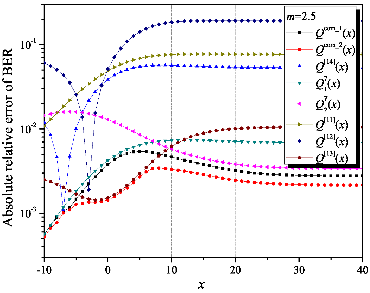
Figure 5 presents the values of the absolute relative error of the ASEP DE-QPSK approximations for a Nakagami-m channel and m = 2.5, to point out the smallest possible deviation of the approximated ASEP DE-QPSK values from the exact ones in case of applying the proposed Q-function approximations. In other words, the presented results provide an additional justification for the benefits of using the proposed composite improved interval approximation of the Q-function (our second upper bound composite interval approximation of the Q-function) in designing wireless communication systems for an accurate estimation of the expected QoS (quality of service).

6. Application in Designing a Quantizer with Equiprobable Cells for Gaussian Sources

Let x be a Gaussian random variable with probability density function:

$$p\left(x\right)=\frac{1}{\sqrt{2\pi }}exp\left\{-\frac{x^2}{2}\right\},-\infty <x<+\infty .$$

(20)

To represent this variable with a finite number of bits R, the range of possible amplitude values ($-\infty$, +∞) should be partitioned into $N=2^R$ disjoint cells, whereby one representation value should be assigned to each cell. Due to the symmetry of the Gaussian probability density function, the symmetry should also exist in the quantization, allowing us to observe only a partition of the amplitude range for positive values. Therefore, let $t_i$, $i=0,1,...,N$ be the thresholds that partition the positive part of the amplitude range and let $y_i$, $i=1,2,\dots ,N$ be the representation levels, whereby it holds that $t_0<y_1<t_1<y_2<\dots <t_{N/2-1}<y_{N/2-1}<t_{N/2}$ and $t_0$=0, $t_{N/2}=+\infty$. Then, quantization $F_Q$ is the following function:

$$F_Q\left(x\right)=y_{i}sgn\left(x\right)\mathrm{if}{t}_{i-1}\le \left|x\right|<t_i,$$

(21)

where $sgn\left(\right)$ is the sign function. In other words, the quantization transforms a variable x into F${}_Q$(x), producing the error x−F${}_Q$(x). Then, the performance of the quantization can be measured by estimating the mean squared error or distortion D:

$$D=\frac{1}{M}\sum _{i=1}^M{\left(x_i-y_i\right)}^2$$

(22)

and the signal-to-quantization-noise ratio SQNR:

$$\mathrm{SQNR}=\frac{{\sum }_{i=1}^M{x}_i^2}{{\sum }_{i=1}^M{\left(x_i-y_i\right)}^2},$$

(23)

where M is a big enough number of variables.

Based on the above, it is clear that a symmetric N-level quantization is defined with thresholds $t_i$, $i=0,1,\dots ,N/2$ and representation levels $y_i$, $i=1,2,\dots ,N/2$, which means that the quantization design involves the determination of these levels subject to a certain criterion. In the literature the commonly used criterion is the minimum distortion or a constant signal-to-quantization-noise ratio, while in this paper, as in [24], we designed the quantization subject to the criterion that the probability of a variable with a Gaussian probability density function belonging to a cell is the same for all cells. Actually, we focused on providing a quantization with equiprobable cells. In doing so, we encountered the Q-function. Namely, the probability that a variable having a Gaussian probability density function belonged to a certain cell was:

$$P_i={\int }_{t_i-1}^{t_i}p\left(x\right)dx=Q\left(t_{i-1}\right)-Q\left(t_i\right)=\frac{1}{N},i=1,2,\dots ,N/\phantom{N2}2$$

(24)

thus forming a systems of N/2-1 integral equations that should be solved per $t_i$, $i=1,\dots ,\mathit{N}/2-2$, since $t_0$ = 0 and $t_{N/2}$ = +∞ implies Q(t${}_0$) = 1/2 and Q(t${}_N$${}_{/2}$) = 0:

$$Q\left(t_i\right)=\frac{1}{\sqrt{2\pi }}{\int }_{t_i}^{+\infty }exp\left\{-\frac{x^2}{2}\right\}dx=\frac{N-2i}{2N},i=1,2,\dots ,N/\phantom{N2}2-1.$$

(25)

Using a closed-form approximation for the Q-function can reduce the complexity of the above system of equations, which is what we did in this paper by applying the composite upper-bound approximation given by (10):

$$Q^{\mathrm{com}\_1}\left(t_i\right)=\frac{N-2i}{2N},i=1,2,\dots ,N/\phantom{N2}2-1.$$

(26)

After that, we solved the resulting system of nonlinear equations using the bisection method.

Similarly, we determined the representation levels from the condition that $Q\left(y_i\right)$ were in the middle between $Q\left(t_{i-1}\right)$ and $Q\left(t_i\right)$, forming in that manner a system of N/2 integral equations, that could be solved as was previously described, that is, by solving the following system of equations:

$$Q^{com\_1}\left(y_i\right)=\frac{N-2i+1}{2N},i=1,2,\dots ,N/\phantom{N2}2.$$

(27)

The results we obtained for the design parameters using the Q-function approximation are presented in

Table 9. Scalar quantization designed to have equiprobable cells when quantizing a Gaussian variable with zero mean value and unit variance.

R (Bits/Sample)	${\mathit{x}}_{\mathit{i}}$, $\mathit{i}=0,1,\mathit{\dots },\mathit{N}/2$	${\mathit{y}}_{\mathit{i}}$, $\mathit{i}=1,\mathit{\dots },\mathit{N}/2$	D	SQNR (dB)
2	0		0.1458	8.36
	0.6787	0.3205
	+∞	1.1555
3	0		0.0578	12.38
	0.3207	0.1582
	0.6788	0.4924
	1.1551	0.8923
	+∞	1.5375
4	0		0.0235	16.30
	0.1581	0.0788
	0.3203	0.2383
	0.4923	0.4053
	0.6789	0.5830
	0.8923	0.7810
	1.1553	1.0148
	1.5371	1.3227
	+∞	1.8646

. In addition to the design parameters, Table 9 also tabulates the values for the distortion and signal-to-quantization-noise ratio estimated by running a simulation of the proposed quantization. In the Matlab software package, we generated and quantized according to Equation (21) M = 10${}^8$ Gaussian variables. By comparing the generated and quantized values, as Equations (22) and (23) specify, we estimated the quantization performance for bit rates of 2, 3 and 4 bits/sample.

The approximation of the Q-function has a wide range of applications. We listed two. It can be applied in all areas where data are modeled by a Gaussian PDF. Further, the theory of quantization, besides big data theory, can be used in neural networks, MIMO systems, signal transmission, 5G networks, as well as in Internet-of-things source coding. The Gaussian PDF is the most common data model encountered and also has applications in signal processing. A further application of the proposed approximation can be considered in areas described in [33,34,35,36,37,38]. Some of these applications will be the focus of our future research.

7. Conclusions

In this paper, two novel interval upper-bound approximations of the Q-function were proposed. The first one had a simpler analytical form and, therefore, could be applied in a simpler manner, whereas the second one was more accurate. In addition, by comparing both approximations with the Q-function approximations of similar analytical forms from the literature, we ascertained noticeable improvements in terms of the accuracy achieved by the proposed interval upper-bound approximations of the Q-function in the whole domain of the function argument.

In addition, comparisons of the estimated ASEP values for Nakagami-m fading channels for several values of parameter m were given in the paper for two modulation types, BPSK and DE-QPSK, to demonstrate the usefulness of the proposed Q-function approximations. Furthermore, we showed that the closed-form approximation of the Q-function could be used in the quantization design for variables from Gaussian sources, whereby using the closed-form Q-function approximation avoided solving the integral equations. Another advantage of the new composite approximation formulas was a very small increase in computational complexity. That made them suitable for various applications including the analysis of the performance of various communication channels.

In brief, for the observed applications, we showed the superiority of our proposal over the Q-function approximations previously used in the literature, considered in the paper for comparison purposes. Due to the relatively small absolute relative errors that the novel Q-function approximations provide, we can anticipate that they can find applications in a variety of problems encountered not only in communication theory, but also in a number of analyses involving the estimation of the Q-function.

References

1. Panić, S.; Stefanović, M.; Anastasov, J.; Spalević, P. Fading and Interference Mitigation in Wireless Communications, 1st ed.; CRC Press: Boca Raton, FL, USA, 2013. [Google Scholar]
2. Aggarwal, S. A survey-cum-tutorial on approximations to Gaussian Q-function for symbol error probability analysis over Nakagami- m fading channels. IEEE Commun. Surv. Tutor. 2019, 21, 2195–2223. [Google Scholar] [CrossRef]
3. Sadhwani, D.; Yadav, R.N.; Aggarwal, S. Tighter bounds on the Gaussian Q function and its application in Nakagami-m fading channel. IEEE Wirel. Commun. Lett. 2017, 6, 574–577. [Google Scholar] [CrossRef]
4. Marković, A.V.; Perić, Z.H.; Panić, S.R.; Spalević, P.C.; Prlincević B., P. An improved method for ASEP evaluation over fading channels based on Q-function approximation. IETE J. Res. 2018, 64, 777–784. [Google Scholar] [CrossRef]
5. Aggarwal, S. Application of Gaussian Q-function approximations in fluctuating Beckmann fading model. Natl. Acad. Sci. Lett. 2021, 44, 125–131. [Google Scholar] [CrossRef]
6. Rubio, L.; Reig, J.; Cardona, N. Evaluation of Nakagami fading behavior based on measurements in urban scenarios. Int. J. Electron. Commun. 2007, 61, 135–138. [Google Scholar] [CrossRef]
7. Gasull, A.; Utzet, F. Approximating Mills ratio. J. Math. Anal. Appl. 2014, 420, 1832–1853. [Google Scholar] [CrossRef] [Green Version]
8. Yang, Z.H.; Chu, Y.M. On approximating Mills ratio. J. Inequalities Appl. 2015, 2015, 273. [Google Scholar] [CrossRef] [Green Version]
9. Shi, Q.; Karasawa, Y. An accurate and efficient approximation to the Gaussian Q-function and its applications in performance analysis in Nakagami-m fading. IEEE Commun. Lett. 2011, 15, 479–481. [Google Scholar]
10. Tellambura, C.; Annamalai, A. Efficient computation of erfc(x) for large arguments. IEEE Trans. Commun. 2000, 48, 529–532. [Google Scholar] [CrossRef] [Green Version]
11. Jang, W.M. A simple upper bound of the Gaussian Q-function with closed-form error bound. IEEE Commun. Lett. 2011, 15, 157–159. [Google Scholar] [CrossRef]
12. Chiani, M.; Dardari, D.; Simon, M.K. New exponential bounds and approximations for the computation of error probability in fading channels. IEEE Trans. Wirel. Commun. 2003, 2, 840–845. [Google Scholar] [CrossRef] [Green Version]
13. Abreu, G. Very simple tight bounds on the Q-function. IEEE Trans. Commun. 2012, 60, 2415–2420. [Google Scholar] [CrossRef]
14. Borjesson, P.O.; Sundberg, C.E. Simple approximations of the error function Q(x) for communications applications. IEEE Trans. Commun. 1979, 27, 639–643. [Google Scholar] [CrossRef]
15. Karagiannidis, G.K.; Lioumpas, A.S. An improved approximation for the Gaussian Q-function. IEEE Commun. Lett. 2007, 11, 644–646. [Google Scholar] [CrossRef]
16. Nikolić, J.; Perić, Z.; Jovanović, A. Novel approximations for the Q-function with application in SQNR calculation. Digit. Signal Process. 2017, 65, 71–80. [Google Scholar] [CrossRef]
17. Perić, Z.; Nikolić, J.; Petković, M.D. Class of tight bounds on the Q-function with closed-form upper bound on relative error. Math. Methods Appl. Sci. 2019, 42, 1786–1794. [Google Scholar] [CrossRef]
18. Tegos, S.A.; Tyrovolas, D.; Diamantoulakis, P.D.; Liaskos, C.K.; Karagiannidis, G.K. On the Distribution of the Sum of Double-Nakagami-m Random Vectors and Application in Randomly Reconfigurable Surfaces. IEEE Trans. Veh. Technol. 2022, 71, 7297–7307. [Google Scholar] [CrossRef]
19. Panajotovic, A.S.; Sekulovic, N.M.; Stefanovic, M.C.; Draca, D.L. Average Level Crossing Rate of Dual Selection Diversity over Correlated Unbalanced Nakagami-m Fading Channels in the Presence of Cochannel Interference. IEEE Commun. Lett. 2012, 16, 691–693. [Google Scholar] [CrossRef]
20. Stefanovic, C.; Milovanovic, I.; Panic, S.; Stefanovic, M. LCR and AFD of the Products of Nakagami-m and Nakagami-m Squared Random Variables: Application to Wireless Communications Through Relays. Wirel. Pers. Commun. 2022, 123, 2665–2678. [Google Scholar] [CrossRef]
21. Peric, Z.H.; Markovic, A.V.; Kontrec, N.; Panic, S.R.; Spalević, P.C. Novel Composite Approximation for the Gaussian Q-Function. Elektronika ir Elektrotechnika 2020, 26, 33–38. [Google Scholar] [CrossRef]
22. Markovic, A.; Peric, Z.; Panic, S.; Spalevic, P.; Todorovic, Z. Improved Composite Q-Function Approximation and its Aplication in ASEP of Digital Modulations over Fading Channels. Elektronika ir Elektrotechnika 2017, 23, 83–88. [Google Scholar] [CrossRef] [Green Version]
23. Markovic, A.; Peric, Z.; Panic, S.; Spalevic, P. Average Bit Error Rate Calculation on Piecewise Spline Approximation. Rev. Roum. Sci. Techn. Électrotechn. Énerg 2019, 64, 255–258. [Google Scholar]
24. Baskin, C.; Liss, N.; Schwartz, E.; Zheltonozhskii, E.; Giryes, R.; Bronstein, A.M.; Mendelson, A. UNIQ: Uniform Noise Injection for Non-Uniform Quantization of Neural Networks. Acm Trans. Comput. Syst. 2019, 37, 1–15. [Google Scholar] [CrossRef]
25. Abramowitz, M.; Stegun, I.A. Handbook of Mathematical Functions: With Formulas, graphs, and Mathematical Tables; National Bureau of Standards: Washington, DC, USA, 1970. [Google Scholar]
26. Simon, M.K. Probability Distributions Involving Gaussian Random Variables: A Handbook for Engineers and Scientists; Springer: New York, NY, USA, 2006. [Google Scholar]
27. Nikolić, J.; Perić, Z.; Marković, A. Proposal of simple and accurate two-parametric approximation for the Q-function. Math. Probl. Eng. 2017, 2017, 8140487. [Google Scholar] [CrossRef] [Green Version]
28. Gradshteyn, I.S.; Ryzhik, I.M. Tables of Integrals, Series and Products, 5th ed.; Academic Press: San Diego, CA, USA, 1994. [Google Scholar]
29. Lakhzouri, A.; Lohan, E.; Saastamoinen, I.; Renfors, M. Measurement and characterization of satellite-to-indoor radio wave propagation channel. In Proceedings of the European Navigation Conference GNSS 2005, Munich, Germany, 19–22 July 2005; pp. 1–6. [Google Scholar]
30. Selim, B.; Alhussein, O.; Muhaidat, S.; Karagiannidis, G.; Liang, J. Modeling and analysis of wireless channels via the mixture of Gaussian distribution. IEEE Trans. Veh. Technol. 2016, 65, 8309–8321. [Google Scholar] [CrossRef] [Green Version]
31. Youssef, N.; El Bahri, W.; Patzold, M.; El Asmi, S. On the crossing statistics of phase processes and random FM noise in Nakagami-q mobile fading channels. IEEE Trans. Wirel. Commun. 2005, 4, 24–29. [Google Scholar] [CrossRef]
32. Simon, M.K. Single integral representations of certain integer powers of the Gaussian Q-function and their application. IEEE Commun. Lett. 2002, 6, 532–534. [Google Scholar] [CrossRef]
33. Li, H.; Ota, K.; Dong, M.; Guo, M. Learning Human Activities through Wi-Fi Channel State Information with Multiple Access Points. IEEE Commun. Mag. 2018, 56, 124–129. [Google Scholar] [CrossRef] [Green Version]
34. Wang, J.; Yang, Y.; Wang, T.; Sherratt, R.; Zhang, J. Big Data Service Architecture: A Survey. J. Internet Technol. 2020, 21, 393–405. [Google Scholar]
35. Ke, H.; Li, P.; Guo, S.; Guo, M. On Traffic-Aware Partition and Aggregation in MapReduce fo Big Data Applications. IEEE Trans. Parallel Distrib. Syst. 2016, 27, 818–828. [Google Scholar] [CrossRef]
36. Pu, B.; Li, K.; Li, S.; Zhu, N. Automatic Fetal Ultrasound Standard Plane Recognition Based on Deep Learning and IIoT. IEEE Trans. Ind. Inform. 2021, 17, 7771–7780. [Google Scholar] [CrossRef]
37. Zhang, J.; Zhong, S.; Wang, T.; Chao, H.C.; Wang, J. Blockchain-Based Systems and Applications: A Survey. J. Internet Technol. 2020, 21, 1–14. [Google Scholar]
38. Gao, J.; Lin, X. Mathematical interpolation and correction of three-dimensional modelling of high-speed railway. Intell. Autom. Soft Comput. 2020, 5, 1023–1034. [Google Scholar] [CrossRef]
Figure 1. Comparison of several Q-function approximations.
Mathematics 10 03590 g001
Figure 2. The comparison of the absolute relative errors of the first interval upper-bound approximation of the Q-function and selected ones from the literature [7,11,12,13,14].
Mathematics 10 03590 g002
Figure 3. The comparison of the absolute relative errors of the two novel interval upper-bound approximations of the Q-function with the one from [13].
Mathematics 10 03590 g003
Figure 4. Absolute relative error of determining ASEP for BPSK modulation: comparison of the applied proposed approximations and the selected ones from the literature.
Mathematics 10 03590 g004
Figure 5. Absolute relative error of determining ASEP for DE-QPSK modulation: comparison of the applied proposed approximations and the selected ones from the literature.
Mathematics 10 03590 g005