A Weighted Surrogate Model for Spatio-Temporal Dynamics with Multiple Time Spans: Applications for the Pollutant Concentration of the Bai River

Abstract

Simulations are often used to investigate the flow structures and system dynamics of complex natural phenomena and systems, which are significantly harder to obtain from experiments or theoretical analyses. Surrogate models are employed to mimic the results of simulations by reducing computational costs. In order to reduce the amount of computational time consumed, a novel framework for building efficient surrogate models is proposed in this work. The novelty lies in that the new framework runs simulations using the different simulation time spans for different inputs and builds a comprehensive surrogate model through the fusion of non-homogeneous spatio-temporal data by integrating the temporal and spatial correlations in parametric space. This differs from the existing works in the literature, which only consider the situation of spatio-temporal data with a consistent time span during simulations under different inputs. Some simulation studies and real data analysis concerning the pollution of the river in the Sichuan Province of China are used to demonstrate the superior performance of the proposed methods.

1. Introduction

In practice, partial differential equations (PDEs) are often employed to study complex natural phenomena and engineering systems in many fields, such as meteorology, turbulence, and aircraft design. Numerical methods, such as the finite element algorithm, are used to solve PDEs, referred to in the literature as simulators. High-fidelity simulations have been used for investigating system dynamics and flow structures. However, it is time-consuming to run the corresponding simulations. Modeling and estimating the spatio-temporal dynamics over a wide parametric space are important challenges that are yet to be overcome. Surrogate models are widely utilized to mimic the results of simulators with significantly reduced computational costs.

There have been many previous works building surrogate models for spatio-temporal dynamics in the literature. Xiao et al. [1] present a non-intrusive subdomain POD-TPWL (SD POD-TPWL) method through integral domain decomposition (DD), proper orthogonal decomposition (POD, which was first proposed by [2]), radial basis function (RBF) interpolation, and trajectory segmentation linearization (TPWL). Ioannidis et al. [3] proposed a graph-aware kernel kriged Kalman filtering (KKF) method accounting for the spatio-temporal variations. Nguyen et al. [4] and Shi et al. [5] modeled spatio-temporal dynamics using mixed-effects models. These methods only pay attention to spatio-temporal dynamics under fixed input parameters. For example, the authors of [1] investigated the spatio-temporal performance of the oil–water reservoir system at fixed values of initial pressure, initial saturation, etc., instead of studying the influence of input parameters on the spatio-temporal dynamics.

Several works have proposed modeling the relationship between the spatio-temporal dynamics and the input parameters. Guo and Hesthaven [6] proposed a data-driven reduced basis (RB) method for parameterized spatio-temporal modeling problems, which reduced the dimensions of training data by POD and then built the regression-based error surrogate model. Yeh et al. [7] used POD to decompose the spatio-temporal system of the flow field in the vortex ejector and then trained the kriging model for the reduced data, which can predict the system dynamics under any input parameter. Chang et al. [8,9] proposed new surrogate models named kernel-smoothed proper orthogonal decomposition (KSPOD) and common kernel-smoothed proper orthogonal decomposition (CKSPOD) to emulate spatio-temporally evolving flows.

In order to build a more economical surrogate model, most of the above works used the POD, a widely used reduced order modeling (ROM) method, to represent the spatio-temporal data at a controlled loss of accuracy. From a data-driven point of view, Yeh et al. [7] sampled a set of input parameters $\Theta \triangleq \{{\theta }_1,{\theta }_2,\cdots ,{\theta }_c\}$ and ran simulations to generate the spatio-temporal data of the flow field in the vortex ejector $y=f(x,t;\theta )$ for each $\theta \in \Theta$. Then $f(x,t;\theta )$ is approximated into K common POD modes ${\varphi }_k\left(x\right)$ with time-varying coefficients ${\beta }_k(t;\theta )$, that is

$$f(x,t;\theta )\approx \sum _{k=1}^K{\beta }_k(t;\theta )·{\varphi }_k\left(x\right),$$

(1)

with the reasonable expectation that the approximation becomes exact as $K=N$ [10], where ${\varphi }_k\left(x\right)$ is a spatial basis function, and ${\beta }_k(t;\theta )$, $k=1,2,\cdots ,K$ is the k-th time-varying coefficient under input parameter $\theta$ and time t, which describes the relationship between ${\varphi }_k\left(x\right)$ and $f(x,t;\theta )$ given $\theta$ and t. Given k and time step $t_m$, time-varying coefficients ${\beta }_k(t_m;\theta )$ can be seen as functions of the input variable $\theta$. Hence, the kriging model is established for every ${\beta }_k(t_m;\theta )$, $m=1,2,\cdots ,M$ and $k=1,2,\cdots ,K$. For any new parameter ${\theta }^{*}$ in the parameter space $\Omega$, the kriging model can give the prediction ${\hat{\beta }}_k(t_m;{\theta }^{*})$. Then, the prediction of the system dynamics under the new parameter is given by

$$\hat{f}(x,t;\theta )=\sum _{k=1}^K{\widehat{\beta }}_k(t;\theta )·{\varphi }_k\left(x\right).$$

(2)

Most of the existing works in the literature assume that the temporal resolution is fine [7] and build a surrogate model based on the same time span $\mathcal{T}$. Attention has not been paid to the time correlations; however, for some practical problems, there are correlations between different time steps, such as the incompressible fluid flow, see [6].

Let $[0,t_M]$ be the time span of interest to engineers. In practice, due to the limitations of computational time and resources, only a few parameters of the spatio-temporal data are simulated to the last time step $t_M$, and the others are only simulated to the $M_i$-th time steps $t_{M_i}$, $i=1,2,\cdots ,s$, $t_{M_1}<t_{M_2}<\cdots <t_{M_s}=t_M$. Hence, the spatio-temporal data with different time spans need to be fused to build a comprehensive surrogate model. In this way, computational resources and time can be saved to simulate the spatio-temporal data under more parameters. Let ${\mathcal{T}}_i\triangleq \{t_1,t_2,\cdots ,t_{M_i}\}$, $i=,1,2,\cdots ,s$, and $\mathcal{T}={\mathcal{T}}_s$. Assume c is the number of parameters required to run the simulations for the traditional methods. Let $s=2$. Let $c_1$ be the number of parameters under which the spatio-temporal data are simulated over ${\mathcal{T}}_1$, and $c_2$ be the number of parameters under which the spatio-temporal data are simulated over $\mathcal{T}$. $c_1$ and $c_2$ can be chosen appropriately such that $c_1\times t_{M_1}+c_2\times t_M\approx c\times t_M$ and $c_1+c_2>c>c_2$. Thus, under the same computing resources, more input parameters, and their corresponding spatio-temporal data will be considered, which leads to a more accurate surrogate model. Take the case study of pollutant concentration in Section 4 as an example, for each input, the simulation will take approximately 22 h on a computer with 72 Intel(R) Xeon(R) Gold 6254 CPU @ 3.10 GHz and 16 G memory. If the number of inputs is $c=20$, it will take 440 h with the full time span for all of the inputs. If the number of inputs with full time span simulation is $c_1=10$ and the number of inputs with half time span simulation is $c_2=20$, it will also take approximately 440 h. However, we collect the data for approximately 30 different inputs, which could benefit the accuracy of the surrogate model.

Consider the pollution supervision of rivers as an example. A simulator is generally established for the hydrological situation of the entire river basin, the relevant indicators of the source of pollutants are used as input parameters, and certain spatio-temporal data are generated. In daily supervision, the spatio-temporal field under certain parameters in a certain period of time ${\mathcal{T}}_1$ is simulated through the simulator. However, when there is an emergency, a quick response of the flow structures over ${\mathcal{T}}_2$, which exceeds ${\mathcal{T}}_1$, is required. Therefore, it is necessary to quickly generate the spatio-temporal data over ${\mathcal{T}}_2\setminus {\mathcal{T}}_1$ at fewer parameters and establish a surrogate model to determine the source of pollutants and predict the river’s pollution distribution. For this case, a surrogate model is needed that uses different time spans for training data. In this work, we monitor pollution in the Bai River as an example to demonstrate the effectiveness of the proposed methods.

The objective of this paper is to propose a framework to build a surrogate model for fusing spatio-temporal data with multiple time spans. In order to reduce the amount of computational time consumed, the new framework is used to run simulations using different simulation time spans for different inputs, and to build a comprehensive surrogate model through the fusion of non-homogeneous spatio-temporal data by integrating temporal and spatial correlations.

The remainder of this paper is organized as follows. A new predictive surrogate model to fuse spatio-temporal data over different time spans is presented in Section 2. In Section 3, some simulations are carried out to illustrate the performance of the proposed methods when the training data have different time spans. In Section 4, real data analysis for the pollution of rivers in the Sichuan Province of China is given. Conclusions are drawn in Section 5.

2. Methodology

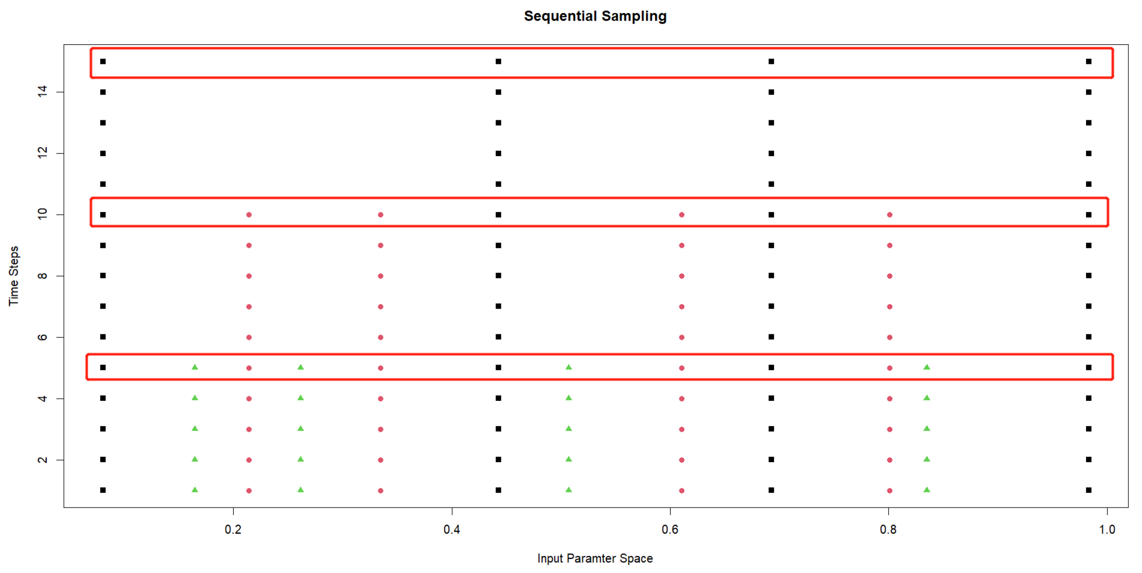
2.1. The Reverse Sequential Sampling Scheme

Usually, the spatio-temporal data are divided into N discrete spatial nodes $\mathcal{X}=\{x_1,x_2,\cdots ,x_N\}$ and M time steps $\mathcal{T}=\{t_1,t_2,\cdots ,t_M\}$. Suppose that there are s different time spans ${\mathcal{T}}_1\subset {\mathcal{T}}_2\subset \cdots \subset {\mathcal{T}}_s=\mathcal{T}$, which will be used in the simulations. Let the end of time span ${\mathcal{T}}_i$ be $t_{M_i}$, $i=1,2,\cdots ,s$ and assume that the time interval $\Delta t$ is the same over the entire time span. For each time span ${\mathcal{T}}_i$, $c_i$ input parameters are sampled from parameter space $\Omega$, and the corresponding spatio-temporal data are generated through the simulator. For spatio-temporal data at ${\mathcal{T}}_s\setminus {\mathcal{T}}_{s-1}\triangleq \{t_{M_{s-1}+1},t_{M_{s-1}+2},\cdots ,t_{M_s}\}$, there are only $c_s$ parameters available. For ${\mathcal{T}}_{s-1}\setminus {\mathcal{T}}_{s-2}$≜$\{t_{M_{s-2}+1},t_{M_{s-2}+2},\cdots ,t_{M_{s-1}}\}$, the number of parameters augment $c_s+c_{s-1}$. Thus, there are ${\sum }_{i=1}^s{c}_i$ training parameters, which is at a maximum over the first time span ${\mathcal{T}}_1=\{t_1,t_2,\cdots ,t_{M_1}\}$.

In order to ensure the prediction accuracy of the surrogate model, at each time point $t_m$, the selected parameters should have a good space-filling ability. Since the fewest training input parameters correspond to the spatio-temporal data at the time step $t\in \{t_{M_{s-1}+1},t_{M_{s-1}+2},\cdots ,t_{M_s}\}$, the selection of parameters over this time span should be prioritized. A feasible method is to uniformly sample $c_s$ parameters from the parameter space $\Omega$, which is denoted as ${\Theta }_s$. Then, using sequential Latin hypercube designs (LHDs), such as the Quasi-LHD sequential sampling method [11,12] and maximum projection (MaxPro) LHD [13,14], $c_{s-1}$ parameters are sampled from $\Omega \setminus {\Theta }_s$, the relative complement of ${\Theta }_s$ in $\Omega$, to compose ${\Theta }_{s-1}$, so that the parameters in ${\Theta }_s\cup {\Theta }_{s-1}$ have the space-filling property in $\Omega$. Continue this method until the sampling of ${\Theta }_1$ is finished. It is obvious that ${\Theta }_i\cap {\Theta }_j=\varnothing$, $1\cdots \le i<j\le \cdots s$. Let the j-th element in ${\Theta }_i$ be denoted as ${\theta }_{ij},j=1,2,\cdots c_i$. Then, the parameters in ${\Theta }_i$, $i=1,2,\cdots ,s$, are used to simulate the spatio-temporal data for ${\mathcal{T}}_i=\{t_1,t_2,\cdots ,t_{M_i}\}$. This method can sequentially generate spatio-temporal data with s different time spans for different input parameters, and the parameters have a good space-filling property in $\Omega$ and are uniform in each ${\Theta }_i$. In this paper, we refer to this sampling procedure as the reverse sequential sampling scheme, in which the “reverse” means that the order in which the parameters are sampled is the reverse of the order in which the simulator is run. The data simulation approach in this paper adopts the reverse sequential sampling scheme.

As an example to illustrate this method, 1-dimensional parameter space and time space are considered. The data with three time spans ${\mathcal{T}}_1=\{1,2,\cdots ,5\}$, ${\mathcal{T}}_2=\{1,2,\cdots ,10\}$, ${\mathcal{T}}_3=\{1,2,\cdots ,15\}$ and three parameter sets ${\Theta }_1$, ${\Theta }_2$, ${\Theta }_3\in [0,1]$ are generated. ${\Theta }_1=[0.16,0.25,0.50,0.84]$ was first sampled from $[0,1]$, such that the elements in ${\Theta }_1$ are uniform in $[0,1]$. Next ${\Theta }_2=[0.21,0.34,0.61,0.80]$ was sampled from $[0,1]\setminus {\Theta }_1$ to make sure that ${\Theta }_1\cup {\Theta }_2$ are uniform in $[0,1]$. Then, ${\Theta }_3=[0.04,0.44,0.69,0.98]$ was sampled to ensure the uniformity of ${\bigcup }_{i=2}^3{\Theta }_i$.

The parameters in ${\Theta }_1$,${\Theta }_2$, and ${\Theta }_3$ are represented as black, red, and green points in Figure 1, respectively. Each row in the figure represents the parameters at the corresponding time step. By using the reverse sequential sampling scheme, the training samples have good space filling in $[0,1]$, even though the number of training parameters decreased when $t\in {\Theta }_3\setminus {\Theta }_2=\{11,12,13,14,15\}$.

The collected dataset from all the ${\sum }_{i=1}^s{c}_i$ simulations is then used to train a surrogate model. Because there are many time steps and space nodes, building a surrogate model to respond at all temporal and spatial points is expensive. POD is a common method for reducing the dimensions of spatio-temporal data. For spatio-temporal data $f(x_n,t_m)$, $x_n$ represents a spatial node, and $t_m$ represents a time step. $\overline{f\left(x_n\right)}$ represents the average over the time steps of node $x_n$. Let $y(x_n,t_m)$ represent the spatio-temporal data minus the mean, i.e.,

$$y(x_n,t_m)=f(x_n,t_m)-\overline{f\left(x_n\right)},$$

(3)

and the spatio-temporal data can be denoted as

$$X\triangleq {\left[\begin{array}{ccc}y(x_1,t_1;\theta )& \cdots & y(x_1,t_M;\theta )\\ \cdots & \cdots & \cdots \\ y(x_N,t_1;\theta )& \cdots & y(x_N,t_M;\theta )\end{array}\right]}_{N\times M}.$$

(4)

Then, POD is used to decompose the real-valued $N\times N$ matrix $X{X}^T$ by eigenvalue decomposition. Let $\Phi =[{\varphi }_1,{\varphi }_2,\dots ,{\varphi }_N]$, where ${\varphi }_j\in {\mathbb{R}}^N$ is the standard orthogonal feature vector, and ${\lambda }_1,{\lambda }_2,\dots ,{\lambda }_N$ is the corresponding eigenmatrix and eigenvalues, respectively. The number of modes K is chosen such that $\frac{{\sum }_{i=1}^K{\lambda }_i}{{\sum }_{i=1}^n{\lambda }_i}\ge 99\%$, where the proportion of eigenvalue $\frac{{\lambda }_j}{{\sum }_{i=1}^N{\lambda }_i}$ represents the energy contained in the corresponding eigenvector ${\varphi }_j$. When considering that the spatio-temporal data removed the mean, $f(x,t)$ can be decomposed as

$$f(x,t)\approx \sum _{k=1}^K{\beta }_k\left(t\right){\varphi }_k,$$

(5)

where ${\beta }_k\left(t_m\right)$ is the time-varying coefficient corresponding to the k-th mode at time step $t_m$, which can be calculated by

$${\beta }_k\left(t_m\right)=<f\left(t_m\right),{\varphi }_k>,$$

(6)

where $f\left(t_m\right)={[f(x_1,t_m),f(x_2,t_m),\cdots ,f(x_N,t_m)]}^T$. Consider the modes $\{{\varphi }_1,{\varphi }_2,\dots ,{\varphi }_K\}$ as a common basis function, and the spatio-temporal data

$${\left[\begin{array}{ccc}f(x_1,t_1;{\theta }_{11})& \cdots & f(x_1,t_{M_1};{\theta }_{11})\\ \cdots & \cdots & \cdots \\ f(x_N,t_1;{\theta }_{11})& \cdots & f(x_N,t_{M_1};{\theta }_{11})\end{array}\right]}_{N\times M_1},\cdots ,{\left[\begin{array}{ccc}f(x_1,t_1;{\theta }_{s{c}_s})& \cdots & f(x_1,t_{M_1};{\theta }_{s{c}_s})\\ \cdots & \cdots & \cdots \\ f(x_N,t_1;{\theta }_{s{c}_s})& \cdots & f(x_N,t_{M_1};{\theta }_{s{c}_s})\end{array}\right]}_{N\times M_s}$$

(7)

can be represented by

$${\left[\begin{array}{ccc}{\beta }_1(t_1;{\theta }_{11})& \cdots & {\beta }_1(t_{M_1};{\theta }_{11})\\ \cdots & \cdots & \cdots \\ {\beta }_K(t_1;{\theta }_{11})& \cdots & {\beta }_K(t_{M_1};{\theta }_{11})\end{array}\right]}_{K\times M_1},\cdots ,{\left[\begin{array}{ccc}{\beta }_1(t_1;{\theta }_{s{c}_s})& \cdots & {\beta }_1(t_{M_1};{\theta }_{s{c}_s})\\ \cdots & \cdots & \cdots \\ {\beta }_K(t_1;{\theta }_{s{c}_s})& \cdots & {\beta }_K(t_{M_1};{\theta }_{s{c}_s})\end{array}\right]}_{K\times M_s}.$$

(8)

Note that, through the POD, the $N\times M$ dimensional matrix is reduced to the $K\times M$ dimensional matrix, which means that the spatio-temporal data with N space points and M time points are reduced from $N\times M$ to $K\times M$, where $N\gg K$.

2.2. The Proposed Model

After the decomposition of POD, the surrogate model can be built for each ${\beta }_k$ in (8). Since the establishment of the surrogate model is the same for every k, hereafter we omit k and let $\beta (t_m;\theta )$ denote ${\beta }_k(t_m;\theta )$. Section 2.2.1 will introduce the steps for building the surrogate model for $\beta (t_m;\theta ),j=1,2,\cdots ,t_{M_s}$. A weighted model is proposed in Section 2.2.2 to improve the stability of the model, and in Section 2.2.3, an algorithm to predict the system dynamics under new parameters is presented.

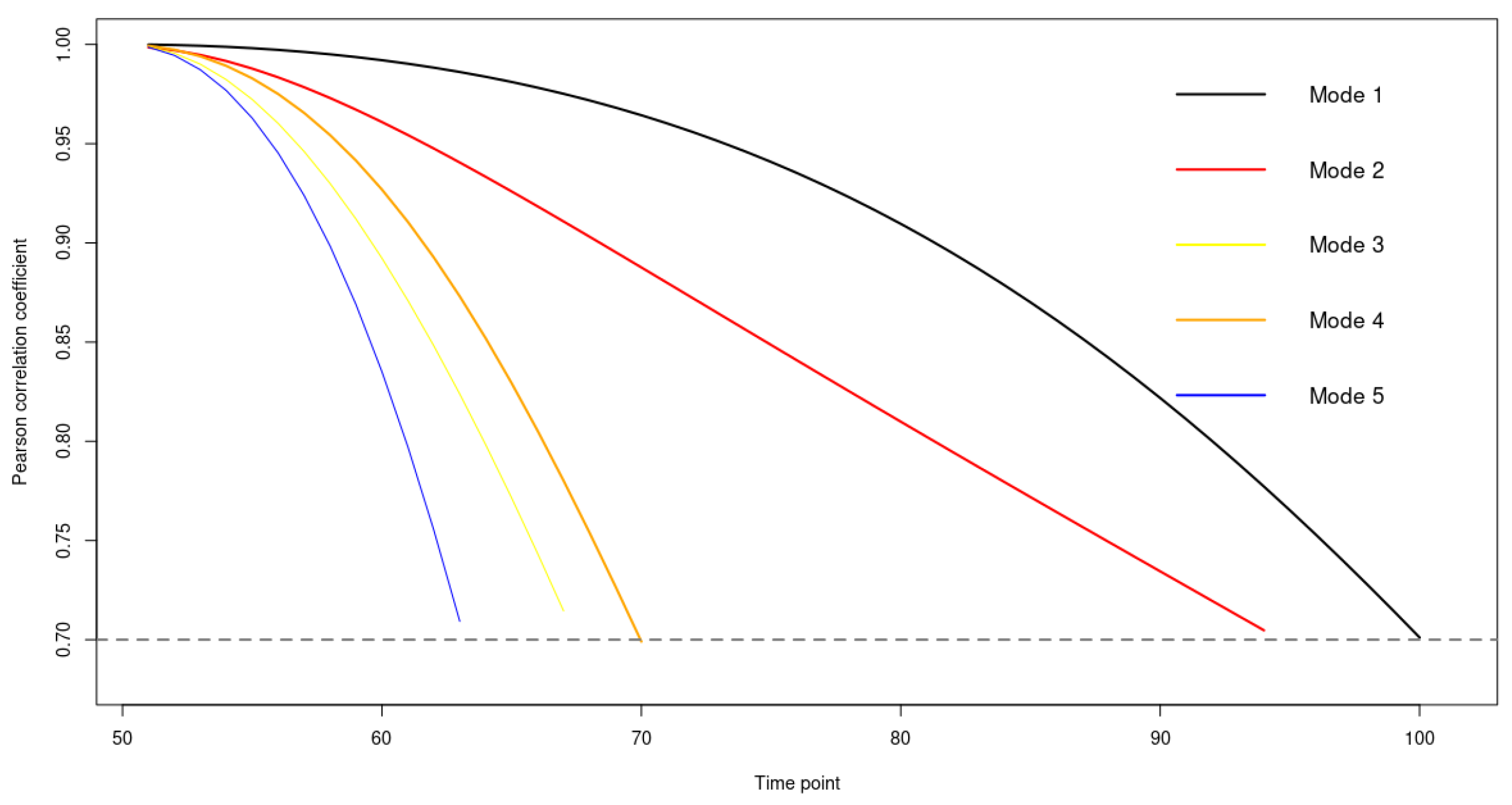
2.2.1. The Surrogate Model for Time-Varying Coefficients

To simplify the elaboration, we first introduce the proposed method with only two time spans ${\mathcal{T}}_1=\{t_1,t_2,\cdots ,t_{M_1}\}$ and ${\mathcal{T}}_2=\{t_1,t_2,\cdots ,t_{M_1},\cdots ,t_{M_2}\}$, where $t_{M_2}=t_M$. First, the $c_2$ and $c_1$ parameters are sequentially sampled from the parameter space $\Omega$ according to the algorithm proposed in the previous section and are denoted as ${\Theta }_2$ and ${\Theta }_1$, respectively. Each set of parameters ${\theta }_{2j}\in {\Theta }_2,j=1,2,\cdots c_2$ is plugged into the simulator to obtain the spatio-temporal field data $y=f(x,t),x=x_1,x_2,\cdots ,x_N$; $t=t_1,t_2,\cdots ,t_{M_1},t_{M_1+1},\cdots ,t_{M_2}$. For each set of parameters ${\theta }_{1j}\in {\Theta }_1,j=1,2,\cdots c_1$, corresponding simulations are made over $[0,t_{M_1}]$. Then, we have

$${\left[\begin{array}{ccc}\beta (t_1;{\theta }_{11})& \cdots & \beta (t_{M_1};{\theta }_{11})\\ \beta (t_1;{\theta }_{12})& \cdots & \beta (t_{M_1};{\theta }_{12})\\ \cdots & \cdots & \cdots \\ \beta (t_1;{\theta }_{1c_1})& \cdots & \beta (t_{M_1};{\theta }_{1c_1})\\ \beta (t_1;{\theta }_{21})& \cdots & \beta (t_{M_1};{\theta }_{21})\\ \cdots & \cdots & \cdots \\ \beta (t_1;{\theta }_{2c_2})& \cdots & \beta (t_{M_1};{\theta }_{2c_2})\end{array}\right]}_{(c_1+c_2)\times M_1}and{\left[\begin{array}{ccc}\beta (t_{M_1+1};{\theta }_{21})& \cdots & \beta (t_{M_2};{\theta }_{21})\\ \beta (t_{M_1+1};{\theta }_{22})& \cdots & \beta (t_{M_2};{\theta }_{22})\\ \cdots & \cdots & \cdots \\ \beta (t_{M_1+1};{\theta }_{2c_2})& \cdots & \beta (t_{M_1};{\theta }_{2c_2})\end{array}\right]}_{c_2\times (M_2-M_1)}.$$

(9)

It can be seen from (9) that the training data for the surrogate model at each time step has a different size. For $t_m\in \{t_1,t_2,\cdots ,t_{M_1}\}$, there are $c_1+c_2$ input parameters, so the kriging models are built for $\beta (t_m;\theta )$ [15,16,17,18]. For $t_{M_1+1}$, the number of input parameters is reduced to $c_2$, which is less than that of the previous time step $t_{M_1}$. When the number of training parameters is insufficient, the kriging model is not effective [15,16]. If the kriging model is built directly based on the spatio-temporal data for these parameters, the accuracy of the model will be reduced, which will further affect the prediction accuracy for the flow structures and dynamics of systems. Hence, we propose the cokriging method and the weighted method to solve this problem by using the time correlation.

Given the covariance function $C(·)={\sigma }^{2}R(\theta ,{\theta }^{\prime };\kappa )$, the kriging model can model the correspondence and uncertainty between the input parameters and the responses. For every $t_m$, the form of the ordinary kriging model with the response $\beta (t_m;\theta )$ is

$$\widehat{\beta }(t_m;\theta )=b+Z_m\left(\theta \right),Z_m\left(\theta \right)\sim N\left(0,{\sigma }^{2}R(\theta ,{\theta }^{\prime };\kappa )\right),$$

(10)

where $Z_m\left(\theta \right)$ is a zero mean stationary Gaussian process (GP) with mean zero, variance ${\sigma }^2$ and correlation function $R(\theta ,{\theta }^{\prime };\kappa )$, b is the mean. In this paper, we utilize the Gaussian correlation function of the form

$$R(\theta ,{\theta }^{\prime };\kappa )=exp[-\sum _{r=1}^d{\kappa }_r{({\theta }_{\left(r\right)}-{\theta }_{\left(r\right)}^{\prime })}^2],$$

(11)

where $\kappa ={[{\kappa }_1,\cdots ,{\kappa }_d]}^T$, ${\kappa }_r$ are the unknown correlation parameters used to fit the model, ${\theta }_{\left(r\right)}$ is the r-th dimension of $\theta$ [15,16]. Then, the unknown parameter of the ordinary kriging model is ${(b,{\sigma }^2,\kappa )}^T$, which can be estimated by the maximum likelihood empirical best linear unbiased prediction [15].

The cokriging models [19] will be employed to build the surrogate models for $t_m,m=M_1+1,M_1+2,\cdots ,M_2$ with respect to the input parameters ${\Theta }_2$ by considering the time correlation between different time steps. The fundamental idea is to establish a relational model between the original data and highly correlated data such that the prediction capability of the surrogate model is enhanced. This scheme enables a more accurate predictive model to be built for the auxiliary data, which will help capture the trend of the response varying in parametric space. Gratiet and Garnier [20] improved the cokriging model by constructing a recursive computation scheme. The surrogate model for $\beta (t_{M_1+1};\theta )$ can be formulated as

$$\{\begin{array}{c}\widehat{\beta }(t_{M_1+1};\theta )=z_{M_1+1}\left(\theta \right)={\rho }_{M_1}\left(\theta \right)z_{M_1}\left(\theta \right)+{\delta }_{M_1+1}\left(\theta \right)\hfill \\ z_{M_1}\left(\theta \right)\perp {\delta }_{M_1+1}\left(\theta \right)\hfill \\ {\rho }_{M_1}\left(\theta \right)=g_{M_1}^T\left(\theta \right){\alpha }_{{\rho }_{M_1}}\hfill \end{array},$$

(12)

where ${\rho }_{M_1}\left(\theta \right)$ is the adjustment function [20], $z_{M_1}$ is a GP model for $\beta (t_{M_1};\theta )$ which is given by (10), and ${\delta }_{m_1+1}\left(\theta \right)$ is a GP model for the difference of $\beta (t_{M_1+1};\theta )$ and $\beta (t_{M_1};\theta )$. ⊥ denotes the independence relationship between $z_{M_1}$ and ${\delta }_{M_1+1}\left(\theta \right)$, and $g_{M_1}$ is a vector of regression functions with its coefficient ${\alpha }_{{\rho }_{M_1}}$. ${\rho }_{M_1}\left(\theta \right)$ can be considered as a constant [19], which is used in this paper. Further details of the cokriging model are introduced in [19,20]. With (12), the predictions of $\beta (t_{m_1+1};\theta )$ at $\theta \in {\Theta }_1$ are given and denoted as $\widehat{\beta }(t_{m_1+1};\theta )$. Then, $\beta (t_{M_1+1};{\theta }_{2j}),j=1,2,\cdots ,c_2$ and $\widehat{\beta }(t_{M_1+1};{\theta }_{1j}),j=1,2,\cdots ,c_1$ are used to build the surrogate model for $\beta (t_{M_1+2};\theta )$. The surrogate models are built sequentially by (12) for $t_{M_1+1},t_{M_1+2},\cdots ,t_{M_2}$. This sequential approach makes it easy to generalize scenarios for three or more time spans.

2.2.2. The Weighted Surrogate Model for Time-Varying Coefficients

The method in Section 2.2.2 can sequentially give predictions for $\beta (t_m;\theta )$ when $t=t_{M_1+1}$, $t_{M_1+2}$, ⋯, $t_{M_2}$. However, the above method has the disadvantage of using the prediction of the previous step $t_m$ as auxiliary data to establish a cokriging model at the next time step $t_{m+1}$, where $m=M_1$, $M_1+1$, ⋯, $M_2-1$.

We propose a weighted method based on the Pearson correlation coefficient. As is suggested by [20], the correlation can be defined by the Pearson correlation coefficient

$$r_{t_m,t_{m^{\prime }}}={\displaystyle \frac{cov(\beta (t_m;\theta ),\beta (t_{m^{\prime }};\theta ))}{{\sigma }_{\beta (t_m;\theta )}{\sigma }_{\beta (t_{m^{\prime }};\theta )}}}.$$

(13)

The closer the $r_{t_m,t_{m^{\prime }}}$ is to 1, the stronger the correlation between the two sets of data. For $m=M_1$,$M_1+1$,⋯,$M_2-1$, two surrogate models are built for $\beta (t_m;\theta )$: one is the cokriging model from (12) with $\beta (t_{M_1};\theta )$ as the auxiliary data, denoted as ${\widehat{\beta }}_{Cok}(t_m;\theta )$, and the other is the ordinary kriging from (10), denoted as ${\widehat{\beta }}_{Ok}(t_m;\theta )$. The Pearson correlation coefficient $r=r_{t_m,t_{M_1}}$ is calculated as the weight. Then, the weighted surrogate model can be formulated as

$${\widehat{\beta }}_W(t_m;\theta )=\{\begin{array}{cc}r{\widehat{\beta }}_{Cok}(t_{m_1+1};\theta )+(1-r){\widehat{\beta }}_{Ok}(t_{m_1+1};\theta ),\hfill & \hfill r\ge r_0\\ {\widehat{\beta }}_{Ok}(t_{m_1+1};\theta ),\hfill & \hfill r<r_0\end{array}.$$

(14)

where the threshold $r_0$ is a pre-fixed constant.

2.2.3. The Prediction of System Dynamics with New Input Parameters

The kriging models for $\beta (t_m;\theta )$ are trained independently for $t\in \{t_1,t_2,\cdots ,t_{M_1}\}$, and for $t\in \{t_{M_1+1},t_{M_1+2},\cdots ,t_{M_2}\}$, the surrogate models for $\beta (t_m;\theta )$ are given by the cokriging method or weighted method according to (12) or (14), respectively.

Let ${\theta }^{*}$ be a new input parameter for which prediction is desired. Then, the prediction of the new system dynamics at ${\mathcal{T}}_2$ can be given by the reconstruction of the predicted time-varying coefficients ${\widehat{\beta }}_k(t,{\theta }^{*})$ and the given mode ${\varphi }_k\left(x\right)$:

$$\widehat{f}(x,t;{\theta }^{*})=\sum _{k=1}^K{\widehat{\beta }}_k(t,{\theta }^{*})·{\varphi }_k\left(x\right).$$

(15)

Our whole spatio-temporal surrogate model framework is summarized as Algorithm 1. Before building the surrogate model, there are some settings related to the model that need to be determined.

• Determine the input parameters $\theta$ and their ranges and map the input parameter space $\Theta$ to ${[0,1]}^p$, where p is the dimension of the input parameters.
• Determine the spatial extent and time span of the spatio-temporal data $f(x,t;\theta )$, and make discrete divisions of the spatio-temporal field with appropriate precision, which is denoted as $\mathcal{X}\times \mathcal{T}$.
• Determine the different ending times of the simulation of spatio-temporal data $t_{M_1},$$t_{M_2},\cdots ,t_{M_s}$ and the corresponding number of training samples $n_1,n_2,\cdots ,n_s$.

Algorithm 1: The framework for the spatio-temporal surrogate model.

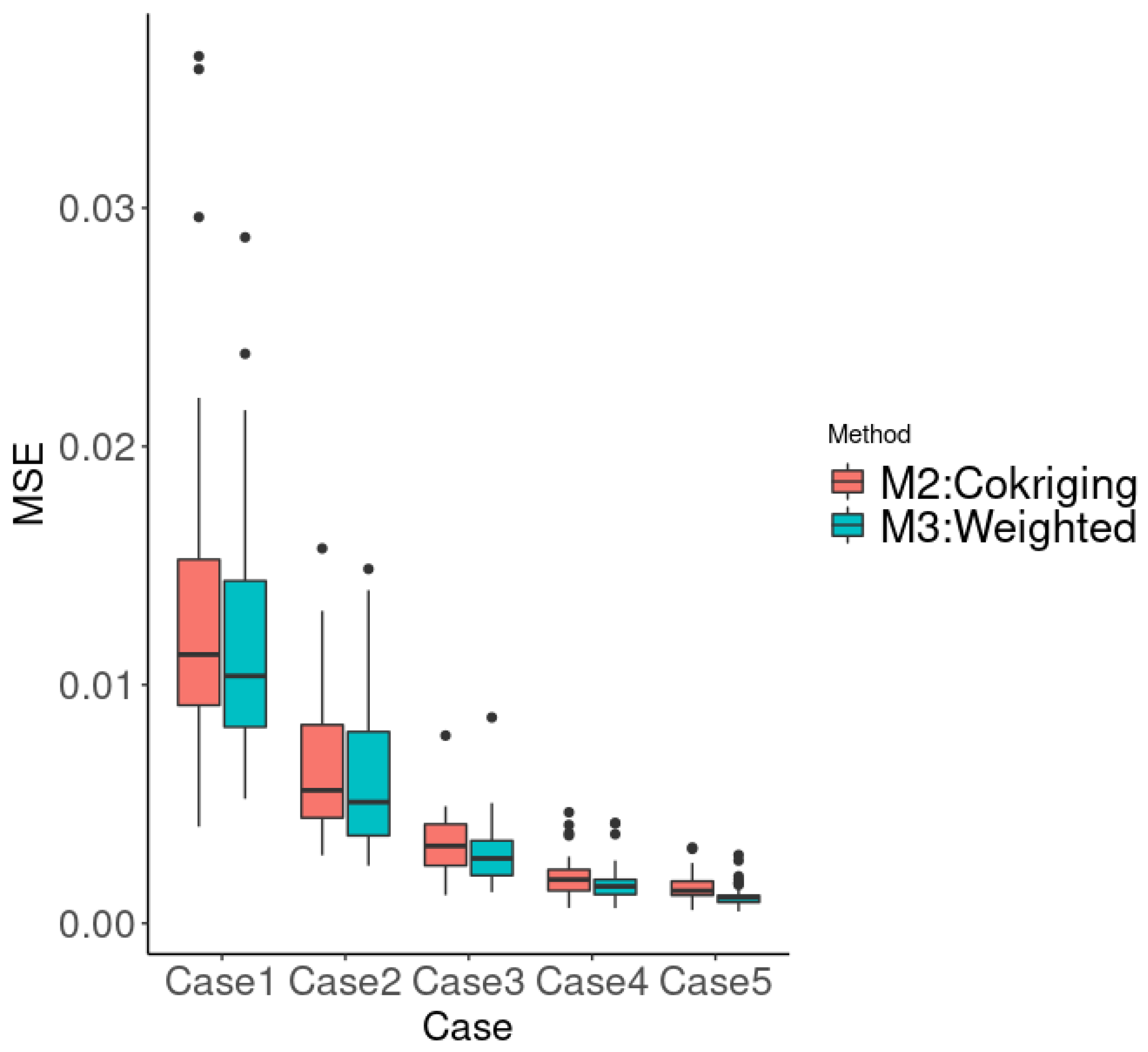
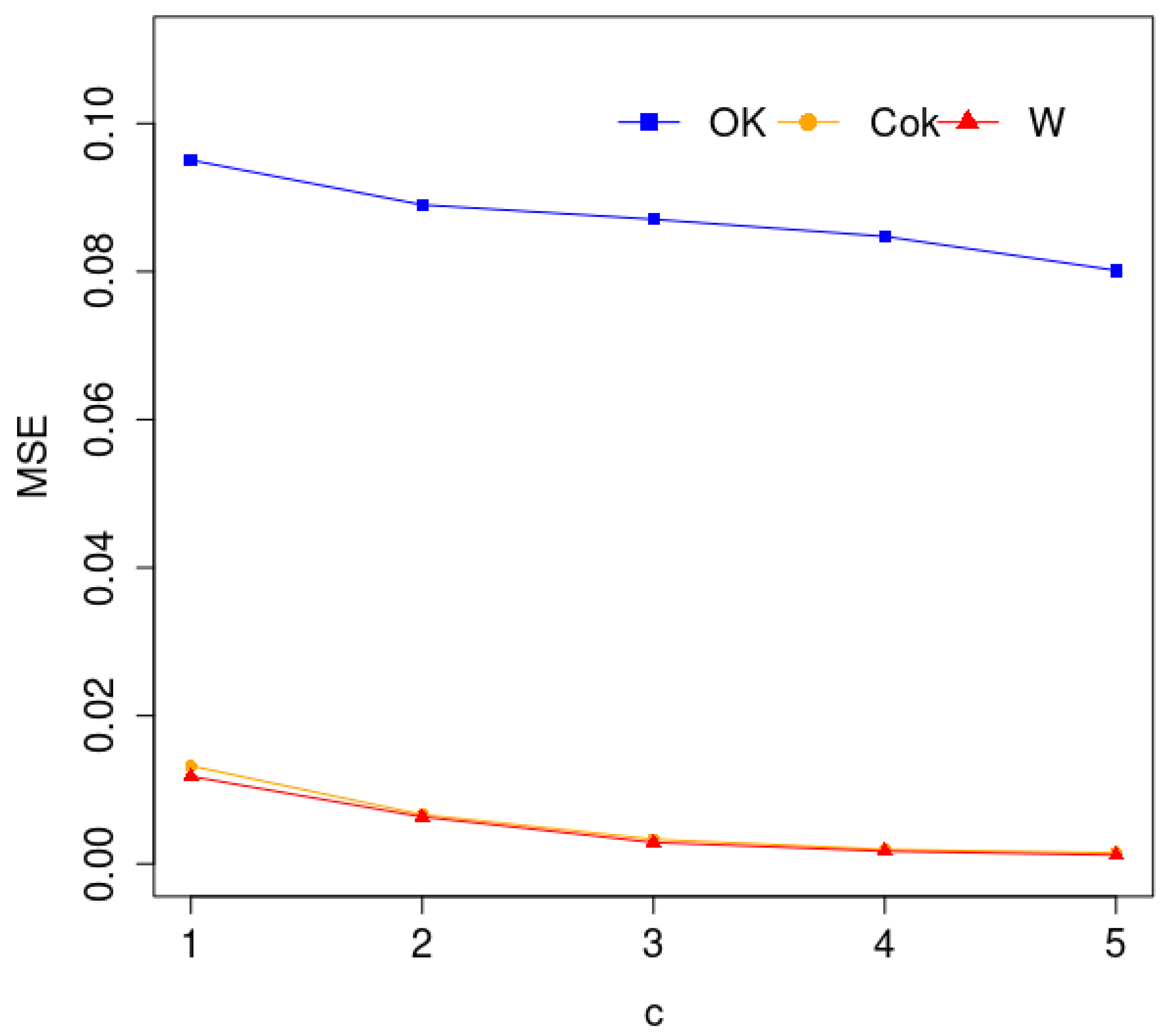
3. Simulation Studies

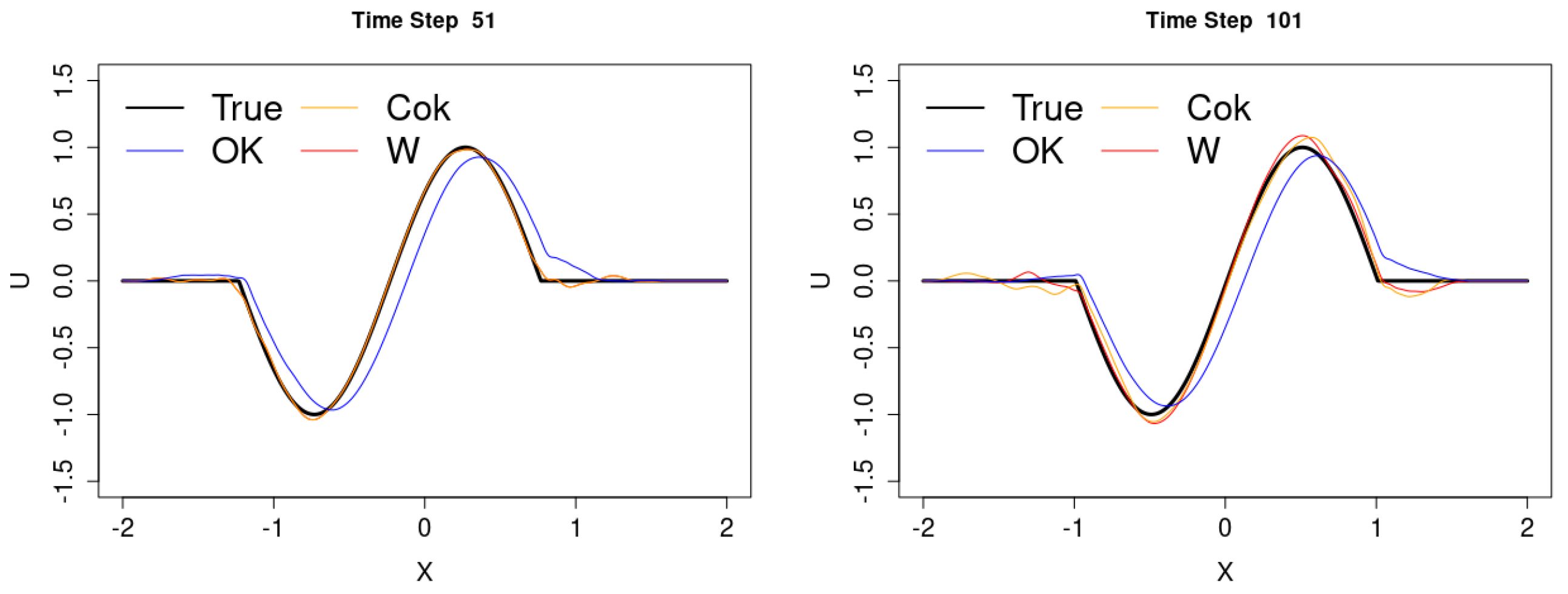
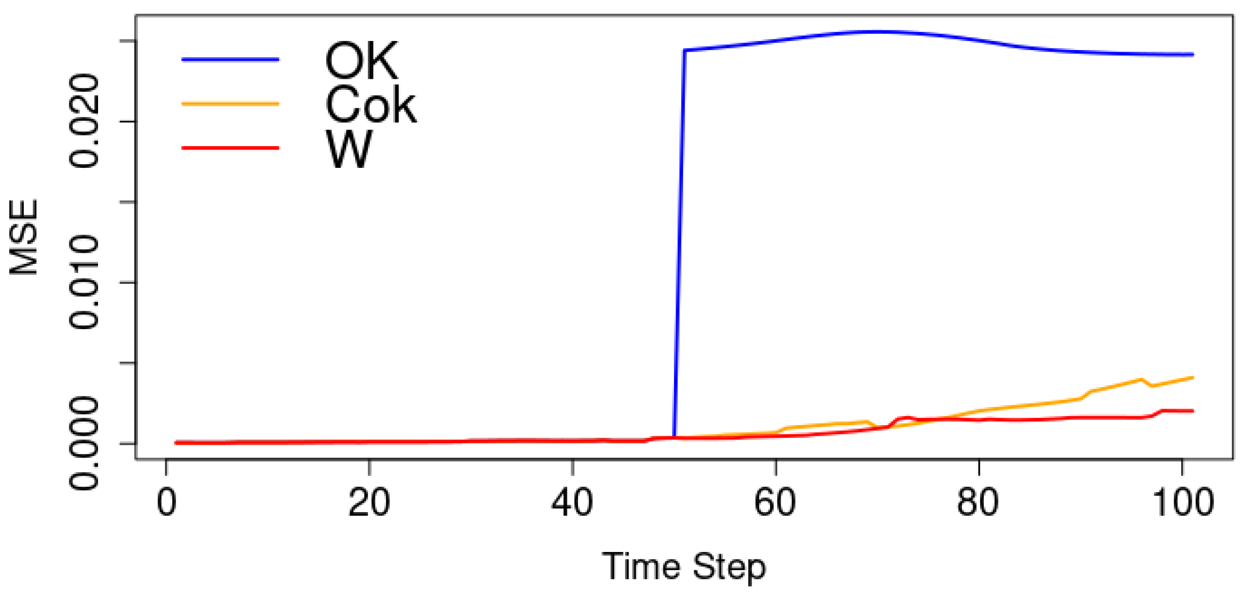
3.1. The Case of 2D Input Parameters for Spatio-Temporal Data

As a simple example, a one-dimensional advection equation is considered, with the initial phase ${\phi }_0$ and wave speed v as the input parameter. The advection equation represents a wave propagating with a constant velocity [21,22] of the form

$$\frac{\partial \mu }{\partial t}+v\frac{\partial \mu }{\partial x}=0,x\in [-2,2].$$

(16)

The initial condition is

$$\mu ={\mu }_0(x,0)=\{\begin{array}{c}0,\left|x\right|>1\\ Asin(\omega x+{\phi }_0),\left|x\right|⩽1\end{array},$$

(17)

and the boundary condition is

$$\mu (-2,t)=\mu (2,t).$$

(18)

Besides the input parameter $\theta ={({\phi }_0,v)}^T$, the above advection equation has two other control parameters, namely amplitude A and frequency $\omega$. We fixed the frequency $\omega =2\pi$ and amplitude $A=1$, and the input parameter space $\Omega =[0,1]\times [0,1]$. We take the space interval as $\Delta x=0.01$, and the time interval as $\Delta t=0.01$. The time range from 0 to 1 s is considered. Then, the spatio-temporal field is a grid of 401 space points and 101 time points. Let the interested time spans be ${\mathcal{T}}_1=\{0,0.01,0.02\cdots ,0.49\}$ and $\mathcal{T}={\mathcal{T}}_2=\{0,0.01,0.02\cdots ,0.99,1\}$. Our two proposed methods in Section 2.2.2 and in Section 2.2.3 are compared with the ordinary kriging method.

According to the reverse sequential sampling method proposed in Section 2.1, eight parameters were first sampled to form ${\Theta }_2$, and then, the other eight parameters were sampled to form ${\Theta }_1$. The parameters in $\Theta ={\Theta }_1\cup {\Theta }_2$ are listed in

Table 1. The training parameters.

$\mathit{\theta }$	${\mathit{\phi }}_0$	v	$\mathit{\theta }$	${\mathit{\phi }}_0$	v
${\theta }_{11}$	0.133	0.760	${\theta }_{21}$	0.176	0.662
${\theta }_{12}$	0.259	0.555	${\theta }_{22}$	0.688	0.186
${\theta }_{13}$	0.782	0.268	${\theta }_{23}$	0.951	0.338
${\theta }_{14}$	0.564	0.143	${\theta }_{24}$	0.405	0.891
${\theta }_{15}$	0.460	0.417	${\theta }_{25}$	0.327	0.456
${\theta }_{16}$	0.641	0.014	${\theta }_{26}$	0.043	0.608
${\theta }_{17}$	0.081	0.920	${\theta }_{27}$	0.820	0.079
${\theta }_{18}$	0.878	0.729	${\theta }_{28}$	0.545	0.975

. The spatio-temporal data at ${\mathcal{T}}_1$ were simulated under the parameters in $\Theta$, and the spatio-temporal data at ${\mathcal{T}}_2\setminus {\mathcal{T}}_1$ were simulated only under the input parameters in set ${\Theta }_2$. The training data were reduced by POD and the first 10 modes were chosen, which contain $99.21\%$ information of the training data. The time correlations of the time-varying coefficients of the first five modes are shown in Figure 2. Next, the surrogate models were built for ${\beta }_k(t_m,\theta )$, $m=1,2,\cdots ,101$, and $k=1,2,\cdots ,10$. We refer to the three schemes of establishing the surrogate model using the weighted method, cokriging method, and ordinary kriging methods as Schemes 1, 2, and 3, respectively.

Scheme 1: For $\beta (t_m;\theta )$, $t_m\in {\mathcal{T}}_1$, there were $|{\Theta }_1|+|{\Theta }_2|=16$ groups of training data, where $|·|$ means the element number of the set. The ordinary kriging models were established for $\beta (t_m;\theta )$ separately. For $\beta (t_m;\theta )$, $t_m\in {\mathcal{T}}_2\setminus {\mathcal{T}}_1$, there were only $|{\Theta }_2|=8$ groups of training data. Furthermore, the weighted method, which is proposed in Section 2.2.3, was used for $t_m\in {\mathcal{T}}_2\setminus {\mathcal{T}}_1$. $r_0$ is chosen as $0.7$.

Scheme 2: For $\beta (t_m;\theta )$, $t_m\in {\mathcal{T}}_1$, the model is the same as Scheme 1, and for $\beta (t_m;\theta )$, $t_m\in {\mathcal{T}}_2\setminus {\mathcal{T}}_1$, the cokriging method is used for ${\beta }_k(t,\theta )$ as introduced in Section 2.2.2.

Scheme 3: For $\beta (t_m;\theta )$, $t_m\in {\mathcal{T}}_2$, the ordinary kriging models are established separately.

The simulation results at ${\theta }_1^{*}={(0.483,0.427)}^T$ are chosen as the test data, which are used to evaluate the performance of the methods. For all three schemes, the predictions are given by (2). The predictions of the three methods for the spatio-temporal data under new parameters at $t_{51}=0.5$ s and $t_{101}=1.0$ s are shown in Figure 3. The predictions given by Schemes 1 and 2 are close to each other at $t_{51}$, and at $t_{101}$, and Scheme 1 is better than Scheme 2. Both Schemes 1 and 2 are significantly better than Scheme 3, which does not accurately capture the law of wave change. Figure 4 shows the prediction errors at each time step, defined as the average of the squared error of all spatial points. At $t_{51}$, the training parameters dropped from 16 to 8, which caused the prediction error of the ordinary kriging method to increase immediately, but both of our methods avoided the rapid increases because they used the information of the previous time steps. The weighted method includes the ordinary kriging method, which does not perform very well when the training data are reduced, but avoids predictions that deviate too far from the actual value when the data correlation weakens. In contrast with the cokriging method, the weighted method is therefore better in this example.

One simulation considers the effect of the number of input parameters, which is used to run further simulations. The details regarding the selection of parameters are shown in

Table 2. The number of input parameters in the simulations.

Case	Number
Case 1	$c_1=c_2=8$
Case 2	$c_1=c_2=10$
Case 3	$c_1=c_2=12$
Case 4	$c_1=c_2=14$
Case 5	$c_1=c_2=16$

. For each case, we randomly generated the training set and built the model 100 times, and for every trained surrogate model, 20 test parameters were sampled to verify the prediction error of the model.

The mean square error (MSE) is used as a metric to evaluate the performance of the method, which is defined as

$$MSE=\frac{1}{n_{te}·S·T}\sum _{i=1}^{n_{te}}\sum _{j=1}^S\sum _{k=1}^T{[f(x_j,t_k;\theta i)-\widehat{f}(x_j,t_k;\theta i)]}^2.$$

(19)

Figure 5 shows the boxplot of the MSE of our two proposed methods, and for different numbers of training samples, the weighted method is consistently better than the cokriging method; Figure 6 shows that the mean MSE of the three schemes varies with the amount of data, from which we can see that the MSE of the method we proposed is much smaller than that of the ordinary kriging method.

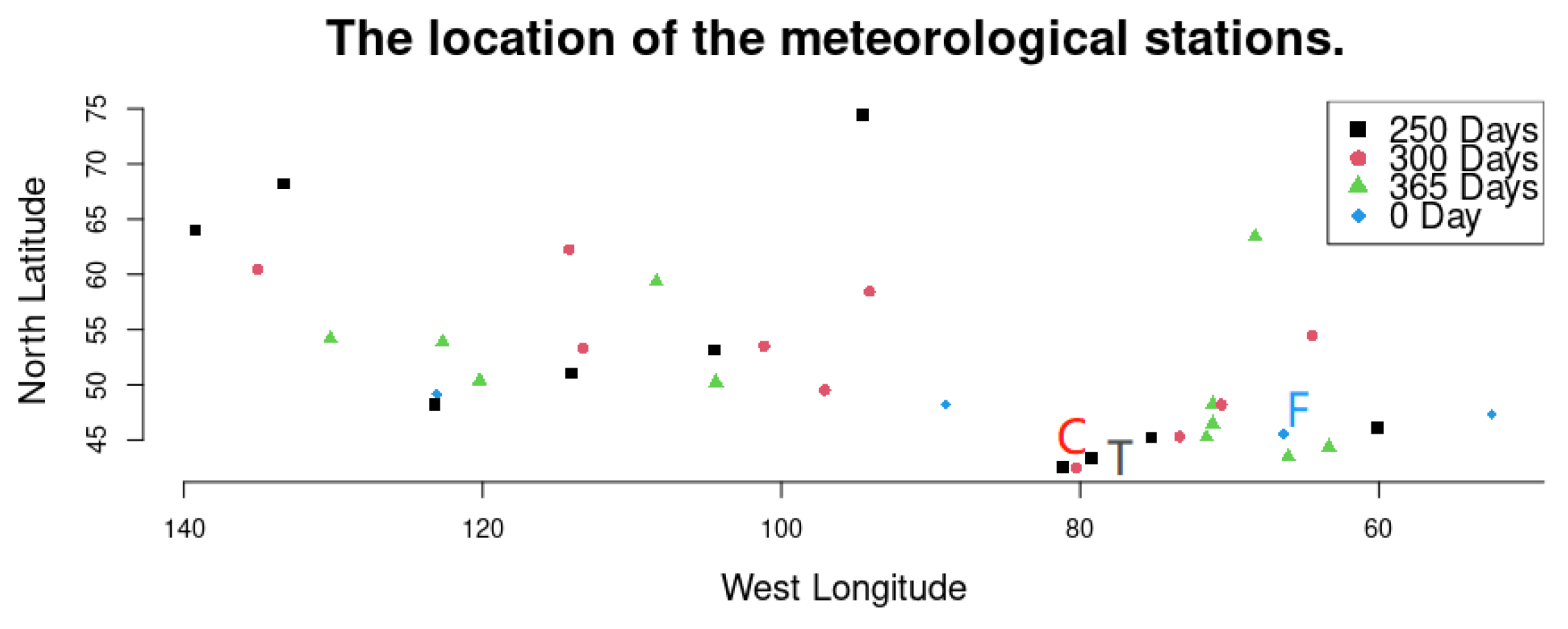
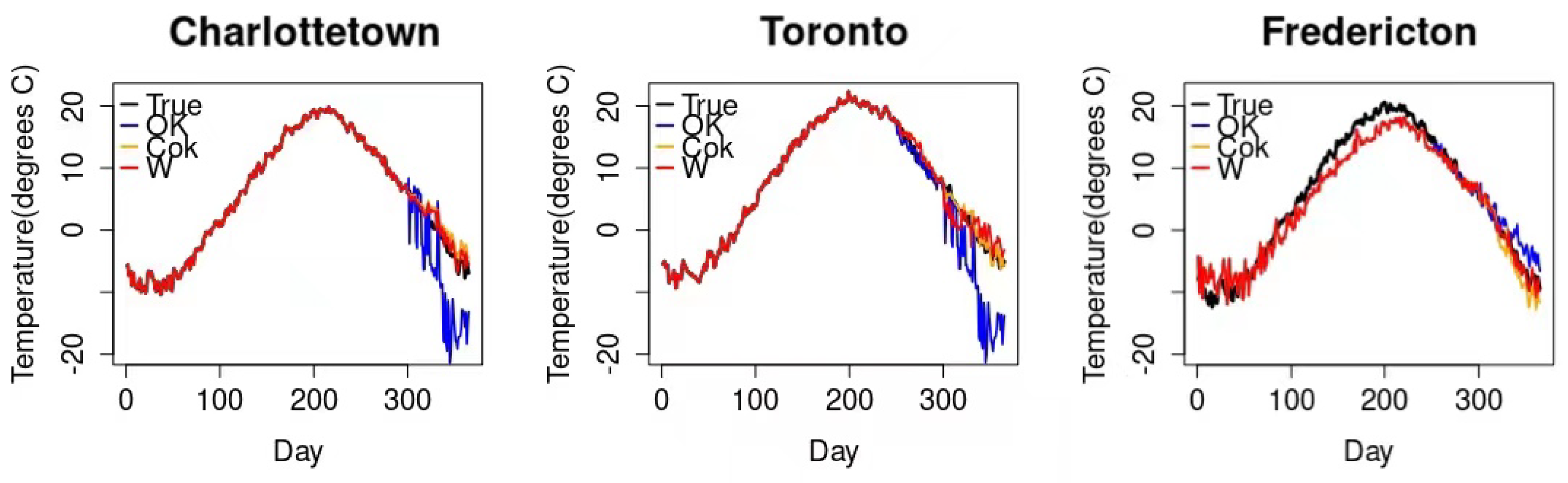
3.2. The Case of Canadian Weather

Our proposed methods are used for real observational spatio-temporal data. The R package fda provides Canadian weather data, including observations of daily temperature and precipitation at 35 different locations in Canada. Suppose that some of these stations have only the first 250 days of observations (represented by black squares in Figure 7), some have only the first 300 days of observations (represented by red circles in Figure 7), and some have all the observations (represented by green triangles in Figure 7). Furthermore, suppose that there are four stations without observational data that thus require prediction; these are considered the test data.

The stations at Charlottetown and Toronto were missing data for 65 days and 115 days, respectively, and the station at Fredericton had no observational data. We care about the prediction error for the time period when the data are missing. As a comparison, we built models using three methods, the ordinary kriging method, our proposed cokriging method, and our proposed weighted method. Figure 8 shows the real and forecast temperatures by the three methods at three weather stations. The two methods we proposed are significantly better than the ordinary kriging method. The MSE of the weighted method, cokriging method, and ordinary kriging method for the temperature of days 301 to 365 at the Charlottetown station are 1.454, 3.071, and 79.107, respectively. The MSE of the weighted method, cokriging method, and ordinary kriging method for the temperature of days 251 to 365 at the Toronto station are 3.263, 1.982, and 52.713, respectively. The MSE of the weighted method, cokriging method, and ordinary kriging method for the annual temperature at the Fredericton station are 3.361, 4.101, and 4.496, respectively.

In the example of the advection equation, the time correlation under some modes decreases very quickly—see Figure 2. In this situation, the weighted method performs better than the cokriging method. In the example of Canadian weather, the time correlation falls off more slowly relative to the advection equation example (Figure 9), and the cokriging method can also be used.

4. Application of the Model to Bai River Data

In this section, real data analysis for Bai River, which is located in Sichuan Province, as shown in Figure 10, is used to illustrate the performance of the proposed method. In the upper reaches of the river, there are some factory sewage pipes discharging a certain pollutant into the river. Assuming that there are two sewage outlets, A and B, then there are four-dimensional input parameters, the pollutant concentrations and water flow velocities of the two outlets, which are denoted as $\theta ={(p_A,p_B,v_A,v_B)}^T\in {[0,1]}^4$.

The simulator is the C++ code based on [23], which divides the geographic space into 37,960 mesh points. The time interval was $\Delta t=0.1$ s, and the solver was stored every 1000 steps. The solver with $M_2=1950$ time steps was calculated, which simulated the pollutant concentration in the Bai River over a 54 h period.

According to the reverse sequential sampling scheme, 10 parameters are selected for ${\Theta }_2$, and another 10 parameters are selected for ${\Theta }_1$, which is used to run the simulations. Suppose that when the simulation reached $t_{M_1},M_1=1000$, the detectors downstream of the river identified the high-level warning line of pollutants in the river. Thus, we needed to predict the change in pollutants in the future. However, we did not have enough time to simulate the spatio-temporal data under all parameters. Only the spatio-temporal data corresponding to the parameters in ${\Theta }_2$ were simulated, and a surrogate model was established in order to further judge which sewage outlet discharged pollutants excessively and caused the increase in pollution. The weighted method, cokriging method, and ordinary kriging method are used to establish the surrogate models. Figure 11 shows how pollutants at the red point and blue point in the Bai River map (Figure 10) changed over time. Figure 12 shows the prediction error of the three methods over the whole time span, which shows that two new methods are better than the original method.

5. Conclusions

Simulation is a common approach to the investigation of complex phenomena and systems. However, simulations are very expensive due to the requirement of solving large PDEs. How to best build surrogate models for simulations is an area still facing significant challenges. The goal of the surrogate models is to drastically reduce computational costs, especially when many predictions of spatio-temporal dynamics for unsimulated inputs are required. Most existing works in the literature only consider the situation with the same simulation time span. In this work, we consider the situation with multiple simulation time spans and propose a novel method to build efficient surrogate models. Firstly, a reverse sequential sampling method is presented to choose the input parameters for different simulation time spans. Then, a weighted surrogate model is proposed to fuse the spatio-temporal data from simulations with different time spans. The results of simulation studies and real data analysis based on Bai River in Sichuan Province of China show that the newly proposed method performs well and is superior to the traditional method.

The methods proposed in this work require that the spatio-temporal data are relatively smooth with respect to inputs and have correlations between time steps. The simulation studies also demonstrate that when the time correlations fall off quickly, the performance of the cokriging model deteriorates dramatically. Some random effects models could be considered to deal with this challenge, and will be studied in future work. The non-stationary nature of the data is another new challenge that will be considered.

References

1. Xiao, C.; Leeuwenburgh, O.; Lin, H.X.; Heemink, A. Non-intrusive subdomain POD-TPWL for reservoir history matching. Comput. Geosci. 2019, 23, 537–565. [Google Scholar] [CrossRef] [Green Version]
2. Lumley, J.L. The structure of inhomogeneous turbulent flows. In Atmospheric Turbulence and Radio Wave Propagation; NAUKA: Moscow, Russia, 1967; pp. 166–178. [Google Scholar]
3. Ioannidis, V.N.; Romero, D.; Giannakis, G.B. Inference of Spatio-Temporal Functions over Graphs via Multikernel Kriged Kalman Filtering. IEEE Trans. Signal Process. 2018, 66, 3228–3239. [Google Scholar] [CrossRef] [Green Version]
4. Nguyen, H.; Katzfuss, M.; Cressie, N.; Braverman, A. Spatio-temporal data fusion for very large remote sensing datasets. Technometrics 2014, 56, 174–185. [Google Scholar] [CrossRef]
5. Shi, Q.; Dai, W.; Santerre, R.; Liu, N. A Modified Spatiotemporal Mixed-Effects Model for Interpolating Missing Values in Spatiotemporal Observation Data Series. Math. Probl. Eng. 2020, 2020, 1070831. [Google Scholar] [CrossRef]
6. Guo, M.; Hesthaven, J.S. Data-driven reduced order modeling for time-dependent problems. Comput. Methods Appl. Mech. Eng. 2019, 345, 75–99. [Google Scholar] [CrossRef]
7. Yeh, S.T.; Wang, X.; Sung, C.L.; Mak, S.; Chang, Y.H.; Zhang, L.; Wu, C.F.; Yang, V. Common proper orthogonal decomposition-based spatiotemporal emulator for design exploration. AIAA J. 2018, 56, 2429–2442. [Google Scholar] [CrossRef] [Green Version]
8. Chang, Y.H.; Zhang, L.; Wang, X.; Yeh, S.T.; Mak, S.; Sung, C.L.; Jeff Wu, C.F.; Yang, V. Kernel-smoothed proper orthogonal decomposition-based emulation for spatiotemporally evolving flow dynamics prediction. AIAA J. 2019, 57, 5269–5280. [Google Scholar] [CrossRef]
9. Chang, Y.H.; Wang, X.; Zhang, L.; Li, Y.; Mak, S.; Wu, C.F.J.; Yang, V. Reduced-Order Modeling for Complex Flow Emulation by Common Kernel-Smoothed Proper Orthogonal Decomposition. AIAA J. 2021, 59, 3291–3303. [Google Scholar] [CrossRef]
10. Chatterjee, A. An introduction to the proper orthogonal decomposition. Curr. Sci. 2000, 78, 808–817. [Google Scholar]
11. Xiong, F.; Xiong, Y.; Chen, W.; Yang, S. Optimizing Latin hypercube design for sequential sampling of computer experiments. Eng. Optim. 2009, 41, 793–810. [Google Scholar] [CrossRef]
12. Garud, S.S.; Karimi, I.A.; Kraft, M. Design of computer experiments: A review. Comput. Chem. Eng. 2017, 106, 71–95. [Google Scholar] [CrossRef]
13. Joseph, V.R.; Gul, E.; Ba, S. Maximum projection designs for computer experiments. Biometrika 2015, 102, 371–380. [Google Scholar] [CrossRef]
14. Carnell, R.; Carnell, M.R. Package ‘lhs’. CRAN. Available online: http://cran.stat.auckland.ac.nz/web/packages/lhs/lhs.pdf (accessed on 22 March 2022).
15. Santner, T.J.; Williams, B.J.; Notz, W.I.; Williams, B.J. The Design and Analysis of Computer Experiments; Springer: New York, NY, USA, 2003; Volume 1. [Google Scholar]
16. Simpson, T.W.; Mauery, T.M.; Korte, J.J.; Mistree, F. Kriging models for global approximation in simulation-based multidisciplinary design optimization. AIAA J. 2001, 39, 2233–2241. [Google Scholar] [CrossRef] [Green Version]
17. Kleijnen, J.P. Kriging metamodeling in simulation: A review. Eur. J. Oper. Res. 2009, 192, 707–716. [Google Scholar] [CrossRef] [Green Version]
18. Vicario, G.; Craparotta, G.; Pistone, G. Meta-models in computer experiments: Kriging versus artificial neural networks. Qual. Reliab. Eng. Int. 2016, 32, 2055–2065. [Google Scholar] [CrossRef]
19. Kennedy, M.C.; O’Hagan, A. Predicting the output from a complex computer code when fast approximations are available. Biometrika 2000, 87, 1–13. [Google Scholar] [CrossRef] [Green Version]
20. Gratiet, L.L.; Garnier, J. Recursive co-kriging model for design of computer experiments with multiple levels of fidelity. Int. J. Uncertain. Quantif. 2014, 4, 365–386. [Google Scholar] [CrossRef]
21. Hu, F.Q.; Hussaini, M.Y.; Rasetarinera, P. An analysis of the discontinuous Galerkin method for wave propagation problems. J. Comput. Phys. 1999, 151, 921–946. [Google Scholar] [CrossRef]
22. Vadyala, S.R.; Betgeri, S.N.; Betgeri, N.P. Physics-informed neural network method for solving one-dimensional advection equation using PyTorch. Array 2022, 13, 100110. [Google Scholar] [CrossRef]
23. Shen, H.; Parsani, M. Positivity-preserving CE/SE schemes for solving the compressible Euler and Navier–Stokes equations on hybrid unstructured meshes. Comput. Phys. Commun. 2018, 232, 165–176. [Google Scholar] [CrossRef]
Figure 1. An illustration of the reverse sequential sampling scheme.
Mathematics 10 03585 g001
Figure 2. Time correlations of the time-varying coefficient corresponding to the first five POD modes in the advection equation example.
Mathematics 10 03585 g002
Figure 3. The left and right panels show the true and predicted waves at t 51 = 0.5 s and t 101 = 1.0 s, respectively. The black lines are the true data, and the red, orange, and blue lines are the predictions given by Schemes 1, 2, and 3, respectively.
Mathematics 10 03585 g003
Figure 4. The prediction errors at each time step.
Mathematics 10 03585 g004
Figure 5. The MSE of our two proposed methods.
Mathematics 10 03585 g005
Figure 6. The mean MSE of the three schemes varies with the amount of data.
Mathematics 10 03585 g006
Figure 7. The location of 35 weather stations. C, T, and F represent the locations of Charlottetown, Toronto, and Fredericton, respectively.
Mathematics 10 03585 g007
Figure 8. Predictions of Canadian weather.
Mathematics 10 03585 g008
Figure 9. Time correlations of temperature in the Canadian weather example.
Mathematics 10 03585 g009
Figure 10. The shape of the Bai River.
Mathematics 10 03585 g010
Figure 11. Changes in pollutants at one point in the Bai River over the whole time span.
Mathematics 10 03585 g011
Figure 12. The MSE at each time step.
Mathematics 10 03585 g012