Accelerating Extreme Search of Multidimensional Functions Based on Natural Gradient Descent with Dirichlet Distributions

Abstract

The high accuracy attainment, using less complex architectures of neural networks, remains one of the most important problems in machine learning. In many studies, increasing the quality of recognition and prediction is obtained by extending neural networks with usual or special neurons, which significantly increases the time of training. However, engaging an optimization algorithm, which gives us a value of the loss function in the neighborhood of global minimum, can reduce the number of layers and epochs. In this work, we explore the extreme searching of multidimensional functions by proposed natural gradient descent based on Dirichlet and generalized Dirichlet distributions. The natural gradient is based on describing a multidimensional surface with probability distributions, which allows us to reduce the change in the accuracy of gradient and step size. The proposed algorithm is equipped with step-size adaptation, which allows it to obtain higher accuracy, taking a small number of iterations in the process of minimization, compared with the usual gradient descent and adaptive moment estimate. We provide experiments on test functions in four- and three-dimensional spaces, where natural gradient descent proves its ability to converge in the neighborhood of global minimum. Such an approach can find its application in minimizing the loss function in various types of neural networks, such as convolution, recurrent, spiking and quantum networks.

1. Introduction

The optimization methods remain the most important and critical problems in artificial neural networks, which significantly impact the process of recognition. They allow us to solve many problems approximately, without a complex analytical approach. The most usable optimization algorithm in machine learning is stochastic gradient descent and its modified versions, which include momentum and the Nesterov condition. Afterwards, for increasing the accuracy, there were proposed AdaGrad in [1,2], RMSprop in [3] and ADADELTA and the Adam algorithm in [4,5], respectively. However, they are not rapid enough and, usually, converge to the local extreme. Even step-size adaptation from [6] cannot achieve the desired accuracy, reducing the number of iterations. The most appropriate solution in this case is researching the optimization of the loss function using the means of Riemannian geometry.

The metric properties are described in Riemannian geometry on arbitrary n-dimensional smooth manifolds with local coordinates. According to the type of manifold, we can provide the gradient flow that improves the quality of the optimization process. The gradient flow from [7] is the product between the metric tensor and gradient of the optimizing function. Such an approach in optimization accelerates the convergence and minimizes iterations (epochs). However, in this manuscript, we provide the extreme search with manifolds of probability distributions.

Probability distribution manifolds mostly can be found in information geometry, where the analog of gradient flow is the natural gradient. The analog of the metric tensor is the Fisher information matrix, which depends on some probability distribution. The Fisher matrix is calculated by the Kullback–Leibler divergence (K–L divergence in [8,9,10]). Taking into account the convexity of the optimizing function, it is possible to increase the accuracy without changing the initial step size and numerical value of the gradient.

Natural gradient descent (NGD) is an alternative to stochastic gradient descent and its modifications, as was noted in [11]. Unfortunately, for models with many parameters, such as convolution neural networks, computing the natural gradient in every iteration is ineffective because of the extremely large size of the Fisher matrix. This problem can be solved using various approximations to the Fisher matrix, as in [12,13]. It is designed to facilitate the computation, storing and finally inversion of the exact Fisher matrix. Moreover, it is possible to reduce the computations by applying a proper probability distribution.

In this article, we propose the algorithm of natural gradient descent with step-size adaptation based on Dirichlet and generalized Dirichlet distributions. We demonstrate that the natural gradient descent with step-size adaptation based on Dirichlet and generalized Dirichlet distributions has higher accuracy and does not take a large number of iterations for minimizing test functions compared to gradient descent and Adam. Such an approach is a continuation of works [14,15], where the final results did not present the ability of natural gradient descent to converge in the neighborhood of the global minimum.

The remainder of the paper is organized as follows. Section 2 presents the background of gradient descent, Adam and gradient flow. Section 3 contains calculations of the Fisher information matrices of Dirichlet and generalized Dirichlet distributions and proposes the algorithms of natural gradient descent based on Dirichlet and generalized Dirichlet distributions. Section 4 consists of experiments on the minimization of test functions with corresponding graphs and tables. In Section 5, we report the conclusions of the obtained results and suggestions for improving the natural gradient descent and its further exploitation in neural networks.

2. Preliminaries

2.1. Gradient Descent with Step-Size Adaptation

Let us consider a continuous function $f:\mathsf{\Omega }\to \mathbb{R}$, defined on closed convex domain $\mathsf{\Omega }\in \mathbb{R}$. The main goal of minimization is finding ${min}_{x\in \mathsf{\Omega }}f(x)$.

This is a necessary process for achieving the high accuracy of predictions in every artificial neural network, due to the more rapid and exact minimization of loss functions. The gradient descent, presented in Algorithm 1, with appropriate step-size adaptation in [6] has advantages in rate and accuracy over stochastic gradient descent.

Note that, in general cases, gradient descent cannot reach the minimum, because of the constant steps and confusion of the gradient in cases of several local extremes. Performing step-size adaptation does not guarantee descent into the global minimum, due to the large number of local minima. However, it allows us to increase the accuracy. This problem led the researchers to replace this method with Adam.

Algorithm 1 Gradient Descent with Step-Size Adaptation

Input:  $x_0\in {\mathbb{R}}^n$ (starting point), f (scalar function), $\nabla f$ (gradient), $a_0$ (initial step size), n (number of iterations) Output:  some $x_n$ minimizing f 1: initialize $f_0=f(x_0)\in \mathbb{R}$, $g_0=\nabla f{(x_0)}^T\in {\mathbb{R}}^n$ 2: for i from 1 to n do 3:   $x_i\leftarrow x_{i-1}-a_0{g}_{i-1}/\left|g_{i-1}\right|$ 4:   $f_i\leftarrow f(x_i)$ 5:   if $f_i<f_{i-1}$ then 6:    $f_i\leftarrow f_{i-1}$ 7:    $a_i\leftarrow 1.2a_{i-1}$ 8:   else 9:    $a_i\leftarrow 0.5a_{i-1}$ 10:  end if 11:  $g_i\leftarrow \nabla f{(x_i)}^T$ 12: end for

2.2. Adam Algorithm

The Adam algorithm [5] is an attempt to improve the stochastic gradient descent, which updates the exponential moving averages of the gradient $m_t$ and the squared gradient $v_t$ with the hyper-parameters ${\beta }_1,{\beta }_2\in [0,1)$ to control the exponential decay rates of these moving averages. The moving averages themselves are estimates of the first moment (the mean) and the second raw moment (the uncentered variance) of the gradient. However, these moving averages are initialized as (vectors of) 0 s, leading to moment estimates that are biased towards zero, especially during the initial time steps, and especially when the decay rates are small. The advantage is that this initialization bias can be easily counteracted, resulting in bias-corrected estimates ${\widehat{m}}_t$ and ${\widehat{v}}_t$. The step-size adaptation improves the quality of the Adam algorithm, which means accelerating the minimization and increasing the accuracy. These amendments can be helpful in deep neural networks because the optimizer gives more accurate results in less time.

Let us present the pseudo-code of the Adam method in Algorithm 2.

Algorithm 2 Adam algorithm

Input:  $x_0\in {\mathbb{R}}^n$ (starting point), f (scalar function), $\nabla f$ (gradient), $a_0$ (initial step size), n (number of iterations), ${\beta }_1$, ${\beta }_2$ (exponential decay rates) Output:  some $x_n$ minimizing f 1: initialize $f_0=f(x_0)\in \mathbb{R}$, $g_0=\nabla f_0^T\in {\mathbb{R}}^n$, $m_0=0$, $v_0=0$ 2: for i from 1 to n do 3:   $m_i\leftarrow {\beta }_1{m}_{i-1}+(1-{\beta }_1)g_{i-1}$ 4:   $v_i\leftarrow {\beta }_2{v}_{i-1}+(1-{\beta }_2)g_{i-1}^2$ 5:   ${\widehat{m}}_i\leftarrow m_i/(1-{\beta }_1^i)$ 6:   ${\widehat{v}}_i\leftarrow v_i/(1-{\beta }_1^i)$ 7:   $x_i\leftarrow x_{i-1}-a_{i-1}·{\widehat{m}}_i/(\sqrt{\widehat{v_i}}+ϵ)$ 8:   $f_i\leftarrow f(x_i)$ 9:   if $f_i<f_{i-1}$ then 10:   $f_i\leftarrow f_{i-1}$ 11:   $a_i\leftarrow 1.2a_{i-1}$ 12:  else 13:   $a_i\leftarrow 0.5a_{i-1}$ 14:  end if 15:  $g_i\leftarrow \nabla f(x_i)$ 16: end for

In the process of learning neural networks, the Adam algorithm is the most preferred optimization method, because it converges faster and gives the required accuracy. However, this algorithm does not contain the curvature of the function $n-1$-surfaces, for $n\ge 2$. Therefore, it does not reach the global minimum for small steps in the case of very convex functions such as Rastrigin, which is shown in Section 4.2.

2.3. Background on Riemannian Gradient Flow

The main idea of natural gradient descent initially comes from Riemannian geometry, where the definitions of derivative, flow and curvature are generally described.

We denote $(M,g)$ as a Riemannian manifold, where $M={\mathbb{R}}^n$ is the topological space and $g:M\times M\to \mathbb{R}$ is the metric tensor. The tangent space $T_x$, where $T_{x}M={\mathbb{R}}^n$, and the metric tensors $g(x)\in {\mathbb{S}}_{++}^n$, where ${\mathbb{S}}_{++}^n$ is the cone of real symmetric definite positive matrices [16], can be taken for manifold M. The tensor matrix $g(x,x+\delta x)$ defines the local distances at x as $d{(x,x+\delta x)}^2=\delta x^{T}g(x,\delta x)\delta x$ for $\delta x\to \infty$. The following gradient vector field of the minimizing function f restricted to $\mathsf{\Omega }$ [16] is denoted as

$${\nabla }_{g}f{\mid }_{\mathsf{\Omega }}=g{(x,x+\delta x)}^{-1}\nabla f(x).$$

(1)

The information geometry [17] is a manifold of probability distributions, e.g., a parametric family $p(x;\theta ):\theta \in {\mathbb{R}}^n$, endowed with the metric, which is derived from the Kullback–Leibler divergence formula. The natural gradient is defined on such manifolds.

2.4. Natural Gradient Descent and K–L Divergence

NGD in [11] is obtained as the forward Euler discretization with step size $\eta$ of the gradient flow (1):

$$x^{(k+1)}=x^{(k)}-{\eta }_{k}F{(x^{(k)})}^{-1}\nabla f(x^{(k)}),$$

(2)

where $x^{(0)}=x_0$.

The Fisher information matrix $F(x^{(k)})$ from [11,14,17] can be calculated on the manifold of probability distributions, whose curvature we use to minimize the continuous function $f(\theta )$. Presume that $p(x;\theta )$ is a family of probability distributions over space variables x with a parametric vector $\theta \in {\mathbb{R}}^n$. Let us introduce the K–L divergence.

$$\begin{array}{c}KL(p(x;{\theta }_t)\left|\right|p(x;{\theta }_t+\delta \theta ))=\int p(x;{\theta }_t)log\frac{p(x;{\theta }_t)}{p(x;{\theta }_t+\delta \theta )}dx\\ =\int p(x;{\theta }_t)logp(x;{\theta }_t)dx-\int p(x;{\theta }_t)logp(x;{\theta }_t+\delta \theta )dx.\end{array}$$

(3)

Next, we provide the second Taylor series expansion of the function f as

$$f(\theta )\approx f({\theta }_t)+\nabla f{({\theta }_t)}^T\delta \theta +\frac{1}{2}\delta {\theta }^T{\nabla }^{2}f({\theta }_t)\delta \theta ,$$

(4)

where $\theta ={\theta }_t+\delta \theta$, and ${\nabla }^{2}f$ is a Hessian matrix.

Substituting (3) into (4), we obtain

$$\begin{array}{c}KL(p(x;{\theta }_t)\left|\right|p(x;{\theta }_t+\delta \theta ))\approx \int p(x;{\theta }_t)logp(x;{\theta }_t)dx\\ =\int p(x;{\theta }_t)log\frac{p(x;{\theta }_t)}{p(x;{\theta }_t)}dx-{\left(\int \nabla p(x;{\theta }_t)dx\right)}^T\delta \theta -\frac{1}{2}\delta {\theta }^T\left(\int p(x;{\theta }_t){\nabla }^{2}logp(x;{\theta }_t)dx\right)\delta \theta .\end{array}$$

The first two integrals are equal to 0, because $log\frac{p(x;{\theta }_t)}{p(x;{\theta }_t)}=log1=0$ and

$$\int \nabla p(x;{\theta }_t)dx=\nabla \int p(x;{\theta }_t)dx=\nabla 1=0.$$

Therefore, we obtain K–L divergence for probability distribution $p(x;{\theta }_t)$:

$$KL(p(x;{\theta }_t)\left|\right|p(x;{\theta }_t+\delta \theta ))\approx \frac{1}{2}\delta {\theta }^T\left(\int p(x;{\theta }_t){\nabla }^{2}logp(x;{\theta }_t)dx\right)\delta \theta .$$

Let us provide the Hessian ${\nabla }^{2}logp(x;{\theta }_t)$, which can be split into two products:

$${\nabla }^{2}logp(x;{\theta }_t)=\nabla logp(x;{\theta }_t)\nabla logp(x;{\theta }_t){)}^T.$$

Then, the K–L divergence has the following form:

$$\begin{array}{c}KL(p(x;{\theta }_t)||p(x;{\theta }_t+\delta \theta ))\\ =-\frac{1}{2}\delta {\theta }^T\mathbb{E}\left[\nabla logp(x;{\theta }_t)\nabla log{p(x;{\theta }_t)}^T\right]\delta \theta =-\frac{1}{2}\delta {\theta }^{T}F({\theta }_t)\delta \theta ,\end{array}$$

(5)

where $F({\theta }_t)$ is a Fisher information matrix, which is a Riemannian structure on a manifold of probability distributions.

3. Theoretical Calculations

Fisher Matrix for Dirichlet and Generalized Dirichlet Distributions

The Dirichlet distribution of order $K\ge 2$ with parameters ${\alpha }_1,\dots ,{\alpha }_K>0$ [18] has a probability density function with respect to the Lebesgue measure on the Euclidean space ${\mathbb{R}}^{K-1}$ given by

$$\begin{array}{c}\hfill p(x_1,\dots ,x_K;{\alpha }_1,\dots ,{\alpha }_K)=\frac{1}{B(\alpha )}\prod _{i=1}^K{x}_i^{{\alpha }_i-1},B(\alpha )=\frac{{\prod }_i\mathsf{\Gamma }({\alpha }_i)}{\mathsf{\Gamma }({\sum }_i{\alpha }_i)},\end{array}$$

(6)

where ${\left\{x_i\right\}}_{i=1}^K$ belongs to the $K-1$ simplex.

Let us calculate the logarithm of Dirichlet distribution:

$$\begin{array}{c}\hfill logp(x_1,\dots ,x_K;{\alpha }_1,\dots ,{\alpha }_K)=log\left[\frac{\mathsf{\Gamma }({\sum }_i{\alpha }_i)}{{\prod }_i\mathsf{\Gamma }({\alpha }_i)}\prod _{i=1}^K{x}_i^{{\alpha }_i-1}\right]\\ \hfill =log\mathsf{\Gamma }(\sum _{i=1}^K{\alpha }_i)-\sum _{i=1}^{K}log\mathsf{\Gamma }({\alpha }_i)+\sum _{i=1}^K({\alpha }_i-1)log{x}_i.\end{array}$$

Afterwards, we imply the second-order partial derivative of f with respect to $\alpha$ and obtain

$$\frac{{\partial }^2}{\partial a_j\partial a_k}logp={\psi }^{\prime }\left(\sum _{i=1}^K{\alpha }_i\right),\frac{{\partial }^2}{\partial a_j^2}logp={\psi }^{\prime }\left(\sum _{i=1}^K{\alpha }_i\right)-{\psi }^{\prime }({\alpha }_j).$$

Hence, we have the Fisher information matrix of Dirichlet distribution:

$$\begin{array}{c}\hfill F_{Dir}(\alpha )=\left(\begin{array}{ccc}{\psi }^{\prime }({\alpha }_1)-{\psi }^{\prime }(\sum _i{\alpha }_i)& \dots & -{\psi }^{\prime }(\sum _i{\alpha }_i)\\ \dots & \dots & \dots \\ -{\psi }^{\prime }(\sum _i{\alpha }_i)& \dots & {\psi }^{\prime }({\alpha }_K)-{\psi }^{\prime }(\sum _i{\alpha }_i)\end{array}\right).\end{array}$$

(7)

The generalized Dirichlet distribution [18] for $x_1+\dots +x_K\le 1$ and ${\alpha }_i>0,{\beta }_i>0,i=1,\dots ,K-1$ has a probability density function, which is defined as

$$\begin{array}{c}\hfill p(x_1,\dots ,x_K;{\alpha }_1,\dots ,{\alpha }_K,{\beta }_1,\dots ,{\beta }_K)=\prod _{i=1}^K\frac{1}{B({\alpha }_i,{\beta }_i)}{x}_i^{{\alpha }_i-1}{\left(1-\sum _{j=1}^i{x}_j\right)}^{{\gamma }_i},\end{array}$$

(8)

where ${\gamma }_i={\beta }_i-{\alpha }_{i+1}-{\beta }_{i+1}$ for $i=1,\dots ,K-1$ and ${\gamma }_K={\beta }_{K-1}$.

The logarithm (7) is

$$\begin{array}{c}\hfill logp=log\left[\prod _{i=1}^K\frac{\mathsf{\Gamma }({\alpha }_i+{\beta }_i)}{\mathsf{\Gamma }({\alpha }_i)\mathsf{\Gamma }({\beta }_i)}{x}_i^{{\alpha }_i-1}{\left(1-\sum _{j=1}^i{x}_j\right)}^{{\gamma }_i}\right]=\sum _{i=1}^{K}log\mathsf{\Gamma }({\alpha }_i+{\beta }_i)\\ \hfill -\sum _{i=1}^{K}log\mathsf{\Gamma }({\alpha }_i)-\sum _{i=1}^{K}log\mathsf{\Gamma }({\beta }_i)+\sum _{i=1}^K({\alpha }_i-1)log{x}_i+\sum _{i=1}^K{\gamma }_{i}log(1-\sum _{j=1}^i{x}_j).\end{array}$$

The second-order partial derivatives of $logf(x;\alpha ,\beta )$ are

$$\begin{array}{c}\hfill (1)\frac{{\partial }^2}{\partial {\alpha }_j\partial {\alpha }_l}logp=\frac{{\partial }^2}{\partial {\beta }_j\partial {\beta }_l}logp=\frac{{\partial }^2}{\partial {\alpha }_j\partial {\beta }_l}logp=0,j\ne l,\\ \hfill (2)\frac{{\partial }^2}{\partial {\alpha }_j^2}logp={\psi }^{\prime }({\alpha }_j+{\beta }_j)-{\psi }^{\prime }({\alpha }_j),\frac{{\partial }^2}{\partial {\beta }_j^2}logp={\psi }^{\prime }({\alpha }_j+{\beta }_j)-{\psi }^{\prime }({\beta }_j),\\ \hfill (3)\frac{{\partial }^2}{\partial {\alpha }_j\partial {\beta }_j}logp=\frac{{\partial }^2}{\partial {\beta }_j\partial {\alpha }_j}logp={\psi }^{\prime }({\alpha }_j+{\beta }_j).\end{array}$$

Then, the Fisher matrix for the generalized Dirichlet distribution has the following form:

$$\begin{array}{c}\hfill F_{GenDir}(\alpha )=\left(\begin{array}{cccc}{\mathsf{\Psi }}_1& \mathcal{O}& \dots & \mathcal{O}\\ \mathcal{O}& {\mathsf{\Psi }}_2& \dots & \dots \\ \dots & \dots & \dots & \dots \\ \mathcal{O}& \dots & \mathcal{O}& {\mathsf{\Psi }}_K\end{array}\right),\end{array}$$

(9)

where

$$\begin{array}{c}\hfill {\mathsf{\Psi }}_i=\left(\begin{array}{cc}{\psi }^{\prime }({\alpha }_i)-{\psi }^{\prime }({\alpha }_i+{\beta }_i)& -{\psi }^{\prime }({\alpha }_i+{\beta }_i)\\ -{\psi }^{\prime }({\alpha }_i+{\beta }_i)& {\psi }^{\prime }({\beta }_i)-{\psi }^{\prime }({\alpha }_i+{\beta }_i)\end{array}\right)and\mathcal{O}isazeromatrix.\end{array}$$

According to the Fisher information matrix for Dirichlet and generalized Dirichlet distributions, and adding the step-size adaptation, we propose Algorithm 3.

Algorithm 3 Natural Gradient Descent with Dirichlet and Generalized Dirichlet Distribution

Input:  $x_0\in {\mathbb{R}}^n$ (starting point), f (scalar function), $\nabla f$ (gradient), $a_0$ (initial step size), n (number of iterations) Output:  some $x_n$ minimizing f 1: initialize $f_0=f(x_0)\in \mathbb{R}$, $g_0=\nabla f{(x_0)}^T\in {\mathbb{R}}^n$ and Fisher matrix F 2: for i from 1 to n do 3:   $x_i\leftarrow x_{i-1}-a_{i-1}{F}^{-1}{g}_{i-1}/\left|g_{i-1}\right|$ 4:   $f_i\leftarrow f(x_i)$ 5:   if $f_i<f_{i-1}$ then 6:    $f_i\leftarrow f_{i-1}$ 7:    $a_i\leftarrow 1.2a_{i-1}$ 8:   else 9:    $a_i\leftarrow 0.5a_{i-1}$ 10:  end if 11:  $g_i\leftarrow \nabla f{(x_i)}^T$ 12: end for

Note that, in Algorithm 3, it is unnecessary to reduce the length of steps or the numerical value of the gradient to improve the final values of extremes. The Fisher matrix contains parameters without items of vector x, which allows us to avoid additional computations in the loop. Including curvature properties by the Fisher matrix natural gradient achieves extremes faster. Finally, the Fisher information matrix with generalized Dirichlet distribution is useful only in cases of 2n-dimensional surfaces, where $n\in \mathbb{N}$.

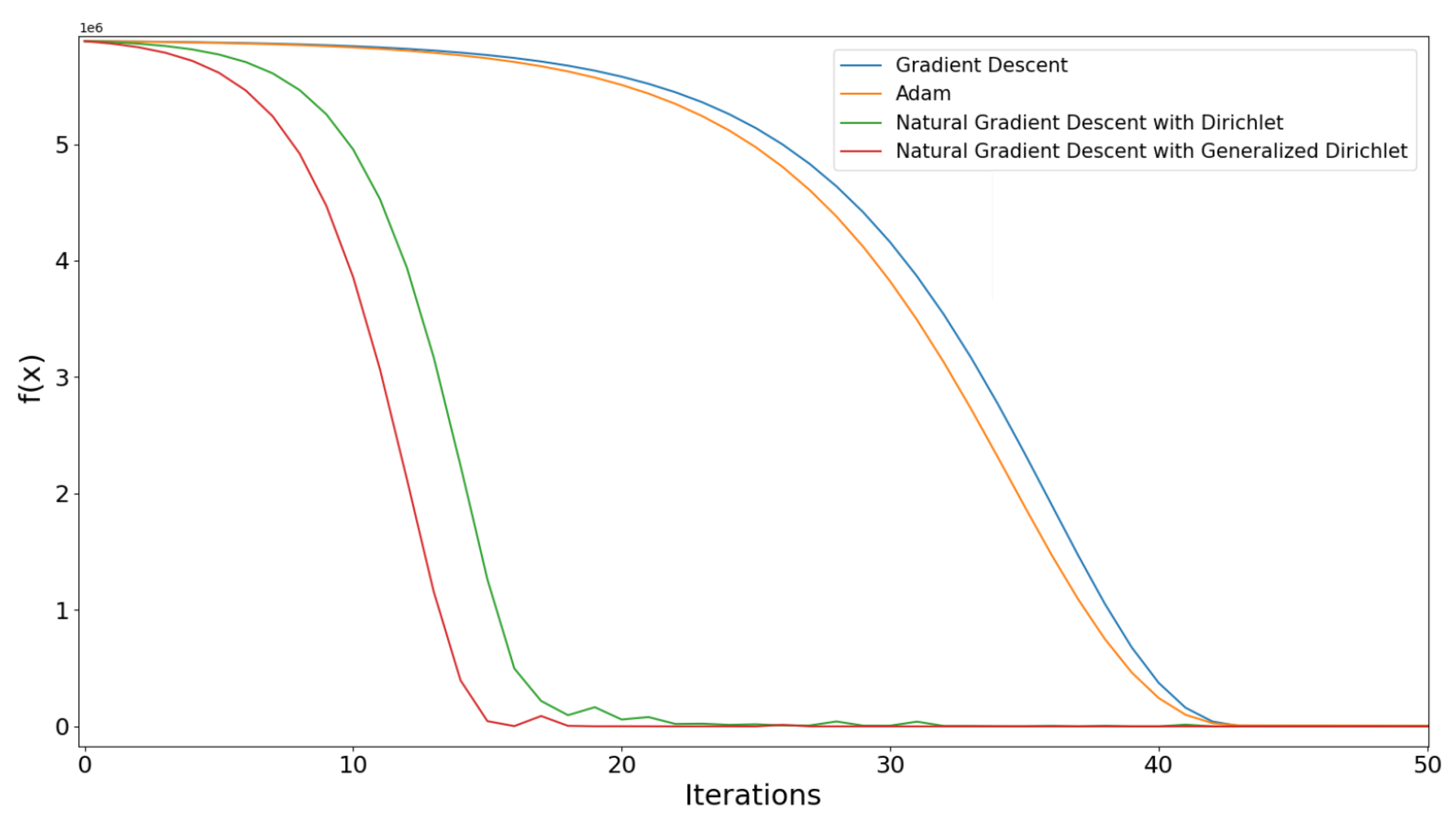
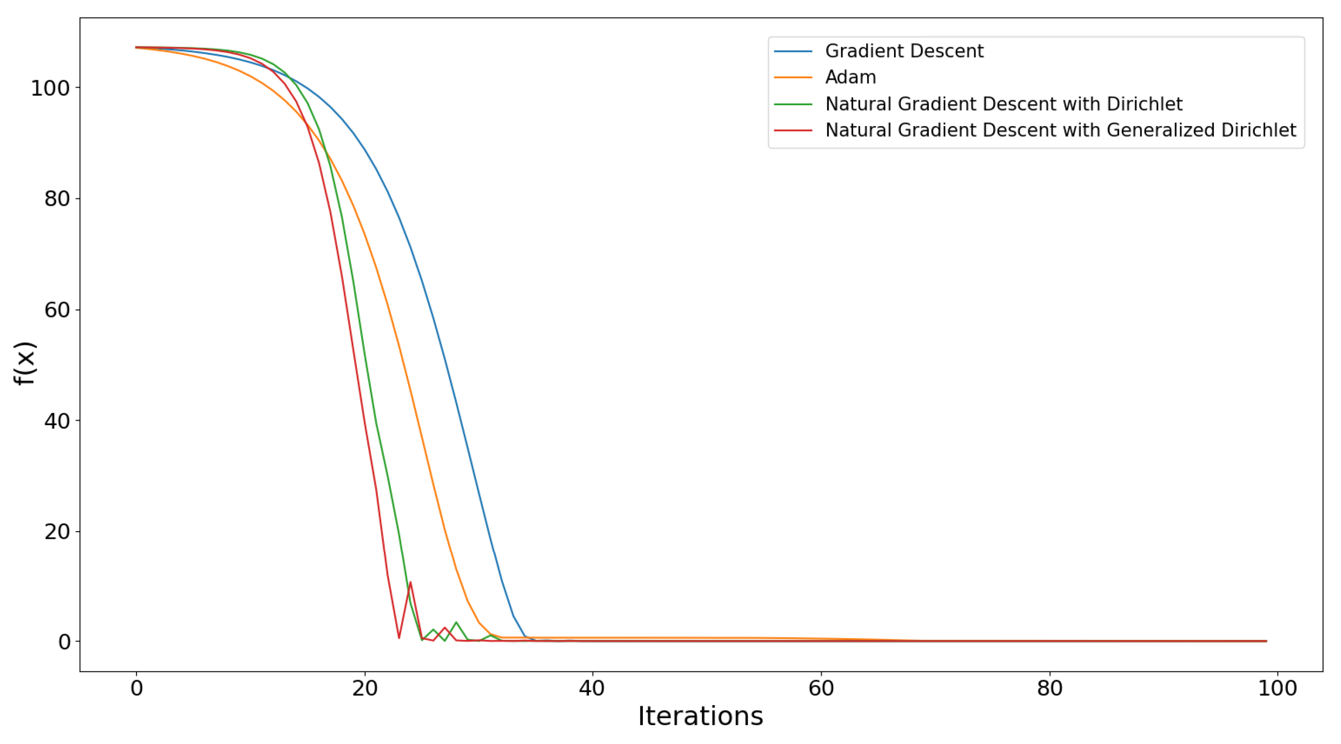
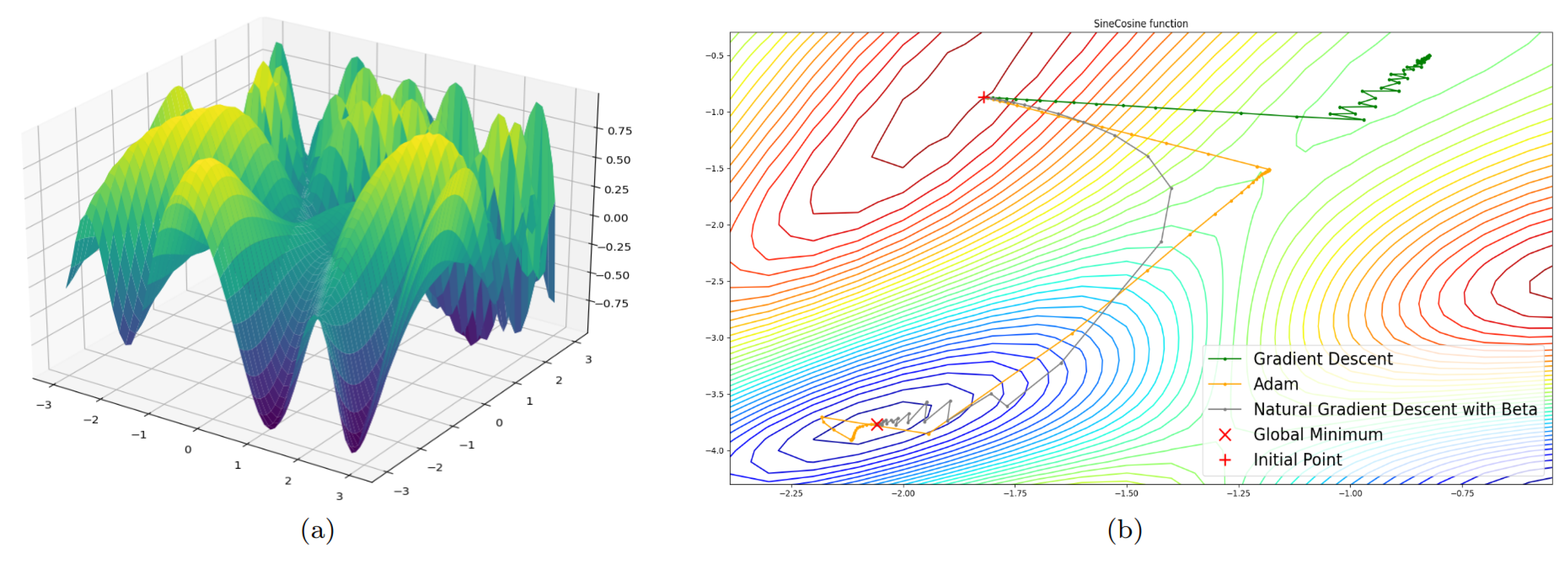
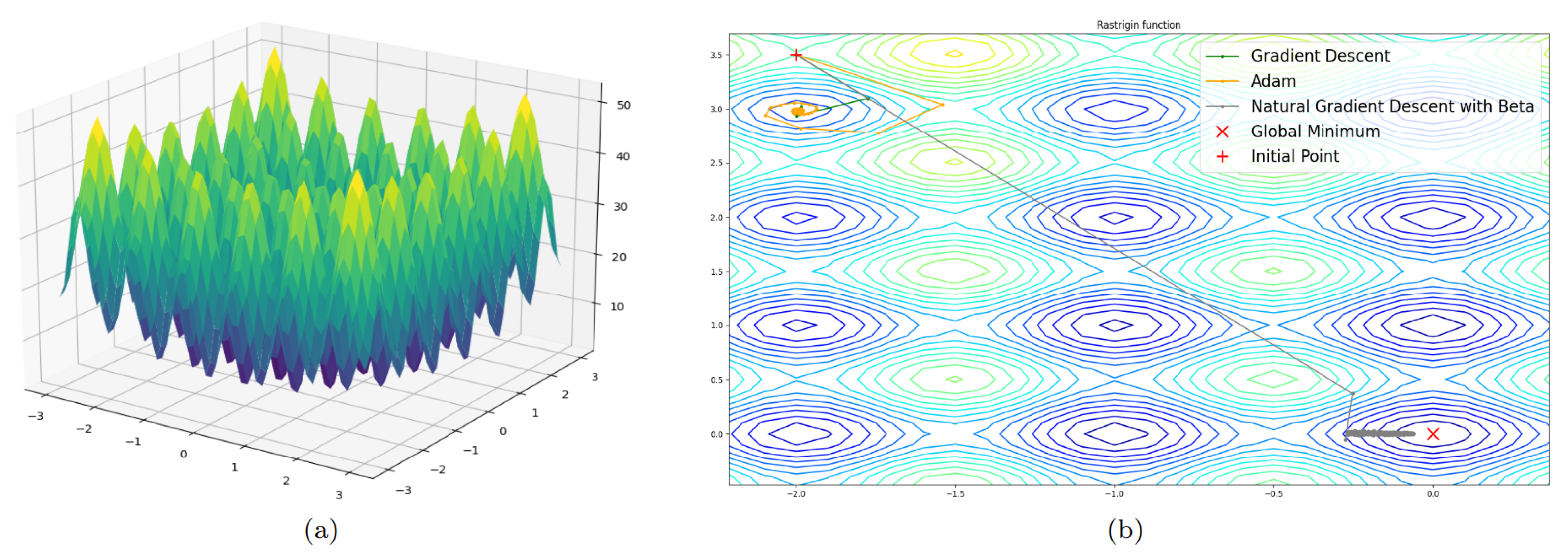
4. Experimental Part

4.1. Four-Dimensional Case

The behavior of the algorithms gradient descent with step-size adaptation and natural gradient descent of Dirichlet and general Dirichlet distributions, realized by Python 3.8.10, will be observed in experiments. We choose convex and smooth functions for solving the optimization problem.

Initial points and parameters will be defined for every function. This is intended to determine the proper distribution for every experimental function.

In the first experiment, we minimize the Rayden function, which is defined as

$$f(x)=\sum _{i=1}^4(exp(x_i)-x_i),$$

(10)

with global minimum at $x=(0,0,0,0)$, where $f(x)=4$.

Figure 1 presents that NGD with generalized Dirichlet distributions has the fastest convergence and achieves a minimal value, which is equal to $4+6e-9$. For Dirichlet distribution, the optimization is fast enough and gives the least value $4+1e-9$. For the Adam algorithm, the minimum value is $4+2e-9$. GD with step-size adaptation gives $4+2e-8$.

The second minimization is implemented on the generalized Rosenbrock function, which has the form

$$f(x)=\sum _{i=1}^3\left[100{(x_{i+1}-x_i^2)}^2+{(1-x_i)}^2\right],$$

(11)

where global minimum is equal to 0 at $x=(1,1,1,1)$.

Figure 2 shows that NGD with Dirichlet and generalized Dirichlet distributions has the fastest convergence and achieves a minimal value, which is equal to $0.01095$ and $0.22170$, respectively. For the Adam algorithm, the minimum value is $0.01391$. GD with step-size adaptation reaches $0.14325$. We can see that the proposed Algorithm 3 converges to the global minimum much earlier and gives the required accuracy compared to well-known analogs.

The extended trigonometric function is

$$f(x)=\sum _{i=1}^4{\left[\left(4-\sum _{j=1}^{4}cos{x}_i\right)+icos{x}_i-sin{x}_i\right]}^2,$$

(12)

which has the global minimum at $x=(\pi /2,\pi /2,\pi /2,\pi /2)$, where $f(x)=0$

Figure 3 demonstrates that NGD with Dirichlet distributions reaches the minimum at $1.57389e-10$. For Adam, the minimal value is $2.24709e-9$. GD with step-size adaptation shows $5.70724e-9$. NGD with Generalized Dirichlet distribution descended to $1.50210e-9$. Algorithm 3 rapidly achieves the global minimum, but, for the full convergence, takes 6–9 iterations. However, compared with Algorithms 1 and 2, our approach gives us the highest accuracy.

As we can see, the Fisher information matrix accelerates the convergence, which allows the optimizer in neural networks to work faster.

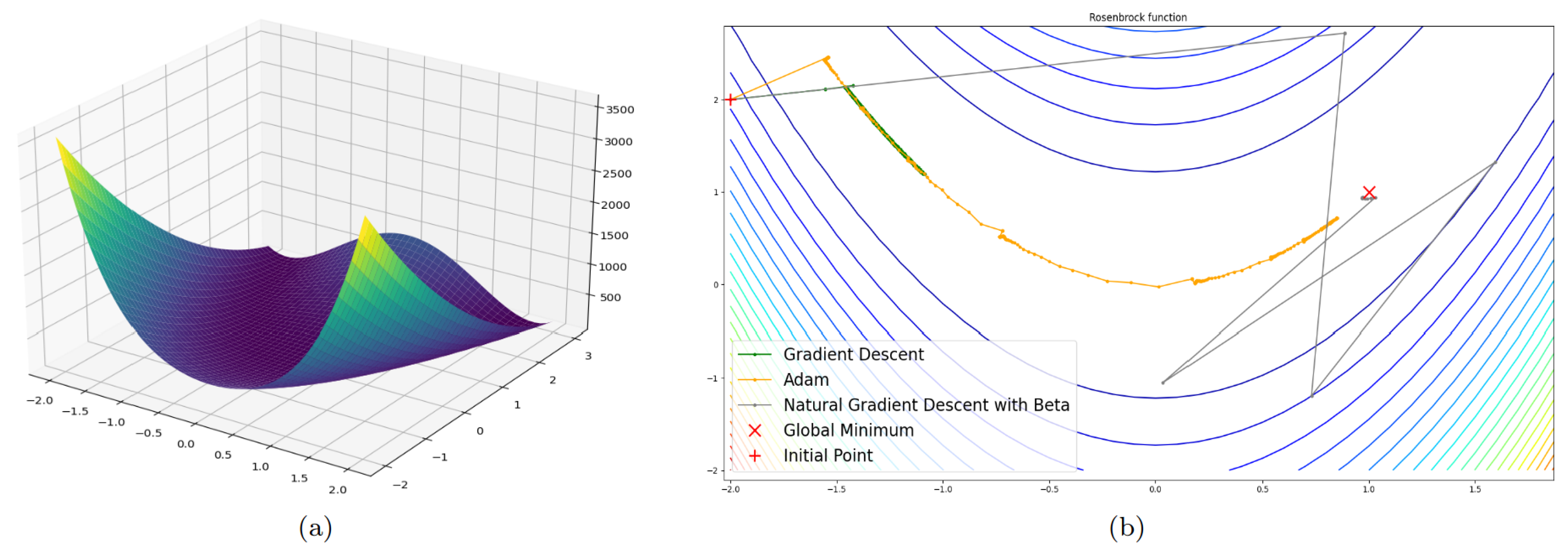
4.2. Three-Dimensional Case

In three-dimensional space, we can provide the graph of convergence and descent trajectory for each optimization method. The gradient descent and Adam algorithms with step-size adaptation remain unchanged, except the dimension of variable x. However, the Dirichlet and generalized Dirichlet distributions reduce to beta distribution.

$$p(x;a,b)=\frac{1}{B(a,b)}{x}^{a-1}{(1-x)}^{b-1},$$

(13)

where

$$\begin{array}{c}\hfill B(a,b)={\int }_0^1{t}^{a-1}{(1-t)}^{b-1}dt=\frac{\mathsf{\Gamma }(a)\mathsf{\Gamma }(b)}{\mathsf{\Gamma }(a+b)},\end{array}$$

for $0<x<1$ and $a>0,b>0$.

The beta distribution is the Dirichlet and generalized Dirichlet distribution in three-dimensional Euclidean space. Hence, the Fisher matrix of beta distribution [15] is

$$\begin{array}{c}\hfill F_{Beta}(a,b)=\left(\begin{array}{cc}{\psi }^{\prime }(a)-{\psi }^{\prime }(a+b)& -{\psi }^{\prime }(a+b)\\ -{\psi }^{\prime }(a+b)& {\psi }^{\prime }(b)-{\psi }^{\prime }(a+b)\end{array}\right).\end{array}$$

(14)

In the case of two-dimensional surfaces, we can observe their graphs and descent trajectories for each optimization method. This allows us to understand the work of every algorithm and estimate the efficiency of their models.

The surface, which is described as

$$f(x,y)=sin(\frac{1}{2}{x}^2-\frac{1}{4}{y}^2+3)cos(2x+1-e^y)$$

(15)

is a Sine–Cosine function with initial point $(x,y)=(5,5)$.

The best result gives a beta distribution and achieves $-1+2e-8$. Adam shows $-1+6e-8$, but it converges slower. The gradient descent moves in the wrong direction and achieves $-0.04198$.

The second simulation was implemented on the Rastrigin function

$$f(x)=An+\sum _{i=1}^n[x_i-Acos(2\pi x_i)],$$

(16)

where $A=10$ and $x_i\in [-5.12,5.12]$. It has the global minimum at $x=(0,0)$, where $f(x)=0$.

This function contains many local minima, and a method such as gradient descent will not achieve the global minimum with a small step size. For Adam, the step size needs to be greater than $1.6$. However, for natural gradient descent with beta distribution, the step size can be less than $0.5$.

The NGD with beta distribution reached the global minimum and gave $0.69984$. Adam and GD achieved the local minima with values $12.93451$ and $12.93446$, respectively, which do not suffice for minimization. Taking into account the convexity of the minimizing function, Algorithm 3 could descend to the global minimum, unlike its analogs.

The third simulation was implemented on the Rosenbrock function

$$f(x)=\sum _{i=1}^{n-1}[100{(x_{i+1}-x_i^2)}^2+{(1-x_i)}^2].$$

(17)

This function has a global minimum at $x=(1,1)$, where $f(x)=0$.

In this case, we apply descent in the area of local minima, where, for each method, the global minimum is achieved.

The NGD with beta distribution for the least number of iterations achieved the minimum $0.00082$. The GD moves along the area of local minima, but because of the insufficient number of iterations, stops with value $4.36387$. Adam shows a similar result to GD and reaches the value $0.02243$, which is not progressive compared with NGD. As a result, we can see that the proposed algorithm gave the most minimal value, taking a significantly smaller number of iterations.

Let us summarize the results in the

Table 1. Minimum values achieved by various algorithms.

Function	Optimization Algorithms
	GD [6]	Adam [5]	Proposed
Sine–Cosine	−0.04198	$-1+6e-8$	$-1+2e-8$
Rastrigin	12.93446	12.93451	0.69984
Rosenbrock	4.36387	0.02243	0.00082

and

Table 2. Number of iterations by various algorithms.

Function	Optimization Algorithms
	GD [6]	Adam [5]	Proposed
Sine–Cosine	19	100	26
Rastrigin	5	12	32
Rosenbrock	>500	200	20

below.

According to the results of the graphs in Figure 4b, Figure 5b and Figure 6b, we can include the number of iterations in the table. We can conclude that natural gradient descent with Dirichlet (beta) distribution works better than known analogs. It is simple to implement for the program realization and, for the least number of iterations, can give the best results in the optimization process.

5. Discussion

According to the results of experiments, we can conclude that the proposed natural gradient descent with Dirichlet distributions is able to descend into the neighborhood of the global minimum. Unlike the gradient descent [6] and Adam [5], our approach takes into account not only the gradient direction, but the convexity of the minimizing function, which allows it to miss local extremes. Moreover, the accuracy is more qualified, compared with known optimization methods.

In [14], which is a continuation of [15], we explored the natural gradient descent based on Dirichlet distribution. In this research, we added and calculated the Fisher information matrix of the generalized Dirichlet distribution. Moreover, we presented the trajectories of descent of the proposed algorithm in projected 2-d space, where Dirichlet distributions transformed into beta distribution. We verified the capability of the proposed algorithm to converge in the neighborhood of the global minimum in the case of the Rastrigin and Rosenbrock functions, where known algorithms do not achieve the global minimum. Such experiments differ from the experiments in [14,15].

The developed method allows us to minimize the loss functions of various types, which increases the accuracy of neural networks. Such an approach finds its application in convolutional and recurrent neural networks. Moreover, applying the natural gradient descent in spiking and quantum neural networks can extend the class of problems from recognition and prediction to temporal dynamics [19] and quantum computing [20]. There is a possibility to apply natural gradient descent with Dirichlet distributions in physics-informed neural networks [21], where the accuracy of solutions fully depends on the quality of minimization of the loss function.

In further research, we can examine the behavior of the natural gradient descent algorithm with the Fisher matrix of other distributions, such as gamma [22], Gompertz [23], or Gumbel [24] distributions. Moreover, we can reduce the Riemannian gradient flow to another smooth manifold besides the manifold of the probability distribution, which can potentially facilitate the optimization of the method.

References

1. Ward, R.; Wu, X.; Bottou, L. AdaGrad Stepsizes: Sharp Convergence Over Nonconvex Landscapes. J. Mach. Learn. Res. 2020, 21, 1–30. [Google Scholar]
2. Duchi, J.; Hazan, E.; Singer, Y. Adaptive subgradient methods for online learning and stochastic optimization. J. Mach. Learn. Res. 2011, 12, 2121–2159. [Google Scholar]
3. Xu, D.; Zhang, S.; Zhang, H.; Mandic, D.P. Convergence of the RMSProp deep learning method with penalty for nonconvex optimization. Neural Netw. 2021, 139, 17–23. [Google Scholar] [CrossRef] [PubMed]
4. Qu, Z.; Yuan, S.; Chi, R.; Chang, L.; Zhao, L. Genetic Optimization Method of Pantograph and Catenary Comprehensive Monitor Status Prediction Model Based on Adadelta Deep Neural Network. IEEE Access 2019, 7, 23210–23221. [Google Scholar] [CrossRef]
5. Wu, H.-P.; Li, L. The BP Neural Network with Adam Optimizer for Predicting Audit Opinions of Listed Companies. IAENG Int. J. Comput. Sci. 2021, 48, 364–368. [Google Scholar]
6. Toussaint, M. Lecture Notes: Some Notes on Sradient Descent; Machine Learning & Robotics Lab, FU Berlin: Berlin, Germany, 2012. [Google Scholar]
7. Wang, S.; Teng, Y.; Perdikaris, P. Understanding and Mitigating Gradient Flow Pathologies in Physics-Informed Neural Networks. SIAM J. Sci. Comput. 2021, 43, 3055–3081. [Google Scholar] [CrossRef]
8. Martens, J. New Insights and Perspectives on the Natural Gradient Method. J. Mach. Learn. Res. 2020, 21, 1–76. [Google Scholar]
9. Huang, Y.; Zhang, Y.; Chambers, J.A. A Novel Kullback–Leibler Divergence Minimization-Based Adaptive Student’s t-Filter. IEEE Trans. Signal Process. 2019, 67, 5417–5432. [Google Scholar] [CrossRef]
10. Asperti, A.; Trentin, M. Balancing Reconstruction Error and Kullback-Leibler Divergence in Variational Autoencoders. IEEE Access 2019, 8, 199440–199448. [Google Scholar] [CrossRef]
11. Heck, D.W.; Moshagen, M.; Erdfelder, E. Model selection by minimum description length: Lower-bound sample sizes for the Fisher information approximation. J. Math. Psychol. 2014, 60, 29–34. [Google Scholar] [CrossRef]
12. Spall, J.C. Monte Carlo Computation of the Fisher Information Matrix in Nonstandard Settings. J. Comput. Graph. Stat. 2012, 14, 889–909. [Google Scholar] [CrossRef]
13. Alvarez, F.; Bolte, J.; Brahic, O. Hessian Riemannian Gradient Flows in Convex Programming. Soc. Ind. Appl. Math. 2004, 43, 68–73. [Google Scholar] [CrossRef]
14. Abdulkadirov, R.; Lyakhov, P. Improving Extreme Search with Natural Gradient Descent Using Dirichlet Distribution. In Mathematics and Its Applications in New Computer Systems; MANCS 2021; Lecture Notes in Networks and Systems; Springer: Cham, Switzerland, 2022; Volume 424, pp. 19–28. [Google Scholar]
15. Lyakhov, P.; Abdulkadirov, R. Accelerating Extreme Search Based on Natural Gradient Descent with Beta Distribution. In Proceedings of the 2021 International Conference Engineering and Telecommunication (En&T), Online, 24–25 November 2021; pp. 1–5. [Google Scholar]
16. Celledoni, E.; Eidnes, S.; Owren, B.; Ringholm, T. Dissipative Numerical Schemes on Riemannian Manifolds with Applications to Gradient Flows. SIAM J. Sci. Comput. 2018, 40, A3789–A3806. [Google Scholar] [CrossRef]
17. Liao, Z.; Drummond, T.; Reid, I.; Carneiro, G. Approximate Fisher Information Matrix to Characterize the Training of Deep Neural Networks. IEEE Trans. Pattern Anal. Mach. Intell. 2020, 42, 15–26. [Google Scholar] [CrossRef] [PubMed] [Green Version]
18. Wong, T.-T. Generalized Dirichlet distribution in Bayesian analysis. Appl. Math. Comput. 1998, 97, 165–181. [Google Scholar] [CrossRef]
19. Wang, X.; Lin, X.; Dang, X. Supervised learning in spiking neural networks: A review of algorithms and evaluations. Neural Netw. 2020, 125, 258–280. [Google Scholar] [CrossRef] [PubMed]
20. Abbas, A.; Sutter, D.; Zoufal, C.; Figalli, A. The power of quantum neural networks. Nat. Comput. Sci. 2021, 1, 403–409. [Google Scholar] [CrossRef]
21. Guo, Y.; Cao, X.; Liu, B.; Gao, M. Solving Partial Differential Equations Using Deep Learning and Physical Constraints. Appl. Sci. 2020, 10, 5917. [Google Scholar] [CrossRef]
22. Klakattawi, H.S. The Weibull-Gamma Distribution: Properties and Applications. Entropy 2019, 21, 438. [Google Scholar] [CrossRef] [PubMed]
23. Bantan, R.A.R.; Jamal, F.; Chesneau, C.; Elgarhy, M. Theory and Applications of the Unit Gamma/Gompertz Distribution. Mathematics 2021, 9, 1850. [Google Scholar]
24. Gómez, M.Y.; Bolfarine, H.; Gómez, H.W. Gumbel distribution with heavy tails and applications to environmental data. Math. Comput. Simul. 2019, 157, 115–129. [Google Scholar] [CrossRef]
Figure 1. The rate of convergence on Rayden function using various algorithms.
Mathematics 10 03556 g001
Figure 2. The rate of convergence on generalized Rosenbrock function using various algorithms.
Mathematics 10 03556 g002
Figure 3. The rate of convergence on extended trigonometric function using various algorithms.
Mathematics 10 03556 g003
Figure 4. Experiment on Sine–Cosine function: (a) the appearance of the function; (b) the trajectory of movement to a minimum using various algorithms.
Mathematics 10 03556 g004
Figure 5. Experiment on Rastrigin function: (a) the appearance of the function; (b) the trajectory of movement to a minimum using various algorithms.
Mathematics 10 03556 g005
Figure 6. Experiment on Rosenbrock function: (a) the appearance of the function; (b) the trajectory of movement to a minimum using various algorithms.
Mathematics 10 03556 g006