Accuracy of Variational Formulation to Model the Thermomechanical Problem and to Predict Failure in Metallic Materials

Abstract

The main purpose of this study is to develop a variational formulation for predicting structure behavior and accounting for damage mechanics in metallic materials. Mechanical and coupled thermomechanical models are used to predict failure in manufacturing processes. Ductile failure is accompanied by a significant amount of plastic deformation in metallic structural components. Finite element simulation of damage evolution in ductile solids is presented in this paper. Uncoupled models are implemented in a finite element model simulating deep drawing as well as cutting processes. Based on the Johnson–Cook model, the effect of deformation on the evolution of flow stress is described. The combined effect of strain, strain rate, and temperature on plasticity and damage behavior in cutting processes is considered. The accuracy of these models is verified when predicting ductile damage in forming and cutting processes.

1. Introduction

Using both plasticity and damage mechanics is a difficult task in engineering applications. The aim of the mechanical engineer is to limit crack propagation in order to prevent the deterioration of the functionality of the structure. The finite element method is increasingly employed to predict crack propagation and optimize manufacturing processes in some applications. It has been developed from two-dimensional to multiphysics three-dimensional analysis, including failure and microstructural analysis. A coupled thermomechanical modeling is usually needed to analyze manufacturing processes. The brick elements with coupled displacement and temperature fields should be used in the modeling of these processes.

Several numerical models based on the finite element method have been developed to simulate ductile failure in metal forming. This is useful to avoid obtaining a damaged workpiece in forging, stamping, and drawing operations and developing the damage initiation and propagation in machining processes. Damage mechanics assume that the decrease in material strength is due to the nucleation of micro-cracks, their growth, and their coalescence into failure [1,2]. In continuum damage mechanics, failure is considered one of the internal state variables. The damage parameter relates to the material behavior induced by the irreversible failure of its microstructure. The effective stress depends on the damage variable. In the first, the effective scalar stress was defined [3] in order to characterize ductile damage. In addition, a variety of models was developed, and their accuracy was studied. Classification of failure models distinguishes between coupled models, where the damage evolution and the strength of the material properties are interdependent, and decoupled models. In the last one, the damage variable and plasticity fields are independent. Some research works [4,5,6] summarized and compared various ductile damage models. Indeed, many studies considered coupled damage models, such as the Lemaitre model [7,8,9,10], the Gurson model [11], and the Rousselier model [12]. These models give a more realistic prediction of damage since they take into account the interaction between mechanical behavior and damage evolution. However, the identification of the high number of related parameters is complicated. It could reduce the accuracy of the obtained models.

Nevertheless, the decoupled models are easier to implement numerically in comparison to coupled ones. As a decoupled model, the Johnson–Cook laws [13,14] predict the plastic responses, which are considered strain hardening, strain rate sensitivity, and thermal softening. They calculate fracture strains as a function of the triaxiality variable, strain rate, and temperature fields. The triaxiality is calculated as the ratio of the first stress invariant and the second one. The Johnson–Cook hardening model is the most well-known viscoplastic strain flow. Their plasticity model considers both kinematic strengthening and adiabatic heating. It describes the dynamic behavior of materials that works in diverse thermal conditions. For these advantages, these decoupled models are usually used in the simulation of metal-cutting forming processes. They involve high strains, strain rates, and temperatures, which is proven in recent works such as the work of Xuehong et al. [15], Joshua et al., [16] and Timothy et al., [17]. The accuracy of the Johnson–Cook models is checked when predicting ductile damage in bulk metal processes [18,19,20].

The accuracy of any numerical simulation is usually dependent on the accuracy of material behavior and failure modeling. In addition, the setting of behavior and damage characterization tests is crucial for an accurate material modelling. A combined experimental and numerical analysis should be developed in order to calibrate the material models. Plasticity characterization can be carried out with traction or compression tests. The ductile rupture function expresses the relation between strain at fracture and triaxiality. Characterization tests of ductile rupture should involve a wide range of stress states, such as compression and tension. The most known stress state indicator is triaxiality. In order to have various stress states in these characterization tests, different geometries of specimens are used, and tests are applied for different loading speeds. The classical failure characterization is tensile tests on smooth and notched specimens [21,22]. An optimization procedure is described [23] in order to determine the Johnson–Cook material model parameters, especially the parameter of strain rate effect. This work combines the design of experiment technique, finite element method, and an evolutionary algorithm. A ball impact test is modeled to study the behavior of metal sheets during this impact.

Today, complex manufacturing processes are often addressed with multiphysics models involving computational solid. The development in numerical modeling of material behavior has increased the ability of complex software to be used for the optimization of manufacturing processes. For example, a coupled thermomechanical three-dimensional model for FSW using the Johnson–Cook model combined with the arbitrary Lagrangian–Eulerian formulation has been developed [24]. In another study [25], the effect of hardening laws and thermal softening on predicting residual stresses in FSW of aluminum alloys has been studied. In this study, the thermal-mechanical model is coupled with stress analysis, including a metallurgical model.

This paper is divided into two parts. In the first part, the discretization of the variational formulation of the mechanical model is detailed. This model is identified to simulate the deep-drawing process, which is the manufacturing technique used for sheet metal processing, where the part is subjected to compressive loading. The material is produced at a temperature below the recrystallization temperature. Deep-drawing experiments are illustrated to prove the effectiveness of Johnson–Cook models, which depend only on the strain. In the second part, the discretization of the variational formulation of the thermomechanical model is presented. The numerical implementation of this model is used to simulate the ductile behavior and fracture in the cutting process of nonalloy steel material. The governing equations of the thermal and mechanical systems have to be studied separately using the virtual work principle. The innovation of this study is the development of thermomechanical modeling of the cutting operation using the finite element method. The Johnson–Cook model is described to illustrate the combined effect of strain, strain rate, and temperature fields on the evolution of flow stress as revealed by experiments in cutting processes.

2. Numerical Formulation of Mechanical Problem

2.1. Governing Equations of Mechanical Problem

In this section, the mechanical governing equations of a solid are presented in order to set up a finite element simulation. This aim is accomplished by specifying the equilibrium of forces equation, the compatibility equation, the constitutive behavior law, and the boundary and initial conditions for this problem. Additionally, failure mechanics and properties of the contact model should be added. The governing motion equation in a dynamic system is given in Equation (1).

$$\nabla \sigma +f_v=\rho \ddot{U}$$

(1)

where $\nabla$ is the gradient operator, σ is the stress tensor, f_v is the body force density and $\ddot{U}$ is the acceleration. The compatibility equation is the relation between strains and displacements (Equation (2)).

$$\epsilon =\frac{\nabla U+{\left(\nabla U\right)}^{tr}}{2}$$

(2)

The formulation of the elastoplastic mechanical problem requires the decomposition of the deformation tensor (Equation (3)) into elastic and plastic parts.

$$\epsilon ={\epsilon }_{el}+{\epsilon }_{pl}$$

(3)

The Johnson–Cook modified models are used with consideration that the strain rate and the temperature effects are not investigated. Therefore, we have plasticity law as Equation (4).

$${\sigma }_{eq}=\left(A+B{\epsilon }_{pl}^n\right)$$

(4)

where A, B, and n are material constants that are determined experimentally. ɛ_pl is the equivalent plastic strain. In this model, strain rate strengthening and thermal softening have neglected effects on the equivalent plastic stress. Fracture modeling is based on the calculation of the cumulative damage parameter D (Equation (5)).

$$D={\displaystyle \sum \left(\frac{\Delta {\epsilon }_{pl}}{{\epsilon }_f}\right)}$$

(5)

The damage parameter D gives the formulation of the behavior curve. D = 0 from the point of the unbroken ductile piece. Whereas when damage occurs, D = 1. By neglecting the effects of strain rate and temperature, the Johnson–Cook failure model law (Equation (6)) describes the fracture strain (${\epsilon }_f$) as a function only of stress triaxiality (η).

$${\epsilon }_f=\left(D_1+D_2 e^{D_3\eta }\right)$$

(6)

The triaxiality (Equation (7)) describes the influence of the stress state on the failure strain. The material parameters should be identified using characterization tests. The triaxiality calculated is a dimensionless ratio of hydrostatic stress (Equation (8)) to von Mises’s equivalent one (Equation (9)):

$$\eta =\frac{{\sigma }_m}{{\sigma }_{eq}}$$

(7)

The hydrostatic stress σ_m is calculated as follows:

$${\sigma }_m=\frac{{\sigma }_1+{\sigma }_2+{\sigma }_3}{3}$$

(8)

The Von Mises equivalent stress σ_eq is calculated as follows:

$${\sigma }_{eq}=\sqrt{\frac{1}{2}\left[{\left({\sigma }_1-{\sigma }_2\right)}^2+{\left({\sigma }_2-{\sigma }_3\right)}^2+{\left({\sigma }_3-{\sigma }_1\right)}^2\right]}$$

(9)

σ₁, σ₂, and σ₃ are principal tensor stresses with the assumption that σ₁ ≥ σ₂ ≥ σ₃.

In forming and cutting simulation, friction occurs at the interface between tools and workpieces.

In fact, the accuracy of computed results in finite element modeling, cutting, and forming processes is greatly dependent on the friction model along the interface workpiece/tools. Using different friction models and different friction factors affects numerical results, especially in terms of stress states. In reality, friction greatly influences the specimens’ final shape and, thus, the triaxiality. In this regard, we use the Coulomb–Tresca friction model as illustrated in system Equation (10). The shear friction stress τ_f is proportional to the shear flow stress k with the constant shear friction factor denoted m ∈ [0,1].

$${\tau }_f=\left\{\begin{array}{l}\mu {\sigma }_n\hspace{1em}if\hspace{1em}{\tau }_f<{\tau }_{\max }\\ mk\hspace{1em}if\hspace{1em}{\tau }_f\ge {\tau }_{\max }\end{array}\right.$$

(10)

where μ is the Coulomb friction coefficient, σ_n is the normal contact stress, and τ_max is the maximal shear stress.

In a current configuration, the measure of force per unit area acting on a surface is given by the stress boundary condition $\sigma n=T$ where σ is the Cauchy stress tensor, the stress vector is $T={\left\{t_x,t_y,t_z\right\}}^{tr}$ and n is the unit normal vector to a boundary element on the stress surface.

2.2. Discretization of the Variational Formulation of Mechanical Problem

The variational weak form is formulated based on the virtual work principle of Alembert [26]. The dynamic mechanical system is decomposed into many interconnected components. This statement permits to study of the stability and the equilibrium of a continuum solid subjected to infinitesimal virtual displacement Δδ in a way that the total virtual work from external and internal forces disappears [27]. The variational equation for the mechanical problem is formulated as follows in Equation (11).

$$-{\displaystyle \underset{V}{\int }\sigma \delta \dot{U} dV}+{\displaystyle \underset{V}{\int }{f}_v \delta U dV}+{\displaystyle \underset{S_f}{\int }{F}_f \delta U dS}+{\displaystyle \underset{S_{\sigma }}{\int }T \delta U dS}-{\displaystyle \underset{V}{\int }\rho \ddot{U} \delta U dV}=0$$

(11)

where, ${\displaystyle \underset{V}{\int }\sigma \delta \dot{U} dV}$ and ${\displaystyle \underset{V}{\int }{f}_v \delta U dV}+{\displaystyle \underset{S_f}{\int }{F}_f \delta U dS}+{\displaystyle \underset{S_{\sigma }}{\int }T \delta U dS}$ is the internal and the total external virtual works, respectively. The f_v is the density of volume force. The last term, ${\displaystyle \underset{V}{\int }\rho \ddot{U} \delta U dV}$ is the virtual work performed by inertial force. The contact force F_f (Equation (12)) can be decomposed into normal and tangential forces:

$$F_f=F_f^n+F_f^t$$

(12)

In order to simplify the calculation of equilibrium, the continuum system is discretized in time as well as in space using the FEM. Time discretization means to decompose the period [0, t] into determined time steps Δt.

The domain $V={\displaystyle \underset{n}{\cup }{V}_j}$ is decomposed into n finite elements connected at their nodes. V_j is the volume of each element. The time-dependent displacement of node k of element j is noted $u_j^k\left(x,y,z,t\right)$. The function approximation of the element displacement and the arbitrary displacement is expressed in system Equation (13).

$$\begin{array}{c}{u}_j={\displaystyle \sum _k{\phi }_k{u}_j^k}\\ \delta u_j={\displaystyle \sum _k{\phi }_k\delta u_j^k}\end{array}$$

(13)

where ϕ_k is the shape function at the node k and $\left(\xi ,\eta ,\zeta \right)$ are the isoparametric coordinates of this node k. This shape function is described [28] by Equation (14).

$${\varphi }_k\left(\xi ,\eta ,\zeta \right)=\frac{1}{8}\left(1+\xi {\xi }_k\right) \left(1+\eta {\eta }_k\right) \left(1+\zeta {\zeta }_k\right)$$

(14)

The shape matrix at the node k is given in Equation (15).

$$\left[{\phi }_k\right]=\left[\begin{array}{ccc}{\phi }_k& 0& 0\\ 0& {\phi }_k& 0\\ 0& 0& {\phi }_k\end{array}\right]$$

(15)

Based on Equation (11), the mechanical equilibrium is rewritten in Equation (16)

$$-{\displaystyle \underset{V}{\int }{\left[B\right]}^{tr}\sigma dV+{\displaystyle \underset{V}{\int }{\left[\varphi \right]}^{tr}{f}_v dV+{\displaystyle \underset{S_f}{\int }{\left[\varphi \right]}^{tr}{F}_f dS}}}+{\displaystyle \underset{S_{\sigma }}{\int }{\left[\varphi \right]}^{tr}T dS}-{\displaystyle \underset{V}{\int }\rho {\left[\varphi \right]}^{tr}\left[\varphi \right]} \ddot{U}dV=0$$

(16)

The semi-discrete equations of the mechanical problem at the node k of an element j can be expressed by the algebraic Equation (17).

$$\left( \left[M_j^{ki}\right]{ü}_j^i-\left\{F_{j/ext}^k\right\}+\left\{F_{j/\mathrm{int}}^k\right\}-\left\{F_{j/f}^k\right\}\right) \delta u_j^k=0$$

(17)

where $\left[M_j^{ki}\right]$ is the mass matrix of the element j, ${ü}_j^i$ is the acceleration at the node i of the element j, $\left\{F_{j/ext}^k\right\}$ is the external forces vector at the node k of the element j, $\left\{F_{j/\mathrm{int}}^k\right\}$ is the external forces vector at the node k of the element j and $\left\{F_{j/f}^k\right\}$ is the external forces vector at the node k of the element j:

$$\begin{array}{c}\left[M_j^{ki}\right]={\displaystyle {\int }_{V_j}\rho {\left[{\phi }_k\right]}^T\left[{\phi }_i\right]dV}\\ \left\{F_{j/ext}^k\right\}={\displaystyle \underset{V_j}{\int }{\left[{\varphi }_k\right]}^T{f}_v dV+}{\displaystyle \underset{S_j/S_{\sigma }}{\int }{\left[{\varphi }_k\right]}^{T}T dS}\\ \left\{F_{j/\mathrm{int}}^k\right\}={\displaystyle \underset{V_j}{\int }{\left[B_k\right]}^T\sigma dV}\\ \left\{F_{j/f}^k\right\}={\displaystyle \underset{S_j/S_f}{\int }{\left[{\varphi }_k\right]}^T{F}_f dS}\end{array}$$

(18)

where $\left[B_k\right]$ is the strain-displacement matrix. It relies on the shape function matrix (Equation (15)) with the differential matrix:

$$\left[B_k\right]=\left[\begin{array}{ccc}\partial /\partial x& 0& 0\\ 0& \partial /\partial y& 0\\ 0& 0& \partial /\partial z\\ \partial /\partial y& \partial /\partial x& 0\\ 0& \partial /\partial z& \partial /\partial y\\ \partial /\partial z& 0& \partial /\partial x\end{array}\right]\left[{\phi }_k\right]$$

(19)

σ is the Cauchy vector. It is expressed as follows ${\sigma }^{tr}=\left\{{\sigma }_{xx},{\sigma }_{yy},{\sigma }_{zz},{\sigma }_{xy},{\sigma }_{yz},{\sigma }_{zx}\right\}$. The semi-discrete equation of the mechanical equilibrium is the summation over all the n elements:

$$\left({\displaystyle \sum _{j=1}^n\left(\left[M_j^{ki}\right] {ü}_j^i-\left\{F_{j/ext}^k\right\}+\left\{F_{j/\mathrm{int}}^k\right\}-\left\{F_{j/f}^k\right\}\right)}\right) \delta u^k=0$$

(20)

The mechanical equilibrium Equation (20) can be rewritten in the semi-discrete form (Equation (21)) as a summation over all finite elements.

$$M\ddot{U}=\left\{F_{ext}\right\}-\left\{F_{\mathrm{int}}\right\}+\left\{F_f\right\}$$

(21)

where M is the mass matrix, {F_ext}, {F_int} and {F_f} are, respectively, external force vector, internal force vector and contact force vector.

$$\begin{array}{c}M={\displaystyle \sum _j{\displaystyle \underset{v}{\int }\rho {\left[\varphi \right]}^{tr}\left[\varphi \right]dV}}\\ \left\{F_{\mathrm{int}}\right\}={\displaystyle \sum _j{{\displaystyle \underset{V}{\int }\left[B\right]}}^{tr}\sigma dV}\\ \left\{F_{ext}\right\}={\displaystyle \sum _j\left({\displaystyle \underset{V}{\int }{\left[\varphi \right]}^{tr}{F}_v dV+}{\displaystyle \underset{S_{\sigma }}{\int }{\left[\varphi \right]}^{tr}T dS}\right)}\\ \left\{F_f\right\}={\displaystyle \sum _j{\displaystyle \underset{S_f}{\int }{\left[\varphi \right]}^{tr}{F}_f dS}}\end{array}$$

(22)

3. Modeling of Sheet Deep-Drawing Process

Failure analysis is an important area of engineering science to define the primary causes of failure because the strength of the material is reduced during deformation due to the occurrence of damage. Forming processes are common phenomena in the industry. The demand of mechanical industries gives the need for numerical studies of forming processes. The finite element approach is used in predicting variables that minimize the experimental procedures and reduce the product’s manufacturing costs.

3.1. Characteristics of Deep-Drawing Process

Sheet metal forming is of great importance in all industrial sectors, such as aerospace and automotive. It includes the process of deep drawing in which sheet metals undergo permanent deformation by cold forming. Deep drawing is a common process in the industry for making products from sheet metal. This process is widely used to manufacture various products, such as automotive parts. The schematic of conventional deep drawing is shown in Figure 1.

In this process, the part is placed on the die, and the blank holder is then inserted on top of the part, which is not deformed by the punch. The role of the blank holder is to control the sliding of the part during the forming process. After closing the blank holder, the punch moves down and deforms the part into its final shape. The punch has the shape of the finished product.

3.2. Identification of Plasticity and Damage Parameters

The current work is part of a comprehensive study on damage modeling of DC01 for use in the deep-drawing process. The material studied is low-carbon steel. It has a good level of ductility. The chemical composition of DC01 is illustrated in

Table 1. Chemical compositions of the DC01 steel (EN 10130).

C	Mn	P	S
≤0.12	≤0.6	≤0.045	≤0.045

.

This material is suitable for forming requirements such as deep drawing. It is used to obtain complicated component shapes when necessary and even allows for deep stamping. Here, a car fuel tank made of DC01 steel sheet is being investigated using the deep drawing process. The thickness of the blank sheet is 1.2 mm. The stress-strain curves (Figure 2) resulting from tensile tests on the sheet metal specimens cut by the wire-cutting process are shown in the figure below. Three directions corresponding to the rolling direction of the sheet (0, 45, and 90°) are used.

The variation of the three rolling directions of the sheet sample did not affect Young’s modulus, and a slight variation in the yield strength and tensile strength values. Therefore, the DC01 sheet with a thickness of 1.2 is considered an isotropic material.

3.3. Determination of Material Constants

Equation 4 can be written in logarithmic form as shown in Equation (23):

$$Ln\left({\sigma }_{eq}-A\right)=n.Ln\left({\epsilon }_{eq}\right)+Ln\left(B\right)$$

(23)

The relationship between ln(σ − A) and ln(ε_pl) is drawn in a linear curve. The first-order regression model is used to fit the data points, as represented in Figure 3.

The logarithmic curve obtained from the tensile test of specimens cut in the three rolling directions is used to calibrate the modified Johnson–Cook hardening model. Indeed, from the slope and intercept of the fitted curve, the material constants A, B and n are estimated, as shown in

Table 2. Estimation of DC01 constants A, B, and n.

A (MPa)	B	n
245	518	0.75

.

In other ways, stress triaxiality $\eta$ is well known as an important parameter in controlling failure process. It depends on critical failure strain. The computed stress triaxialities from the numerical computations are found to be significantly consistent with the theoretical results. In the case of uniaxial tension of a smooth specimen, the principal stresses in the center of the specimen are σ₂ = σ₃ = 0. Based on Equations (7)–(9), the triaxiality is η = 1/3. In addition, for the round bar specimens, the stress triaxiality states according to Bridgman’s analytical model [30] are used to cross check the numerical data.

$$\eta =\frac{1}{3}+\sqrt{2}.Ln\left(1+\frac{t}{4R}\right)$$

(24)

where ղ, R and t are the stress triaxiality, the radius of the notch and the flat thickness at the groove. Now, we determine the numerical stress states in the critical element of each sheet specimen. A variety of tensile tests is performed and the triaxiality is computed at failure. Calculated triaxiality is compared with analytical values determined by Equation (24). The triaxiality is analyzed for smooth and notched sheet specimens as presented in Figure 4.

Table 3. Comparison between theoretical and numerical triaxiality for DC01 material.

Specimen	S1	NS1	NS2	NS3
t (mm)	1.2	1.2	1.2	1.2
R (mm)	-	2	4	10
Numerical triaxiality	0.331	0.517	0.434	0.4
Theoretical triaxiality	0.33	0.531	0.436	0.375
Strain at failure	0.22	0.12	0.15	0.17

gives the theoretical and calculated values of triaxiality at failure in the critical elements of notched specimens.

As shown in system Equation (25), we neglect the effects of strain rate ɛ̇ and temperature T in the damage law. The failure model can be rewritten only in terms of the stress triaxiality effect, as described in Equation (6).

$$\begin{gathered} Ln\left(\frac{\stackrel{.}{\epsilon }}{{\stackrel{.}{\epsilon }}_0}\right)\approx 0 \\ {T}^{\ast }=\frac{T-T_0}{T_m-T_0}\approx 0 \end{gathered}$$

(25)

where ɛ̇₀ = 1 s⁻¹ as the reference strain rate and T₀ = 20 °C as a reference temperature. The the curve ${\epsilon }_f=f\left(\eta \right)$ is determined by substituting the stress triaxialities and corresponding fracture strain values into the relationship (Equation (6)). Therefore, from the coefficients of the fitted equation, the model parameters $D_1,D_2, \mathrm{and} D_3$ are computed. As shown in Figure 5, the failure model parameters D₁, D₂, and D₃ are determined.

The estimated parameters for the fracture model (Equation (6)) are presented in

Table 4. Failure constants of DC01.

D1	D2	D3
0.08	1.6	−7.2

. They will be used in metal-forming applications to predict ductile fracture in DC01 steel plates.

3.4. Experiment and Numerical Results of Car Fuel Tank Deep Drawing

In the deep-drawing process, the sheet metal is drawn radially into the die cavity by the mechanical action of a punch. Experimentally, the part is inserted into the die and clamped by the blank holder. The center of the part corresponds to the center of the die, as well as the center of the top plate. This configuration is crucial for applying the punch pressure to the center of the sheet. The sheet blank is deformed evenly in all directions, and we obtain the car tank. In fact, the forming process starts with the punch penetration to perform a drawing accompanied by a reduction in the wall thickness. The bottom of the drawn part is then formed. The simulations are performed using the modified Johnson–Cook material models (Equations (4) and (6)). The numerical simulations of the car fuel tank stamping are performed with the modified Johnson–Cook plasticity model, in which we do not consider strain rates and temperatures. This model allows us to predict the strain field during the deep-drawing process due to well-established methods to identify the material parameters. In addition, damage parameters are included in the failure model in order to illustrate the fracture behavior. We assume that the die, the blank holder, and the punch are rigid. The blank is modeled as a deformable shell. The sheet is meshed using four nodes quadrilateral shell elements S4R with reduced integration and hourglass control with five integration points through the thickness. This finite element model prepared in ABAQUS is shown in Figure 6.

The combined Coulomb–Tresca friction model (Equation (10)) is thus applied in the current paper, assuming the Tresca friction factor m = 0.45 and Coulomb factor μ_C = 0.1.

The proposed numerical model is able to predict the deep-drawing experimental results, for example, the shape of the car fuel tank and the thickness distribution (STH). In addition, the model is able to predict the damage initiation and evolution areas in this part. We illustrate in Figure 7 the wrinkling in the workpiece (first test).

During the deep-drawing operation, the stress in the flange region is a combination of radial tensile stress and tangential compressive stress (hoop stress). The main defects of deep-drawn parts are wrinkling and/or necking. Wrinkling usually occurs at the flange region by excessive compressive stresses leading to local buckling of the sheet. On the other hand, necking is due to excessive radial tensile stress. These two defects, i.e., wrinkling and necking, define the limits of the deep-drawing process. We illustrate in Figure 8 the distribution of damage parameter D (second test).

The die has r_d as the radius (Figure 1). In order to avoid the rupture of the blank in the rounded section of the die, the blank holding force should be well-determined. In fact, this force is reduced to the extent that the blank material is able to flow while avoiding wrinkles over the blank rounded sections. The results obtained in the simulations were in good agreement with the experimental observations. Furthermore, the proposed model is capable of correctly predicting the cracks’ nucleation and their evolution. The deep-drawing operation begins once the required, blank holding force has been raised to the extent that the blank material is able to flow without generating wrinkles. In this case, we obtain the rupture of the blank. In this study, numerical results of car fuel tank deep drawing concluded that the blank-holder force should be sufficient and optimized in order to prevent damage and wrinkling in the final workpiece.

4. Thermomechanical Model of Ductile Materials

4.1. Governing Equations of Thermomechanical Problem

In the finite element analysis of the mechanical problem, an essential step is assembling all the element stiffness matrices in order to obtain the stiffness matrix [K]. It is often difficult to determine this assembly matrix. For that, we briefly show the mathematical equations to solve such a problem in this section. Indeed, the discretization of a physical system is described with the algebraic Equation (26).

$$\left[K\right]\left\{X\right\}=\left\{F\right\}$$

(26)

In the second term of Equation (26), we define the force vector {F}, in which the nodal reaction forces in each node are associated with the imposed displacement and temperature nodes. {X} is a vector that contains, in a thermomechanical problem, displacements and temperature fields. The results of both fields in all nodes are placed in this vector. When the governing Equations (26) are linear, solving the problem is reached by calculating the unknown vector as shown in Equation (27).

$$\left\{X\right\}={\left[K\right]}^{-1}\left\{F\right\}$$

(27)

However, matrix inversing is impossible in the case of nonlinearity of the governing Equations (26). The problem can be solved by breaking the applied load in a step into smaller increments. This nonlinearity is due to material behavior, geometry, interactions between multiphysics systems, or boundary conditions. The finite element method is a solution to study multiphysics problems. Two mathematical formulations of multiphysics analysis can be used. They called the monolithic (coupled) and the staggered (decoupled) formulations [31]. In the coupled approach, only one set of differential equations is used. At each iteration, all variables are updated at the same time. This approach has the advantage of stability and accuracy [32]. In the case of the 3D thermomechanical model, each node has four degrees of freedom, which are three components of displacements and a thermal scalar. The staggered approach divides the multiphysics system into subsystems containing mechanical and thermal fields. Each time step is divided into some iterations in which each field is solved separately. The staggered analysis is nonlinear.

There are two coupling strategies, which are weak and strong coupling. First, for the weak coupling case, the variable’s flow has only one direction from one subsystem to another. Based on Equation (26), the weak-coupled system Equation (28) is written in the following matrix form:

$$\left[\begin{array}{cc}\left[K_{mech-mech}\right]& \left[0\right]\\ \left[0\right]& \left[K_{ther-ther}\right]\end{array}\right]\left\{\begin{array}{c}\left\{X_{mech}\right\}\\ \left\{X_{ther}\right\}\end{array}\right\}=\left\{\begin{array}{c}\left\{F_{mech}\right\}\\ \left\{F_{ther}\right\}\end{array}\right\}$$

(28)

where the indices mech and ther designate, respectively, the mechanical and the thermal fields.

On the other hand, each subsystem depends on the other for the strong coupling case. At the same time, mechanical characteristics depend strongly on the temperature field. The strong-coupled system Equation (29) is written as follows:

$$\left[\begin{array}{cc}\left[K_{mech-mech}\right]& \left[K_{mech-ther}\right]\\ \left[K_{ther-mech}\right]& \left[K_{ther-ther}\right]\end{array}\right]\left\{\begin{array}{c}\left\{X_{mech}\right\}\\ \left\{X_{ther}\right\}\end{array}\right\}=\left\{\begin{array}{c}\left\{F_{mech}\right\}\\ \left\{F_{ther}\right\}\end{array}\right\}$$

(29)

By taking into account the effect of temperature fields, mechanical governing systems are described by Equation (30):

$$\begin{array}{c}\nabla \sigma +f_v=\rho \ddot{U}\\ \dot{\epsilon }=\frac{\nabla \dot{U}+{\left(\nabla \dot{U}\right)}^T}{2}\\ \epsilon ={\epsilon }_{el}+{\epsilon }_{pl}+{\epsilon }_{th}\end{array}$$

(30)

Johnson–Cook models are commonly used in the simulation of machining processes involving high strains, strain rates, and temperatures [18,33,34]. Ductile material modeling may be described with constitutive material behavior and damage models. The equivalent plastic flow stress (Equation (31)) is decomposed into strain hardening, kinematic hardening, and thermal softening by raised temperature. We denote ɛ_pl as equivalent plastic strain. The strain rate and the reference strain rate (1 s⁻¹) are indicated by ɛ̇ and ɛ̇₀, respectively. In the therma term, T is the temperature, T₀ is the reference temperature, and T_m is the melting one.

$${\sigma }_{eq}=\left(A+B {\epsilon }_{pl}^n\right)\left(1+C Ln\left(\frac{\stackrel{.}{\epsilon }}{\stackrel{.}{{\epsilon }_0}}\right)\right)\left(1-{\left(\frac{T-T_0}{T_m-T_0}\right)}^m\right)$$

(31)

The material parameters A, B, n, C, and m are the yield stress, the strain hardening coefficient, the strain hardening exponent, the strain rate dependence coefficient, and the temperature dependence coefficient, respectively.

Equation (31) contains three components. The first one $\left(A+B {\epsilon }_{pl}^n\right)$ represents the strain hardening effect. The second one $\left(1+C Ln\left(\frac{\stackrel{.}{\epsilon }}{\stackrel{.}{{\epsilon }_0}}\right)\right)$ is the strain rate strengthening effect. The third one $\left(1-{\left(\frac{T-T_0}{T_m-T_0}\right)}^m\right)$ illustrates the temperature effect that may influence the flow stress, ${\sigma }_{eq}$, in some mechanical problems.

Fracture modeling is based on the calculation of the cumulative damage parameter D (Equation (5)). We denote $\Delta {\epsilon }_{pl}$ as the equivalent plastic strain increment.

The idea of Johnson–Cook fracture model (Equation (32)) is to describe the fracture equivalent plastic strain (${\epsilon }_{pl}$) as a function of stress triaxiality, strain rate, and temperature (T).

$${\epsilon }_{pl}=\left(D_1+D_2{ e}^{D_3\eta }\right)\left(1+D_4 Ln\left(\frac{\stackrel{.}{\epsilon }}{\stackrel{.}{{\epsilon }_0}}\right)\right)\left(1-D_5\frac{T-T_0}{T_m-T_0}\right)$$

(32)

The first term represents triaxiality. It describes the influence of the stress state on the failure strain. The second term considers the influence of strain rate $\dot{\epsilon }$ on the deformation, and the third term represents the influence of heating on the strain at the damage point. Plasticity constants (A, B, n, C, and m) and fractures (D₁ to D₅) are calculated from characterization tests at different temperatures and strain rates. In the cutting simulation, friction occurs at the interface between the tool and workpiece and chip. As explained previously, we use the combined model to predict the friction between the tool and the workpiece.

In addition, the governing thermal Equation (33) is as follows:

$$\rho Cp \dot{T}=-div\left(q\right)+Q$$

(33)

where C_p is the specific heat, Ṫ is temperature rate, Q is the internal heat generation rate per unit-deformed volume, $q=-k\nabla T$ is the heat flux, and k is the isotropic temperature-dependent thermal conductivity.

In cutting processes, heating flux Q, which is given by Equation (34), is generated from friction between the tool and workpiece as well as from plastic straining.

$$Q=Q_p+Q_f$$

(34)

The heat flux Q (Equation (36)) can be divided into Q_p, which is created from plastic work and Q_f, which is caused by friction work between workpiece and tool as well as from between chip and tool:

$$\begin{array}{c}Q=Q_{pl}+Q_f\\ Q_{pl}={\eta }_{pl} \sigma :{\dot{\epsilon }}_{pl}\\ Q_f={\eta }_f f_f {\tau }_f \dot{U}+h \left(T-T_{tool}\right)\end{array}$$

(35)

where η_p is the fraction of plastic work converted into heat, η_f is friction work conversion, f_f is the fraction of transferred friction heat to the workpiece, τ_f is the friction stress, T_tool is the temperature of the tool, and h is heat transfer coefficient due to thermal conduction. The heat convection and heat radiation are ignored. Equations (33) are rewritten as follows (Equation (36)).

$$\rho Cp \dot{T}-div\left(k\nabla T\right)-{\eta }_{pl} \sigma :{\dot{\epsilon }}_{pl}-\left({\eta }_f f_f {\tau }_f \dot{U}+h\left(T-T_{tool}\right)\right)=0$$

(36)

4.2. Discretized Form of Thermomechanical Problem

By assuming that the internal heat flux results only from plastic deformation and contact friction, the weak variational form of the thermodynamic equilibrium is given by Equation (37) expressed as a function of an arbitrary temperature variation δT.

$${\displaystyle \underset{V}{\int }\left(\rho C_p\dot{T}-div\left(k\nabla T\right)-{\eta }_{pl} \sigma :\dot{\epsilon }\right)\delta TdV}-{\displaystyle \underset{S_f}{\int }\left({\eta }_f{f}_f{\tau }_f \dot{U}+h\left(T-T_{tool}\right)\right)\delta TdS}=0$$

(37)

where δT is an arbitrary temperature variation. The workpiece has a volume V and a contact surface with tool S_f. The space of functions themselves as well as their derivatives are L²-integrable and belong to the H¹ space. Then, thermomechanical problem can be expressed as follows:

$$\begin{array}{c}-{\displaystyle \underset{V}{\int }\sigma \delta \dot{U} dV}+{\displaystyle \underset{V}{\int }{f}_v \delta U dV}+{\displaystyle \underset{S_f}{\int }{F}_f \delta U dS}+{\displaystyle \underset{S_{\sigma }}{\int }T \delta U dS}-{\displaystyle \underset{V}{\int }\rho \ddot{U} \delta U dV}=0\\ {\displaystyle \underset{V}{\int }\rho C_p\dot{T}\delta TdV}-{\displaystyle \underset{V}{\int }div\left(k\nabla T\right)\delta TdV}-{\displaystyle \underset{V}{\int }{\eta }_{pl}\sigma :\dot{\epsilon } \delta TdV}-{\displaystyle \underset{S_f}{\int }\left({\eta }_f{f}_f{\tau }_f \dot{U}+h\left(T-T_{tool}\right)\right)\delta TdS}=0\end{array}$$

(38)

where, ${\displaystyle \underset{V}{\int }\sigma \delta \dot{U} dV}$ and ${\displaystyle \underset{V}{\int }{f}_v \delta U dV}+{\displaystyle \underset{S_f}{\int }{F}_f \delta U dS}+{\displaystyle \underset{S_{\sigma }}{\int }T \delta U dS}$ represent the internal virtual work and the total external virtual work, respectively. ${\displaystyle \underset{V}{\int }\rho \ddot{U} \delta U dV}$ is the virtual work performed by inertial force. ${\displaystyle \underset{V}{\int }\rho C_p\dot{T}\delta TdV}$ represents the thermal virtual work. ${\displaystyle \underset{V}{\int }div\left(k\nabla T\right)\delta TdV}$ is the internal heat virtual work and the term ${\displaystyle \underset{V}{\int }{\eta }_{pl}\sigma :\dot{\epsilon } \delta TdV}$ represents the plastic virtual work converted into heat. Finally, the term ${\displaystyle \underset{S_f}{\int }\left({\eta }_f{f}_f{\tau }_f \dot{U}+h\left(T-T_{tool}\right)\right)\delta TdS}$ is the total friction virtual work between the workpiece and tool.

For each node k of an element j, the semi-discrete thermal energy balance is given in Equation (39):

$$\left(\left[C_j^{ki}\right]{\dot{T}}_j^i+\left[H_{j/\mathrm{int}}^k\right]\right)\delta T_j^k=0$$

(39)

where $\left[C_j^{ki}\right]$ is the capacitance matrix in the node k and $\left[H_{j/\mathrm{int}}^k\right]$ is the internal heat flux vector. We obtain the system Equation (40).

$$\begin{array}{c}\left[C_j^{ki}\right]={\displaystyle \underset{V_j}{\int }\rho C_p{\left[{\varphi }_k\right]}^{tr}\left[{\varphi }_i\right]dV}\\ \left[H_{j/\mathrm{int}}^k\right]={\displaystyle \underset{V_j}{\int }{\left[B_k\right]}^{tr}k T\left[B_k\right]dV}-{\displaystyle \underset{V_j}{\int }{\left[{\varphi }_k\right]}^{tr}{\eta }_{pl} \sigma \epsilon dV}-{\displaystyle \underset{S_f/S_j}{\int }{\left[{\varphi }_k\right]}^{tr}{Q}_f dS}\end{array}$$

(40)

Over all of the finite elements, the thermal semi-discrete equilibrium equation is given by system Equation (41).

$$\begin{array}{c}\left[C\right]\dot{T}+\left[H_{\mathrm{int}}\right]=0\\ \left[C\right]={\displaystyle \sum _j{\displaystyle \underset{V_j}{\int }\rho C_p{\left[\varphi \right]}^{tr}\left[\varphi \right]dV}}\\ \left[H_{\mathrm{int}}\right]={\displaystyle \sum _j{\displaystyle \underset{V_j}{\int }{\left[B\right]}^{tr}k T\left[B\right]dV}-{\displaystyle \underset{V_j}{\int }{\left[\varphi \right]}^{tr}{\eta }_p \sigma \epsilon dV}-{\displaystyle \underset{S_f/S_j}{\int }{\left[\varphi \right]}^{tr}{Q}_{f}dS}}\end{array}$$

(41)

In order to take into account the nonlinearities in our model, we presented a numerical method to analyze a coupled thermomechanical problem.

4.3. Determination of Material Constants

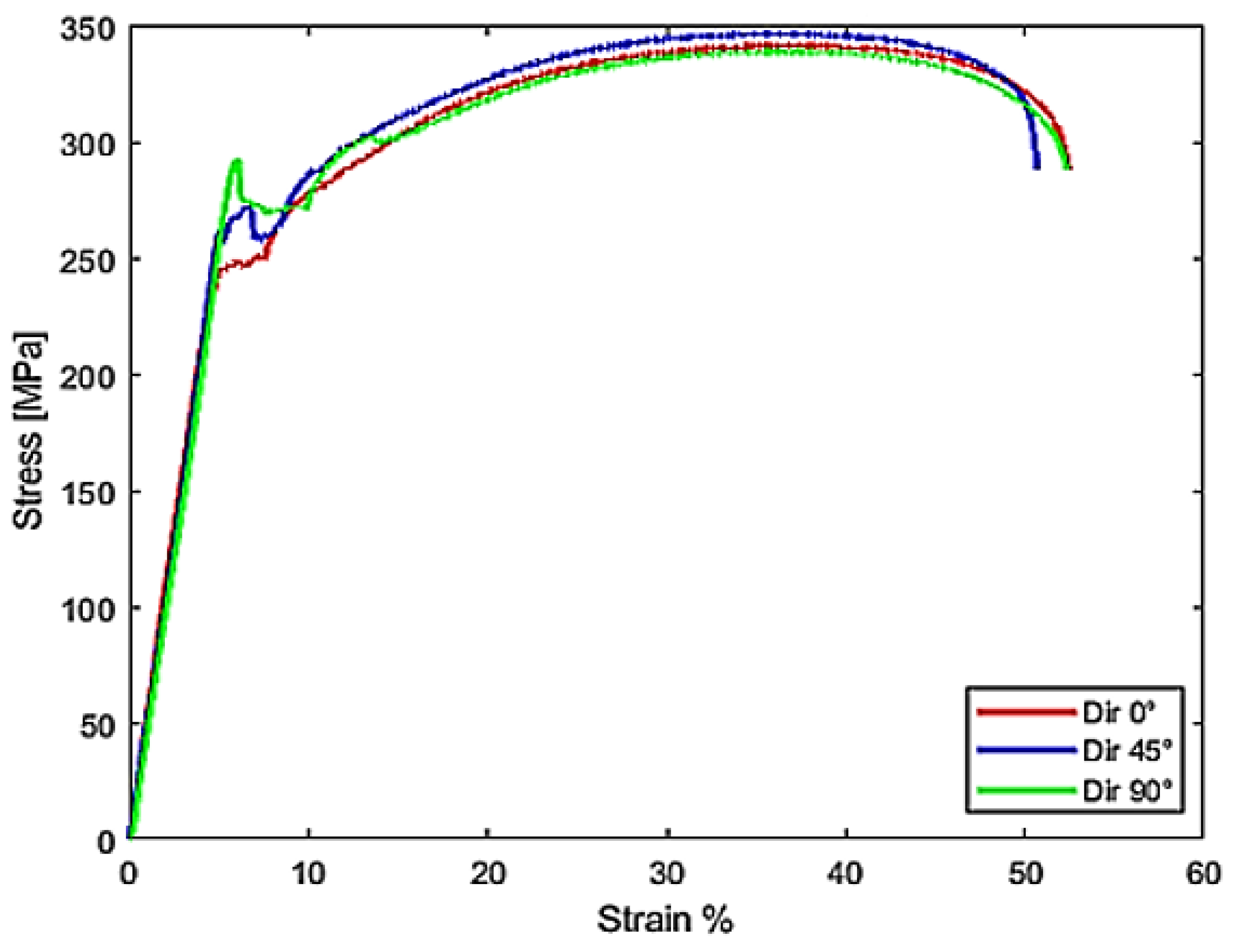
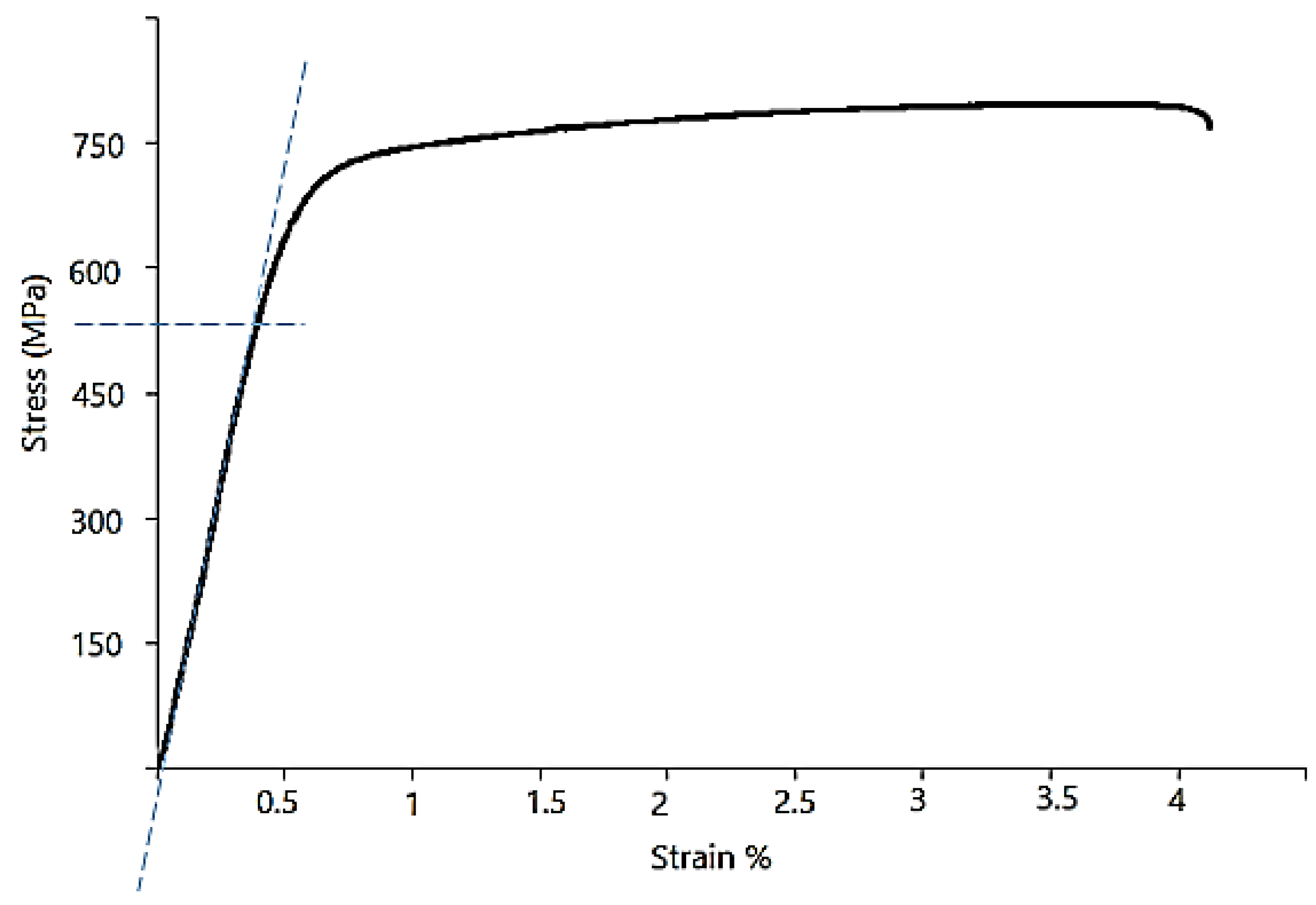
The stress-strain curve resulting from the tensile tests on the bulk specimen cut by the wire cutting process is shown in Figure 9.

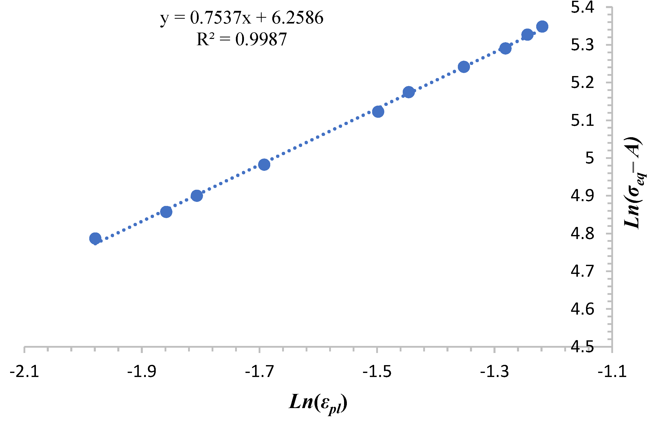
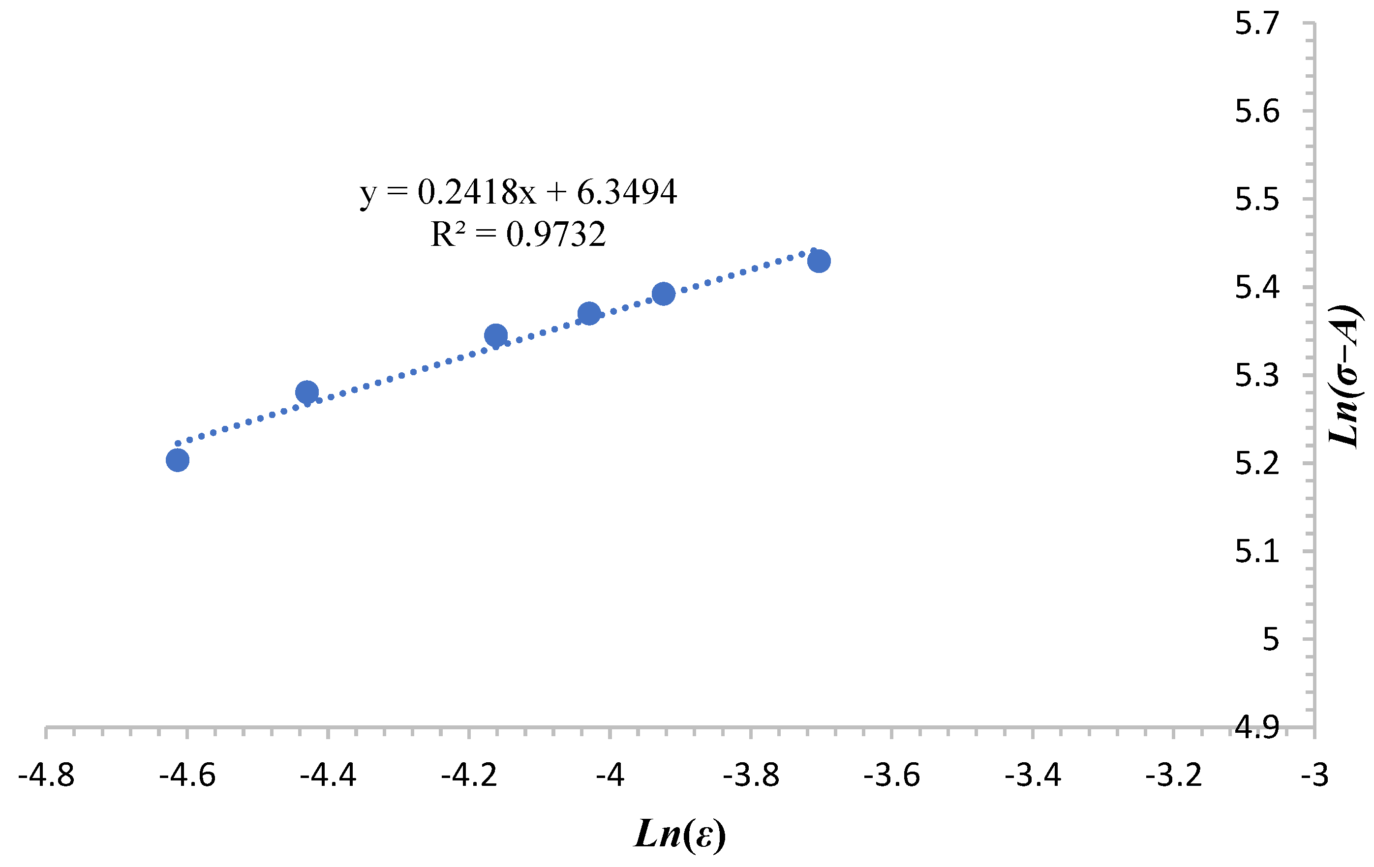
Based on the same method described previously, the linear relationship plot between ln(σ−A) and ln(ε) is represented in Figure 10.

The material constants A, B, and n are estimated as follow:

Taking a constant strain rate ${\dot{\epsilon }}_0=1 {\mathrm{s}}^{-1}$, these material constants were also determined from [35], as shown in

Table 5. Estimation of AISI1045 constants.

AISI1045 Constants	A (MPa)	B (MPa)	n	C	m
Our prediction of material constants	520	572	0.241	-	-
Material constants [35]	553	600	0.234	0.0134	1

. We chose the strengthening coefficient of strain rate, C, and the thermal softening coefficient, m, from [35]. The stress triaxiality controls the material failure through an equivalent strain at failure in cutting processes. It is estimated from the numerical simulations, and its value should be considered consistent with the analytical solutions. In addition, stress triaxiality states according to the analytical model [36] are employed to check the numerical triaxiality as illustrated in Equation (42):

$$\eta =\frac{1}{3}+Ln\left(1+\frac{a}{2R}\right)$$

(42)

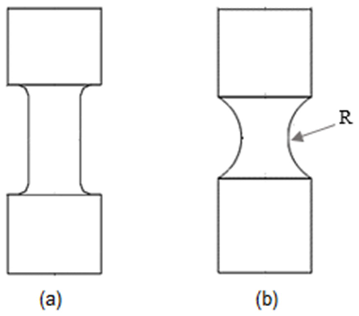
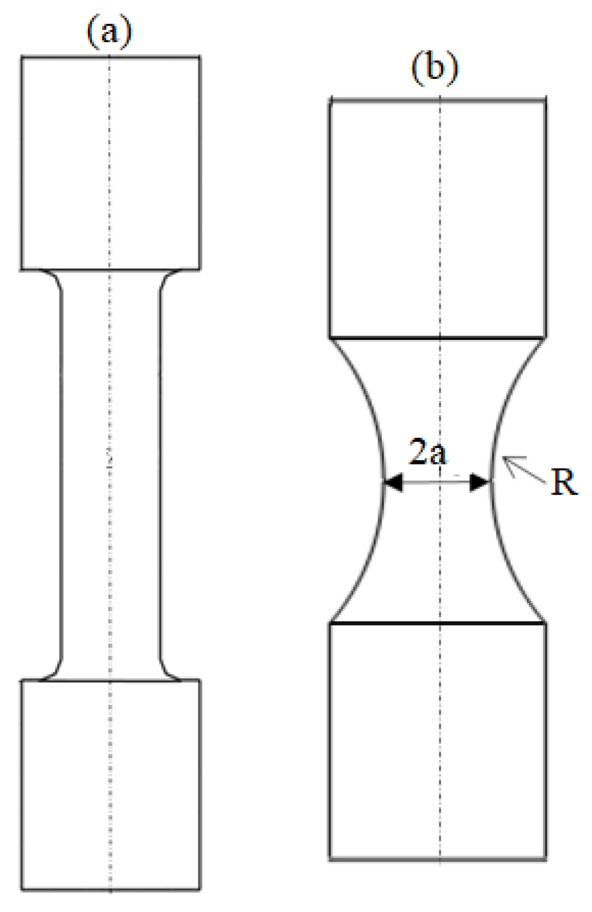
where ղ, R, and a are the stress triaxiality, the notch radius and the minimum cross- section of the radius, respectively. Computed triaxiality is compared with analytical values determined by Equation (42). The triaxiality is calculated and computed of smooth and notched specimens drawn in Figure 11.

In

Table 6. Comparison between theoretical and numerical triaxiality for AISI1045 material.

Specimen	B1	NB1	NB2	NB3
a (mm)	-	3	3.8	3.8
R (mm)	-	10	10	6.3
Numerical triaxiality	0.345	0.474	0.515	0.611
Theoretical triaxiality	0.33	0.473	0.507	0.6
Strain at failure	1.54	1.2	1.11	0.92

, we present the theoretical and computed triaxiality values at failure in the critical elements of notched specimens.

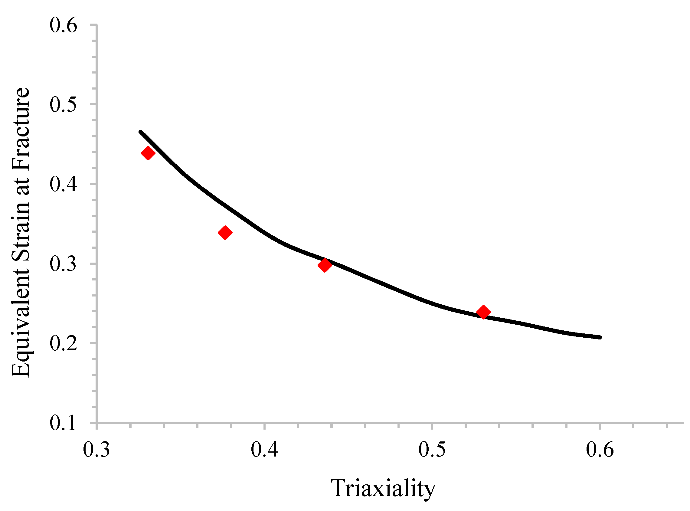
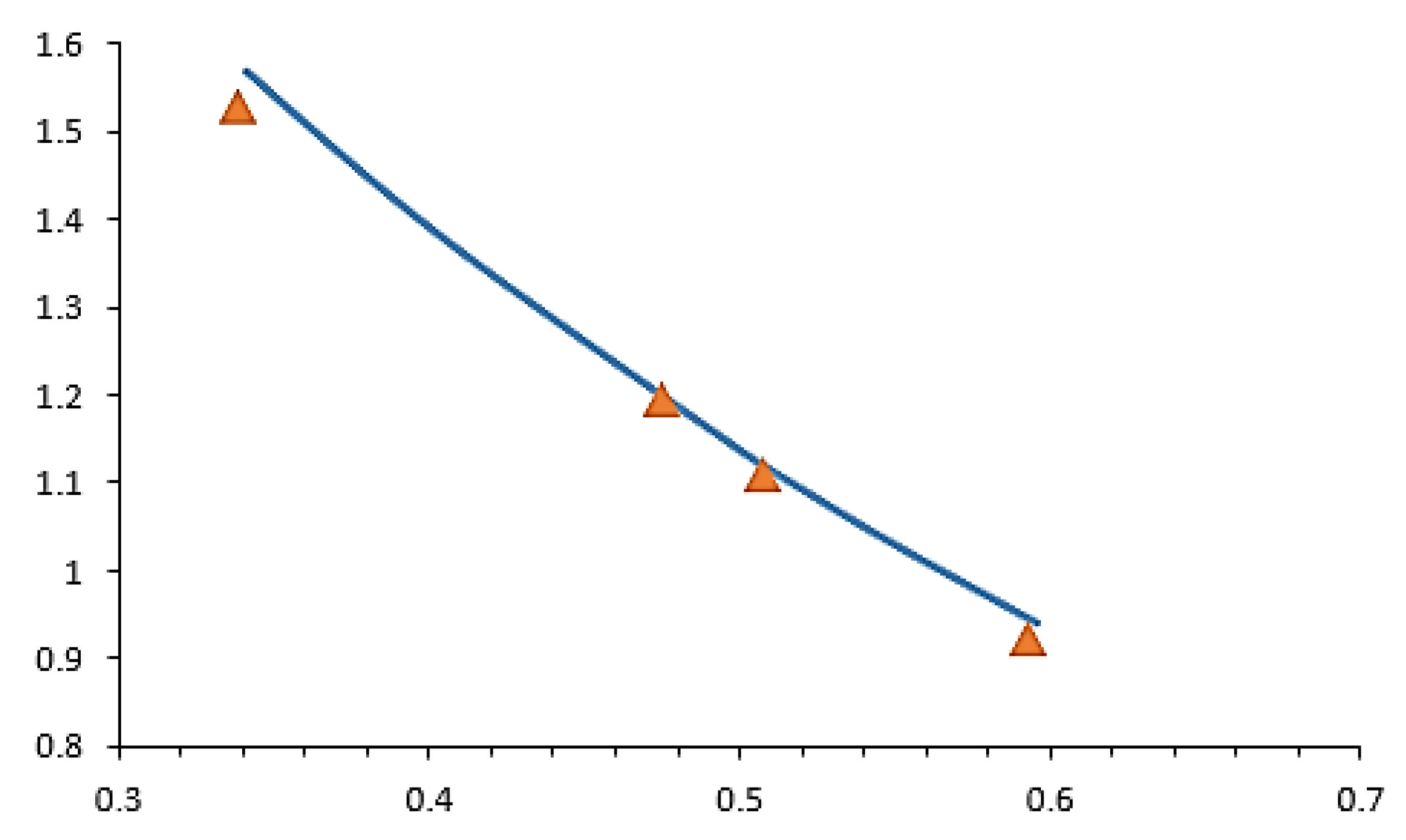
We consider the effects of strain rate and temperature on the failure model (Equation (5)). By substituting the stress triaxialities and corresponding equivalent strain at fracture into the relationship (Equation (5)), the curve ${\epsilon }_f=f\left(\eta \right)$ is determined. Therefore, from the coefficients of the fitted Equation (Figure 12), the parameters $D_1, D_2, \mathrm{and} D_3$ are computed. As shown in

Table 7. Numerical failure parameters of AISI1045.

AISI1045 constants	D1	D2	D3	D4	D5
Our prediction of material constants	0.06	3.01	−2.05	-	-
Material constants [35]	0.06	3.31	−1.96	0.0018	0.58

, the failure model parameters D₁, D₂, and D₃ are determined.

The estimated Johnson–Cook’s fracture model parameters are outlined in Table 7.

The D₄ and D₅ Parameters of the Johnson–Cook ductile fracture model for the AISI1045 steel are assumed to have the same values as presented [35]. These parameters will be used in the numerical models of cutting processes to predict the ductile failure of the workpiece.

4.4. Numerical Model of Turning Operation

In this section, we model the turning operation with continuous chip form (see Figure 13). The tool cutting edge is perpendicular to its directional motion. The cutting tool is a rigid material.

The edge radius of the tool is equal to 0.05 mm. The rake and clearance angle are 10°. The workpiece is modeled as a deformable rectangular solid. The plane strain conditions are applied in the numerical model of the workpiece. We use a quadrilateral element with first-order reduced integration CPE4RT adapted to thermomechanical problems. The initial temperature of the workpiece is equal to 20 °C. A cutting speed Vc = 50 m/min is applied to the tool. The feed rate is equal to 0.1 mm. The friction between the cutting tool and the workpiece has a significant influence on the chip geometry and the quality of the workpiece surface. The contact conditions are modeled with the Coulomb–Tresca friction model (Equation (9)). The mechanical and thermal properties of the workpiece [34] are presented in

Table 8. Mechanical and thermal properties of workpiece material.

Density (Kg/m3)	Young Modulus (MPa)	Poisson’s Ratio	Conductivity (W/m °C)	Specific Heat (J/Kg°C)
7800	2.08 105	0.3	47	433

.

In the cutting model, we use the Johnson–Cook constants given in

Table 9. Johnson–Cook constants for the AISI1045.

Johnson–Cook Plasticity Constants		Johnson–Cook Fracture Constants
A (MPa)	520	D1	0.06
B (MPa)	572	D2	3.01
n	0.241	D3	−2.05
C	0.0134	D4	0.0018
m	1	D5	0.58
ɛ̇0 [s−1]	1

:

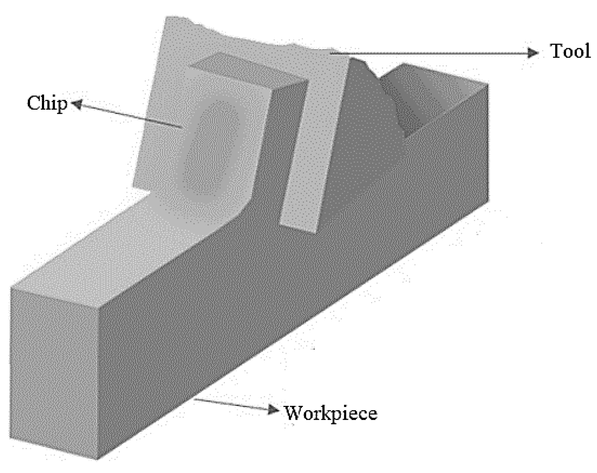
4.5. Numerical Results of Turning Operation

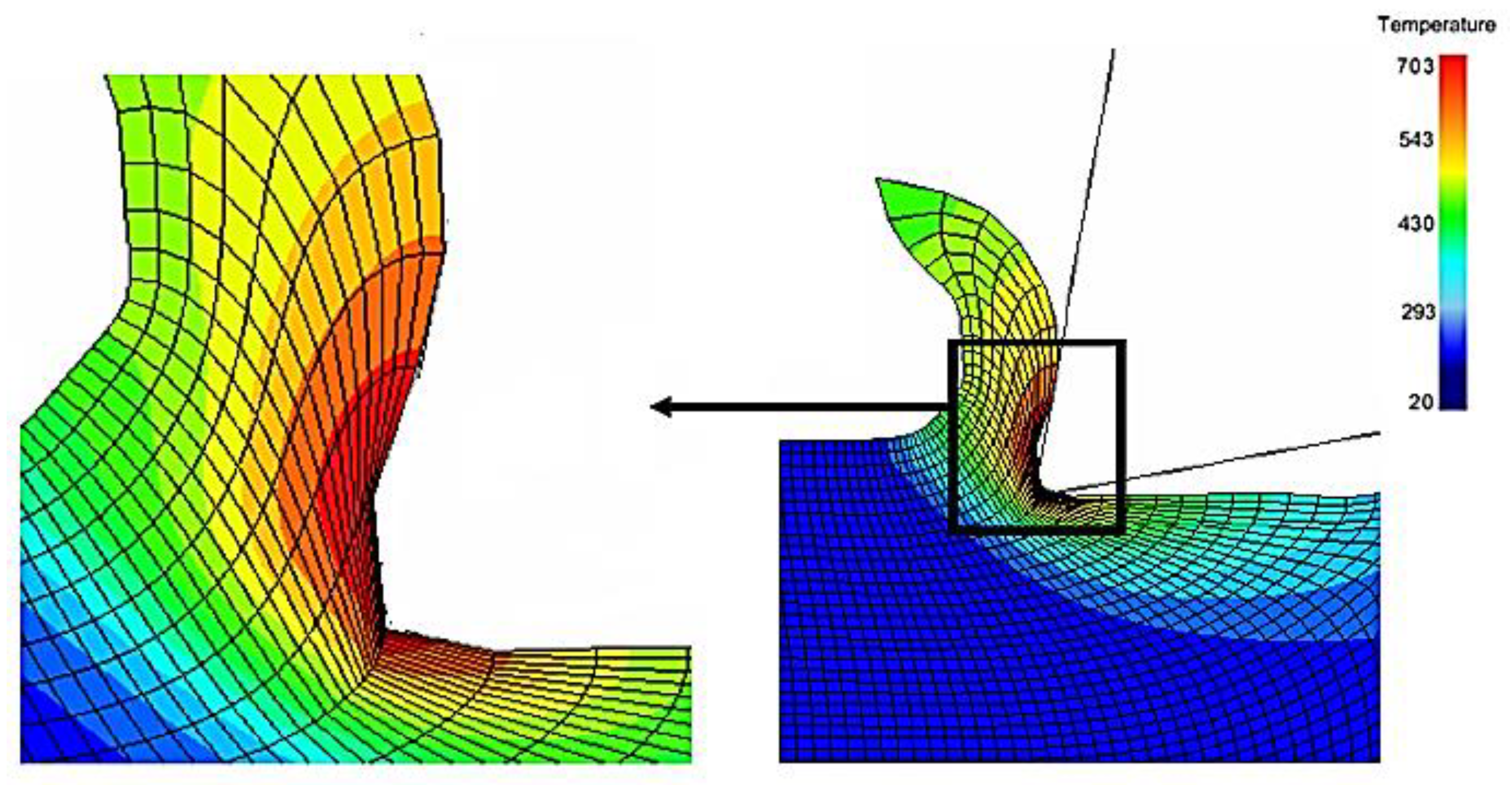
The experiment and theoretical results prove the accuracy of the turning operation’s numerical model. In the first, we illustrate in Figure 14 the computed cutting temperature distribution obtained from the numerical model.

The thermal field analysis during the cutting simulation shows that the maximum temperature is located around the tooltip, T_max = 703 °C.

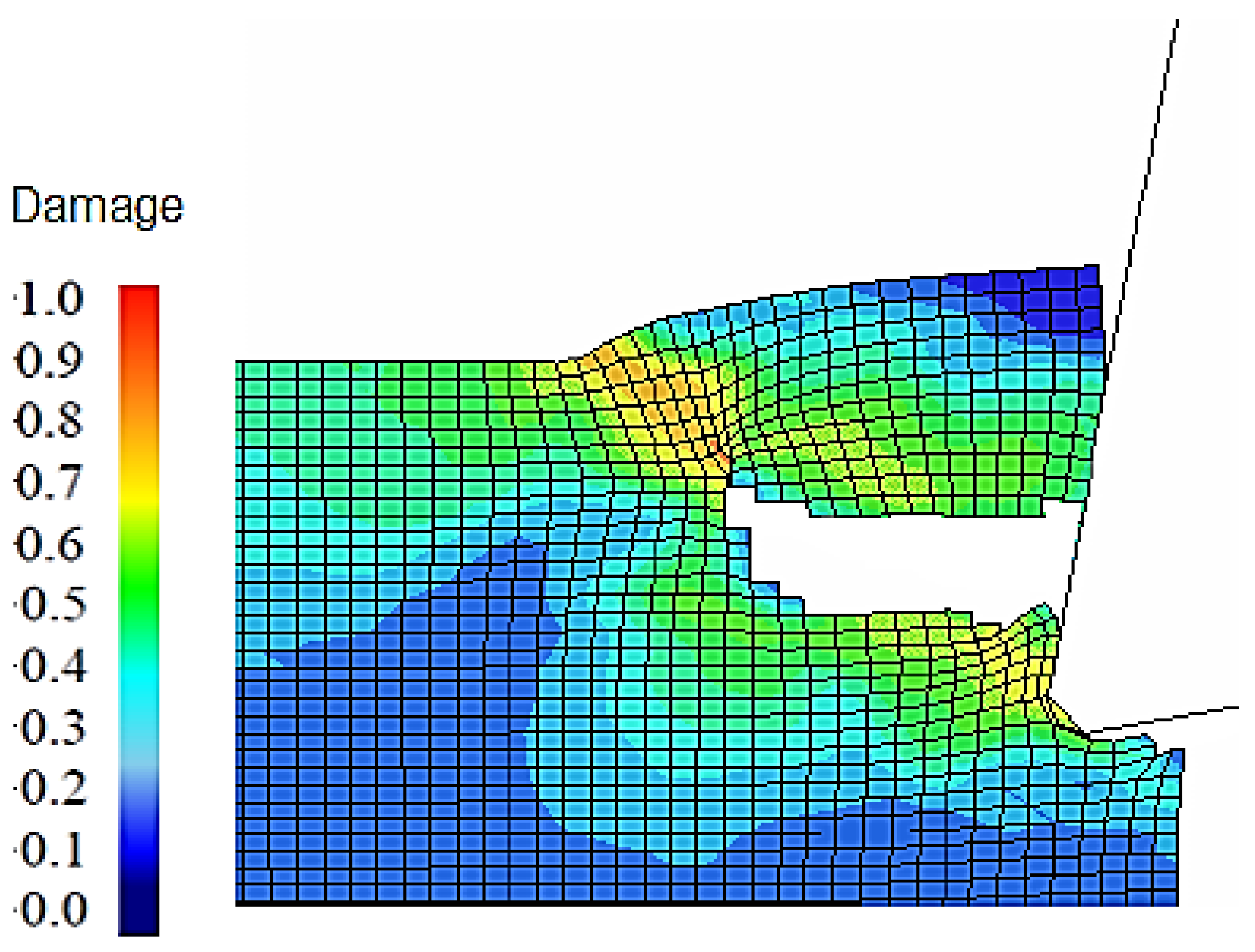
In the second, we show in Figure 15, the evolution of damage parameter in cutting model. In fact, a cutting speed Vc = 250 m/min is applied to the tool. When machining with high-cutting speed, the appearance of segmented chips happens. Using the failure model of Johnson–Cook, we can predict the discontinuous chip form.

In order to prove the accuracy of our numerical model using Johnson–Cook, we compare some numerical results with experimental and theoretical ones. The turning experiments [37] are carried out on the AISI1045 steel using a cutting speed Vc = 50 m/min and a feed rate V_f = 0.15 mm. The edge radius of the tool cutting is equal to 0.05 mm. The clearance and the rake angles are equal to 10°. A quartz-three components dynamometer was used [37] to determine tangential cutting and thrust forces Fc and Ff.

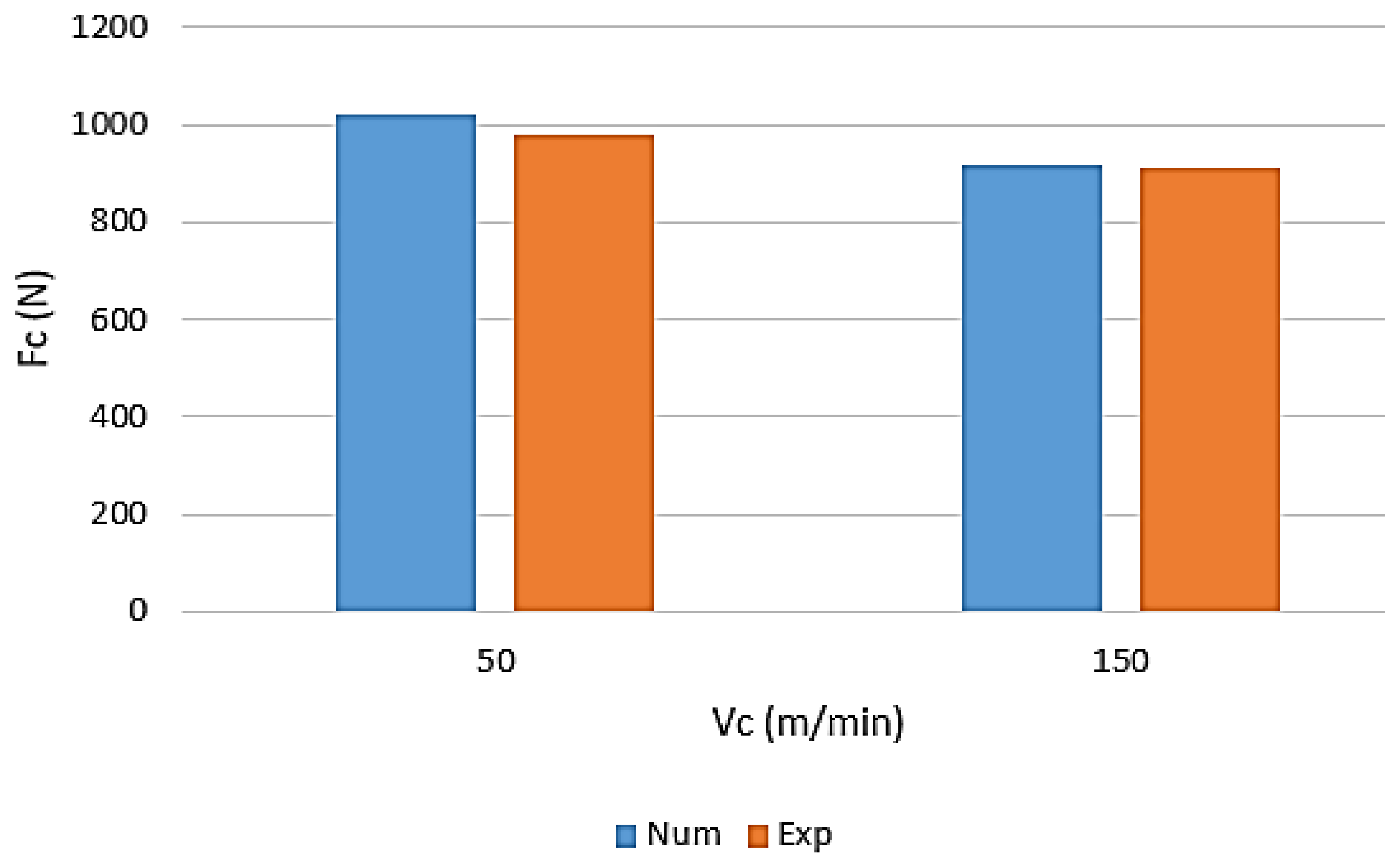
At the numerical level, we determine the chip’s cutting force and geometry, and these results may be compared to the experimental and theoretical ones as plotted in Figure 16.

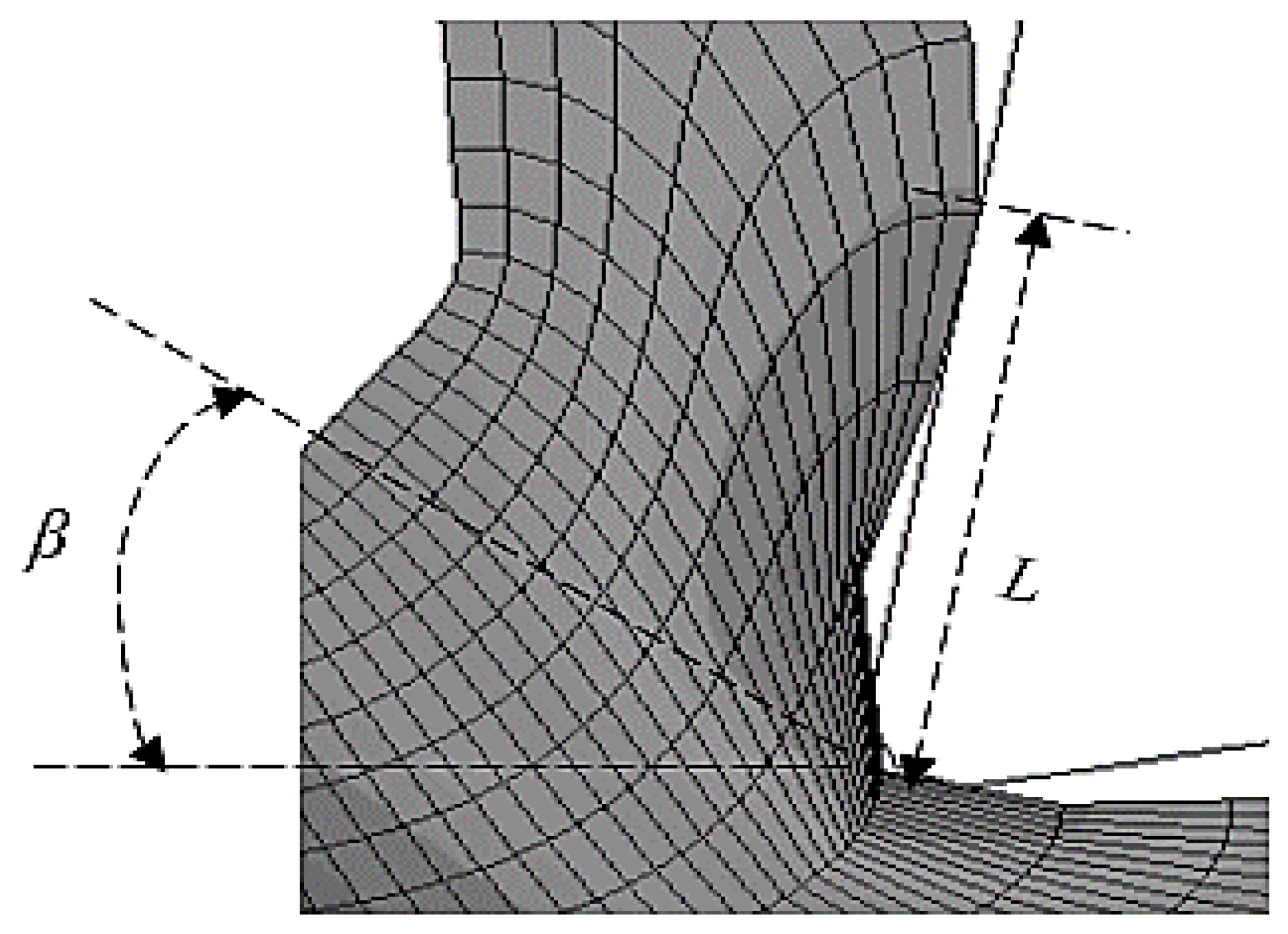
The proportionality between the total chip contact length L of and the shear angle β can be understood by looking at Figure 17.

Table 10. Numerical and experimental cutting forces, Vc = 50 m/min.

Forces (N)	Fc	Ff	R
Experimental [37]	982	615	1158
Computed with JC models	1020	570	1168
Error (%)	3.8%	7.3%	0.8%

resumes the numerical and the experimental results of cutting forces.

In addition, we illustrate in

Table 11. Chip geometries, Vc = 50 m/min.

Geometry of Chip	L (mm)	β (°)
Experimental [37]	1.1	-
Analytical [38]	-	27
Computed with JC models	1	30
Error (%)	9%	11.1%

the experimental, analytical, and numerical results of chip geometries.

The difference from the efforts of cutting does not overtake 8%. The comparison between the shear angle found by the analytical calculation [38] (β = 27°) and that computed (β = 30°) approves that the coefficients of Johnson–Cook models related to the AISI1045 are well estimated.

5. Conclusions

A thermomechanical formulation based on the Johnson–Cook model has been used to study the evolution of flow stress and failure in workpieces. In addition, the mechanical governing equations, as well as the discretization method, are presented. Moreover, accurate material damage modeling requires mechanical characterization tests. Various stress states are obtained with diverse geometry of specimens in the different tensile tests, and fracture strains are determined as a function of the triaxiality variable, strain rate, and temperature fields. The finite element analysis of sheet deep drawing and a mechanical model were developed. The uncoupled models are implemented in a finite element model simulating deep drawing as well as cutting processes. The accuracy of the model is verified by numerical simulation when predicting ductile damage in forming and cutting processes. The results show that the thermomechanical model established in this paper can accurately predict the workpiece’s behavior and failure and that it provides a numerical simulation method for describing the evolution of damage in manufacturing processes.

References

1. Lin, J.; Liu, Y.; Dean, T.A. A Review on Damage Mechanisms, Models and Calibration Methods under Various Deformation Conditions. Int. J. Damage Mech. 2005, 14, 299–319. [Google Scholar] [CrossRef]
2. Krajcinovic, D. Damage Mechanics: Accomplishments, Trends and Needs. Int. J. Damage Mech. 2000, 37, 267–277. [Google Scholar] [CrossRef]
3. Kachanov, L.M. Introduction to Continuum Damage Mechanics; Martinus Nijhoff Publisher: Dordrecht, The Netherlands, 1986. [Google Scholar]
4. Liu, K.; Jin, S.; Rui, Y.; Huang, J.; Zhou, Z. Effect of Lithology on Mechanical and Damage Behaviors of Concrete in Concrete-Rock Combined Specimen. Mathematics 2022, 10, 727. [Google Scholar] [CrossRef]
5. Benzerga, A.A.; Leblond, J.B.; Needleman, A.; Tvergaard, V. Ductile failure modeling. Int. J. Fract. 2016, 201, 29–80. [Google Scholar] [CrossRef]
6. Henseler, T.; Osovski, S.; Ullmann, M.; Kawalla, R.; Prahl, U. GTN Model-Based Material Parameters of AZ31 Magnesium Sheet at Various Temperatures by Means of SEM In-Situ Testing. Crystals 2020, 10, 856. [Google Scholar] [CrossRef]
7. Lemaitre, J. A continuous damage mechanics model for ductile fracture. J. Eng. Mater. Technol. 1985, 107, 83–89. [Google Scholar] [CrossRef]
8. Ben Said, L.; Mars, J.; Wali, M.; Dammak, F. Numerical prediction of the ductile damage in single point incremental forming process. Int. J. Mech. Sci. 2017, 131–132, 546–558. [Google Scholar] [CrossRef]
9. Bouhamed, A.; Jrad, H.; Ben Said, L.; Wali, M.; Dammak, F. A non-associated anisotropic plasticity model with mixed isotropic–kinematic hardening for finite element simulation of incremental sheet metal forming process. Int. J. Adv. Manuf. Technol. 2018, 100, 929–940. [Google Scholar] [CrossRef]
10. Bouhamed, A.; Mars, J.; Jrad, H.; Ben Said, L.; Wali, M.; Dammak, F.; Torchani, A. Identification of fully coupled non-associated-Ductile damage constitutive equations for thin sheet metal applications: Numerical feasibility and experimental validation. Thin-Walled Struct. 2022, 176, 109365. [Google Scholar] [CrossRef]
11. Gurson, A.L. Continuum Theory of Ductile Rupture by Void Nucleation and Growth: Part I-Yield Criteria and Flow Rules for Porous Ductile Media. ASME J. Eng. Mater. Technol. 1977, 99, 2–15. [Google Scholar] [CrossRef]
12. Rousselier, G. Ductile fracture models and their potential in local approach of fracture. Nucl. Eng. Des. 1987, 105, 97–111. [Google Scholar] [CrossRef]
13. Johnson, G.R.; Cook, W.H. A constitutive model and data for metals subjected to large strains, high strain rates and high temperatures. In Proceedings of the 7th International Symposium on Ballistics, The Hague, The Netherlands, 19–21 April 1983. [Google Scholar]
14. Johnson, G.R.; Cook, W.H. Fracture characteristics of three metals subjected to various strains, strain rates, temperatures and pressures. Eng. Fract. Mech. 1985, 21, 31–48. [Google Scholar] [CrossRef]
15. Xuehong, S.; Dinghua, Z.; Changfeng, Y.; Liang, T.; Xiangyu, L. Research on parameter identification of Johnson–Cook constitutive model for TC17 titanium alloy cutting simulation. Mater. Today Commun. 2022, 31, 103772. [Google Scholar]
16. Priest, J.; Ghadbeigi, H.; Ayvar-Soberanis, S.; Liljerehn, A.; Way, M. A modified Johnson-Cook constitutive model for improved thermal softening prediction of machining simulations in C45 steel. Procedia CIRP 2022, 108, 106–111. [Google Scholar] [CrossRef]
17. No, T.; Gomez, M.; Karandikar, J.; Heigel, J.; Copenhaver, R.; Schmitz, T. Propagation of Johnson-Cook flow stress model uncertainty to milling force uncertainty using finite element analysis and time domain simulation. Procedia Manuf. 2021, 53, 223–235. [Google Scholar] [CrossRef]
18. Murugesan, M.; Jung, D.W. Johnson Cook Material and Failure Model Parameters Estimation of AISI-1045 Medium Carbon Steel for Metal Forming Applications. Materials 2019, 12, 609. [Google Scholar] [CrossRef]
19. Umbrello, D.; M‘Saoub, I.R.; Outeiro, J.C. The influence of Johnson-Cook material constants on finite element simulation of machining of AISI 316L steel. Int. J. Mach. Tools Manuf. 2007, 47, 462–470. [Google Scholar] [CrossRef]
20. Patil, S.P.; Prajapati, K.G.; Jenkouk, V.; Olivier, H.; Markert, B. Experimental and Numerical Studies of Sheet Metal Forming with Damage Using Gas Detonation Process. Metals 2017, 7, 556. [Google Scholar] [CrossRef]
21. Erice, B.; Gálvez, F. A coupled elastoplastic-damage constitutive model with Lode angle dependent failure criterion. Int. J. Solids Struct. 2014, 51, 93–110. [Google Scholar] [CrossRef]
22. Slimane, A.; Bouchouicha, B.; Benguediab, M.; Slimane, S.-A. Parametric study of the ductile damage by the Gurson–Tvergaard–Needleman model of structures in carbon steel A48-AP. J. Mater. Res. Technol. 2015, 4, 217–223. [Google Scholar] [CrossRef]
23. Škrlec, A.; Klemenc, J. Estimating the Strain-Rate-Dependent Parameters of the Johnson-Cook Material Model Using Optimisation Algorithms Combined with a Response Surface. Mathematics 2020, 8, 1105. [Google Scholar] [CrossRef]
24. Schmidt, H.B.; Hattel, J.H. A local model for the thermomechanical conditions in friction stir welding. Model Sim. Mater. Sci. Eng. 2005, 13, 77. [Google Scholar] [CrossRef]
25. Sonne, M.R.; Tutum, C.C.; Hattel, J.H. The effect of hardening laws and thermal softening on modeling residual stresses in FSW of aluminum alloy 2024-T3. J. Mater. Process. Technol. 2013, 213, 477–486. [Google Scholar] [CrossRef]
26. Lestriez, P. Modélisation numérique du couplage thermomécanique endommagement en transformations finies. Appl. À La Mise En Forme 2003. [Google Scholar]
27. Leine, R.I.; Aeberhard, U.; Glocker, C. Hamilton’s Principle as Variational Inequality for Mechanical Systems with Impact. J. Nonlinear Sci. 2009, 19, 633–664. [Google Scholar] [CrossRef]
28. Liu, G.R.; Quek, S.S. The Finite Element Method: A Practical Course, 2nd ed.; Butterworth-Heinemann: Amsterdam, The Netherlands; Oxford, UK, 2013. [Google Scholar]
29. Maziar, R.; Zaidi, M.R. Deep Drawing of Sheet Metals Using the Friction-Actuated Blank Holding Technique, Rubber-Pad Forming, Processes; Woodhead Publishing: Sawston, UK, 2012; pp. 119–147. [Google Scholar]
30. Bao, Y. Prediciton of Ductile Crack Formation in Uncracked Bodies. Ph.D. Thesis, Massachusetts Institute of Technology, Cambridge, MA, USA, 2003. [Google Scholar]
31. Bi, Z. Finite Element Analysis Applications: A Systematic and Practical Approach; Academic Press: Cambridge, MA, USA, 2017. [Google Scholar]
32. Kuzmina, K.S.; Marchevsky, I.K.; Ryatina, E.P. On partitioned and monolithic coupling Lagrangian vortex methods for 2D FSI problems strategies European Conference on Computational Mechanics. In Proceedings of the 7th European Conference on Computational Fluid Dynamics (ECFD 7), Glasgow, UK, 11–15 June 2018. [Google Scholar]
33. Chocron, S.; Erice, B.; Anderson, C.E. A new plasticity and failure model for ballistic application. Int. J. Impact Eng. 2011, 38, 755–764. [Google Scholar] [CrossRef]
34. Lindgren, L.E.; Svoboda, A.; Wedberg, D.; Lundblad, M. Computational simulation of manufacturing. Comptes Rendus Mécanique 2016, 344, 209–374. [Google Scholar]
35. Nasr, M.N.A. Effects of sequential cuts on residual stresses when orthogonal cutting steel AISI 1045. Procedia CIRP 2015, 31, 118–123. [Google Scholar] [CrossRef]
36. Bridgman, P.W. Studies in Large Plastic Flow and Fracture; McGraw-Hill: New York, NY, USA, 1952. [Google Scholar]
37. Umbrello, D.; Filice, L.; Rizzuti, S.; Micari, F.; Settineri, L. On the effectiveness of finite element simulation of orthogonal cutting with particular reference to temperature prediction. J. Mater. Process. Technol. 2007, 189, 284–291. [Google Scholar] [CrossRef]
38. Oxley, P.L.B.; Shaw, M.C. Mechanics of Machining: An Analytical Approach to Assessing Machinability. ASME J. Appl. Mech. 1990, 57, 253. [Google Scholar] [CrossRef] [Green Version]
Figure 1. Conventional deep-drawing process [29].
Mathematics 10 03555 g001
Figure 2. Conventional curves of specimens with respect to the rolling direction 0, 45, and 90°.
Mathematics 10 03555 g002
Figure 3. Logarithm curve of the Johnson–Cook hardening model.
Mathematics 10 03555 g003
Figure 4. (a) Smooth sheet specimen; (b) Notched sheet specimens.
Mathematics 10 03555 g004
Figure 5. Relationship plot of strain to fracture and stress triaxiality: Flat specimens made of DC01 steel.
Mathematics 10 03555 g005
Figure 6. Die, blank-holder, and punch for the car fuel tank.
Mathematics 10 03555 g006
Figure 7. First test: Experimental and Numerical results of car fuel tank deep drawing.
Mathematics 10 03555 g007
Figure 8. Second test: Experimental and Numerical results of car fuel tank deep drawing.
Mathematics 10 03555 g008
Figure 9. Conventional curve of AISI1045 steel.
Mathematics 10 03555 g009
Figure 10. Fitting curve ln(σ−A) in function of ln(ε).
Mathematics 10 03555 g010
Figure 11. (a) Smooth round specimen; (b) Notched round specimen.
Mathematics 10 03555 g011
Figure 12. Relationship plot of strain to fracture and stress triaxiality: Flat specimens made of AISI1045 material.
Mathematics 10 03555 g012
Figure 13. Modeling of turning operation.
Mathematics 10 03555 g013
Figure 14. Temperature distribution with Vc = 50 m/min.
Mathematics 10 03555 g014
Figure 15. Distribution of damage parameter D.
Mathematics 10 03555 g015
Figure 16. Computed tangential cutting force Fc (N) in function of cutting speed Vc (m/min).
Mathematics 10 03555 g016
Figure 17. Total chip contact length L and angle of shear β.
Mathematics 10 03555 g017