Elementary Cellular Automata as Invariant under Conjugation Transformation or Combination of Conjugation and Reflection Transformations, and Applications to Traffic Modeling

Abstract

This paper develops the analysis of properties of the cellular automata class introduced by the authors. It is assumed that the set of automaton cells is finite and forms a closed lattice, and there are two states for each automaton cell. We consider a new concept. This concept is the average velocity of a cellular automaton, which characterizes the average intensity of changes in the states of the automaton’s cells for a given initial state. The automaton velocity is equal to 1 if the state of any cell changes at each step. The spectrum of average velocities of a cellular automaton is the set of average velocities for different initial states. Since the state space is finite, the automaton, starting from a certain moment of time, is in periodically repeating states of a cycle, and thus, the research of the velocity spectrum is related to the problem of studying the set of the automaton cycles. For elementary cellular automata, the introduced class consists of a subclass of automata such that the conjugation trasformation of an automaton is the automaton itself (Subclass A) or the reflection of the automaton (Subclass B). For this class, it is proved that the spectrum of the automaton contains the value $v_0$ if and only if the spectrum of the complementary automaton contains the value $1-v_0$ (the sum of the index of elementary cellular automaton and the complementary automaton is 255). For automata of Subclasses A and B, the set of cycles and the velocity spectrum are studied. For Subclass A, a theorem has been proved such that in accordance with this theorem, if two automata complementary to each other start evolving in the same initial state, then the sum of their average velocities is equal to 1. This theorem for Subclass A is generalized to cellular automata, invariant under the conjugation transformation, of more general type than elementary automata. Generalizations of the theorem have been given for the class of one-dimensional cellular automata with a neighborhood containing $2r+1$ cells (the next state of the cell depends on the present states of this cell, r cells on the left and r cells on the right) and for some traditionally considered classes of two-dimensional automata. Some elementary cellular automata belonging to the class considered in the paper can be interpreted as transport models. The properties of the spectra for these automata are studied and compared with the properties of elementary cellular automata not invariant under the considered transformations and can also be interpreted as transport models. The analytical results obtained for these simple models can be used to study the qualitative properties and limiting behavior of more complex transport models.

1. Introduction

The concept of a cellular automata was introduced in [1,2,3]. Methods of cellular automata are widely applied in computer science, biology, physics, etc.

For a cellular automaton, the next state of each cell depends on the present states of this cell and some adjacent cells. For an elementary cellular automaton (ECA) [4], the set of cells is a closed or infinite one-dimensional lattice, and the next state of a cell depends on this cell and the states of two adjacent cells at the present moment. There exist only two states for a cell of an elementary cellular automata. These states are 0 and 1. There exist 256 elementary cellular automata.

The concepts of conjugation and reflection transformations are considered in [5], where a related table is presented. These transformations were also considerd in [6]. The set of cellular automata is divided into 88 subsets such that each of these subsets contains one, two, or four elementary cellular automata. Any two automata belonging to the same subset may be obtained from each other by the conjugation transformation, or the reflection transformation, or by the combination of the conjugation and reflection transformations.

In [7], a classification of the elementary cellular automata was introduced such that the set of elementary cellular automata is divided into 46 subsets. Automata of the same class can be obtained by permutations of the neighborhood.

The concept of complementary automaton was introduced in [8].

Some classifications of elementary cellular automata were introduced in [6,8,9,10]. In [11], different classifications of elementary cellular automata are overviewed. Suppose an elementary cellular automaton is defined on a closed lattice of n cells. Then, from a moment, a sequence of cellular automaton states is repeated (cycle, or limit cycle). In [12], for a cellular automaton defined on a closed lattice, the concept of the automaton velocity has been introduced.

In [12,13], elementary cellular automata were considered such that these automata can be interpreted as binary closed chains. The concept of a binary closed chain was introduced in [13,14,15]; see Figure 1. The binary chains belong to the class of dynamical systems called the Buslaev contour networks (BCN). This class was introduced in [14] to develop traffic mathematical models with a network structure. The binary chain contains circumferences (contours) with common nodes. There are two cells and a particle in any contour. Particles on neighborhood contours cannot cross a common node simultaneously; the competition rule is the left-priority rule. A contour is in the state 0 if the particle is in the lower cell, and the contour is in the state 1 if the particle is in the upper cell. A contour corresponds to a cell of a cellular automaton. The next state of a contour at time $t+1$ depends on the states of this contour and two adjacent contours at time $t.$

In versions of discrete contours networks, particles move through the contours under the rule ECA 184, see Figure 2 (Left), or ECA 240, see Figure 2 (Right). The rule ECA 240 corresponds to the cluster movement. The concept of cluster movement in traffic models was introduced in [16]. At any time, each cell is vacant or the cell is occupied by a particle. Any cell of a cellular automaton is in the state 0 if the corresponding cell of the model is vacant, and the automaton state is 1 if the corresponding cell of the model is occupied. In the case of movement under the rule 184, a particle moves onto a cell in the direction of movement if the cell ahead is vacant. In the case of movement under the rule 240, at any step, each particle moves onto a cell in the direction of movement.

In [17,18], analytical results for a traffic model equivalent to ECA 184 have been obtained. This model is a simple version of the Nagel–Schreckenberg model [19]. In [20], a traffic model in which particles move under a two-dimensional counterpart of the rule ECA 184 was introduced.

ECA 184 and ECA 240 are numbers conserving cellular automata [21,22].

In [23], a traffic model based on a stochastic version of ECA 184 was studied. Different approaches exist to introduce a stochastic version of an elementary cellular automaton. In [24] stochastic versions conserving mass were introduced for ECA 184 and ECA 240.

ECA 136 and ECA 252 can be also used for traffic modeling [25].

The paper [26] has introduced a graph cellular automaton with a variable configuration of cells. It is noted in [26] that this automaton may be used as models of complex systems, in particular, transport networks.

This paper considers a class of elementary cellular automata such that the conjugation transformation or the combination of the conjugation and reflection transformations of an automaton is the same automaton. The number of cells of automaton is finite, and the cells form a closed chain. We study closed trajectories in the automaton state space (cycles) and the rate of state transitions called the average velocity of the cycle or the average velocity of cellular automaton for the prescribed initial state. By definition, the average velocity is equal to the average number of cell state transitions per a time unit. We have proved for 20 of 24 automata of the considered class that if for an automaton belonging to the considered class, there is the value $v_0$ in the spectrum of average velocities; then, there is the value $1-v_0$ in the spectrum of the complementary automaton. For the other four automata of the class, this statement is formulated as a hypothesis. We study two subclasses of the considered class. Subclass A consists of the elementary cellular automata invariant under the conjugation transformation. Subclass B consists of the elementary cellular automata non-invariant under the conjugation transformation and invariant under the combination of the conjugation and reflection transformations. For considered automata, theorems characterizing the spectrum of velocities have been proved.

Section 3 studies the class of elementary cellular automata invariant under the conjugation transformation (Subclass A). Section 4 studies the spectrum the class of elementary cellular automata non-invariant under the conjugation transformation and invariant under the combination of the conjugation and reflection transformations (Subclass B). Section 5 considers relations between the classes of ECA considered in Section 3 and Section 4 and the classes in classifications considered in [6,8,9,10,11]. Section 6 considers interpretations of concepts related to cellular automata in terms of contour networks and traffic models.

This paper is an extended version of the conference paper [27]. The paper formulates Theorems 4, 6, 9–13, 17, 18, and they have been proved, such that these theorems are not found in [27]. Theorems 4 and 6 refer to the application of permutations in neighborhoods of elementary cellular automata that are invariant under the conjugation transformation. Such permutations were not considered the conference paper. Theorems 9–13 refer to the spectrum of average velocities of elementary cellular automata that are invariant under the conjugation transformation. In [27], only a general theorem was formulated and proved on the relationship between the spectra of complementary elementary cellular automata that are invariant under the conjugation transformation. In this paper, we also study the form of the spectra of specific elementary cellular automata belonging to this subclass. Theorems 17 and 18 refer to the generalization of the theorem on the relationship between the spectra of elementary cellular automata complementary to each other, invariant under the conjugation transformation, respectively, to one-dimensional cellular automata with a more general form of neighborhoods than for elementary automata and to two-dimensional automata. In [27], such classes of cellular automata were not considered. The contents of Section 7 and most of Section 8 are also new.

2. Problem Formulation

Assume that there is a one-dimensional closed sequence of cells. Denote by n the number of cells. At each moment $t=0,1,2,\dots ,$ any cell is in the state 0 or 1. At time $t+1,$ the cell i is in the state depending on the states of $i-1$ (subtraction modulo $n),$ $i,$ and $i+1$ (addition modulo $n)$ a at time $t,$ $i=0,1,\dots ,n-1.$ An elementary cellular automaton (ECA) is defined by the table

$$111\to a_7,110\to a_6,101\to a_5,100\to a_4,011\to a_3,010\to a_2,001\to a_1,000\to a_0,$$

where $a_i=0\vee 1,$ $i=0,\dots ,7.$

Let the cell i be in the state $x_i\left(t\right)$ at time $t.$ Denote by $x^t=x\left(t\right)=(x_0\left(t\right),x_1\left(t\right),\dots ,$ $x_{n-1}\left(t\right))$ the state of the automaton at time $t.$

The index N of an elementary cellular automaton is equal to

$$N=\sum _{i=0}^7{a}_i·2^i.$$

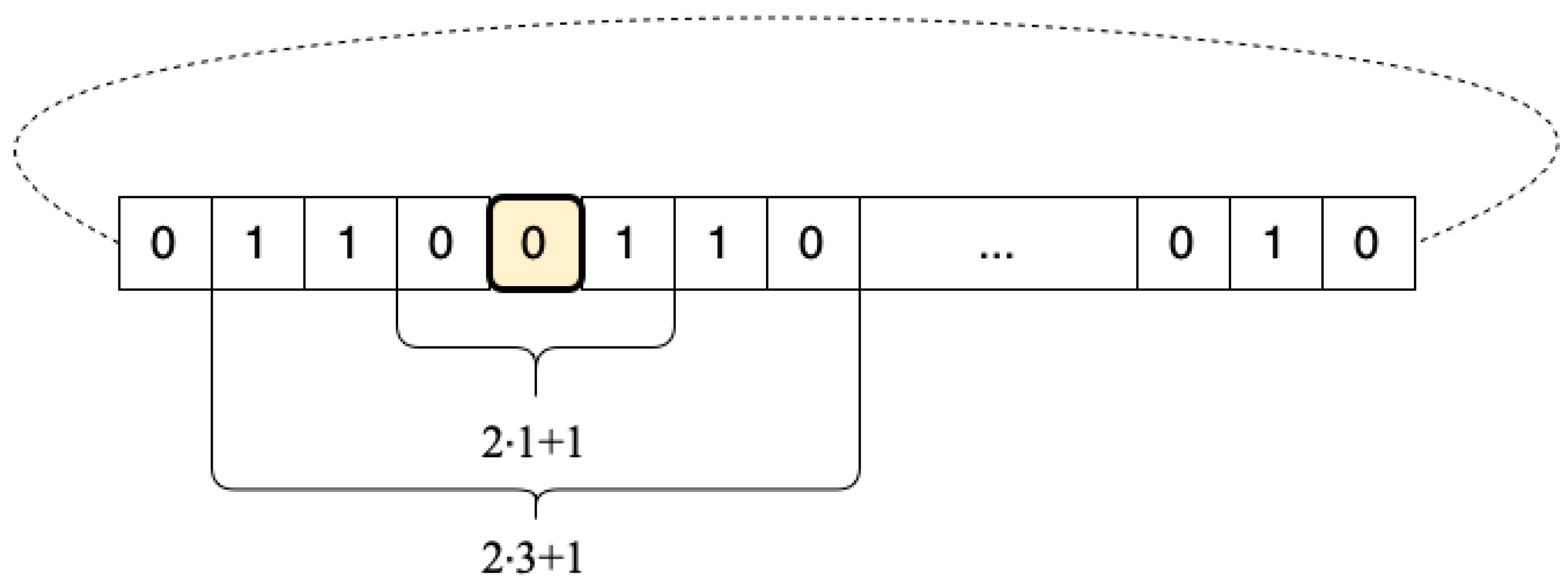
We characterize the next state of an elementary cellular automaton by the function $f$:

$$x_i^{t+1}=f(x_{i-1}^t,x_i^t,x_{i+1}^t).$$

The variation of the state $x=(x_0,x_1,\dots ,x_{n-1})$ is defined as

$$\mathrm{var}\left(x\right)=\frac{1}{2}\left(|x_0-x_{n-1}|+\sum _{i=1}^{n-1}|x_i-x_{i-1}|\right).$$

From a moment, a sequence of automaton states is repeated (a cycle). This sequence depends on the initial state $x^0$ of the automaton.

Let the value $\Delta x^t$ be defined as the following.

$$\Delta x^t=\frac{1}{n}\sum _{i=0}^{n-1}|x_i^t-x_i^{t+1}|.$$

Then, the value

$$v\left(x^{t_0}\right)=\frac{1}{T}\sum _{t=t_0}^{t_0+T-1}\Delta x^t,$$

depending on the initial state $x^{t_0}$, is called the average velocity of cycle with the period $T.$

By definition, the spectrum of cellular automaton average velocities is the set of the average velocities for different initial states.

A state x of an elementary cellular automaton is called absorbing if, from the condition $x\left(t_0\right)=x$ it follows that at any time $t\ge t_0,$ the automaton is in the state x.

Suppose the state x of an elementary cellular automaton satisfies the following condition. If at time $t_0,$ the automaton is in the the state $x,$ then the automaton is in the state x at any $t\ge t_0.$ In this case, the state x is called absorbing. Obviously, $v\left(x^0\right)=0$ for a absorbing state $x_0.$

By definition, a cluster of zeros (0-cluster) is a set of zeros in neighboring cells. There are ones in positions between two 0-clusters. A definition of a cluster of ones (1-cluster) is analogous. A cluster of the length k is the cluster containing k zeros or k ones.

If the state vector contains only ones or only zeros, then the state variation equals 0. If the vector k contains clusters of zeros and k clusters of ones, then the state variation equals $k.$

Suppose that ${\overline{x}}_i=1,$ if $x_i=0,$ and ${\overline{x}}_i=0,$ if $x_i=1.$

We use the following definitions [5,7,10].

The elementary cellular automaton defined by the rule $f_i,$ $i=1,\dots ,8,$ if, for any $x_{i-1},$ $x_i,$ $x_{i+1}$ (equal to 0 or 1), the following condition holds:

$$f_i(x_{i-1},x_i,x_{i+1})=\overline{f({\overline{x}}_{i-1},{\overline{x}}_i,{\overline{x}}_{i+1})},i=1,$$

$$f_i(x_{i-1},x_i,x_{i+1})=f(x_{i+1},x_i,x_{i-1}),i=2,.$$

$$f_i(x_{i-1},x_i,x_{i+1})=\overline{f({\overline{x}}_{i+1},{\overline{x}}_i,{\overline{x}}_{i-1})},i=3,$$

$$f_i(x_{i-1},x_i,x_{i+1})=f(x_{i-1},x_{i+1},x_i),i=4,$$

$$f_i(x_{i-1},x_i,x_{i+1})=f(x_i,x_{i-1},x_{i+1}),i=5,$$

$$f_i(x_{i-1},x_i,x_{i+1})=f(x_i,x_{i+1},x_{i-1}),i=6,$$

$$f_i(x_{i-1},x_i,x_{i+1})=f(x_{i+1},x_{i-1},x_i),i=7.$$

The rule $f_1$ is called the conjugation transformation. The rule $f_2$ is called the reflection transformation. The rule $f_3$ is called the combination of conjugation and reflection transformations. The rule $f_4$ is called permutation ${\pi }_2$ in neighborhood. The rule $f_5$ is called the permutation ${\pi }_2$ in neighborhood. The rule $f_6$ is called the permutation ${\pi }_3$ in neighborhood. The rule $f_7$ is called the permutation ${\pi }_4$ in neighborhood.

We say that the reflection of a cellular automaton is obtained by the application of the permutation ${\pi }_5$ to this automaton.

We say that the result is obtained by the application of the permutation ${\pi }_0$ to this automaton itself.

The automaton, defined by the rule $f_8,$ is called complementary to the automaton defined by the rule f if, for any $x_{i-1},$ $x_i,$ $x_{i+1},$

$$f_8(x_{i-1},x_i,x_{i+1})=\overline{f(x_{i-1},x_i,x_{i+1})}.$$

The sum of the indices of elementary cellular automata complementary to each other equals 255.

We consider the class of elementary cellular automata invariant under the conjugation transformation or the combination of the conjugation and the reflection transformations. We study the following two subclasses of the class.

Subclass A consists of the elementary cellular automata such that the results of application of the conjugation transformation to an automaton are the same automaton (the elementary cellular automata invariant under the conjugation transformation). This class contains 16 automata.

Subclass B consists of the elementary cellular automata such that the results of application of the conjugation transformation to an automaton are the reflection of this automaton (the elementary cellular automata invariant under the combination of conjugation and reflection transformations), and the automaton does not belong to subclass A. This subclass contains eight automata.

Note that six automata belonging to Subclass A are invariant under both the conjugation transformation and the combination of the conjugation and reflection transformations.

We study the spectrum of average velocities of automata belonging to the considered class. We shall prove the following. Suppose an automaton belongs to the considered class. Then, the complementary automaton also belongs to this class, and if the spectrum of one of these supplementary to each other automata contains value $v_0,$ then the other automaton contains the value $1-v_0.$ We prove other theorems for automata of the considered classes.

3. Elementary Cellular Automata Invariant under Conjugation Transformation

Theorem 1.

Suppose the elementary cellular automaton N belongs to Subclass A. Assume that the initial state is the same for these automata. Then, the sum of the average velocity of this automaton and the average velocity of the complementary automaton $255-N$ equals 1.

Proof. 

Suppose $x=(x_1,\dots ,x_n).$ The state $\overline{x}=({\overline{x}}_1,\dots ,{\overline{x}}_n)$ is called complementary to the state $x.$ If at time $t,$ the automata ECA N and ECA $255-N$ are in the same state, then at time $t+1,$ these automata will be in states complementary to each other. If at time $t,$ the automata ECA N and ECA $255-N$ are in states complementary to each other, then, taking into account that the automaton ECA N is conjugation of itself, we have that at time $t+1,$ the automata ECA N and ECA $255-N$ will be in the same state. Therefore, if $x^0$ is the initial state of both the automata and, at time $t,$ ECA N is in the state $x^t,$ then, at time $t,$ ECA $255-N$ is in the state ${\overline{x}}^t$ for $t=1,3,5,\dots ,$ and ECA $255-N$ is in the state $x^t$ for $t=2,4,6,\dots$. From this, Theorem 1 follows. □

Theorem 2.

Suppose an elementary cellular automaton N belongs to Subclass A and there is a value $v_0$ in the spectrum of average velocities for ECA $N.$ Then, for the complementary elementary cellular automaton $255-N,$ there is the value $1-v_0$ in the spectrum of average velocities if and only if, for the elementary cellular automaton $N,$ there is the value $v_0$ in the spectrum.

Theorem 2 is a corollary of Theorem 1.

Theorem 3.

The spectrum of average velocities is the same for an elementary cellular automaton $N,$ the conjugation of ECA $N,$ the reflection of ECA $N,$ and the automaton obtained from the ECA N by the combination of the conjugation transformation and reflection transformation.

Theorem 4.

Suppose that the elementary cellular automaton N belongs to Subclass A. Let ECA $N^{\prime }$ be a permutation ${\pi }_1,$ ${\pi }_2,$ ${\pi }_3,$ or ${\pi }_4$ of ECA $N.$ Then, ECA $255-N^{\prime }$ is a permutation ${\pi }_1,$ ${\pi }_2,$ ${\pi }_3,$ or ${\pi }_4$ of the elementary cellular automaton $255-N$, respectively.

Theorems 3 and 4 are obvious.

Subclass A contains just 16 automata. They are ECA 015, ECA 023, ECA 043, ECA 051, ECA 077, ECA 085, ECA 105, ECA 113, ECA 142, ECA 150, ECA 170, ECA 178, ECA 204, ECA 212, ECA 232, and ECA 240.

Theorem 5.

If ECA N belongs to Subclass A, then Subclass A contains the automaton that is obtained from ECA N by the conjugation transformation, the reflection transformation, or a combination of conjugation and reflection transformations.

We can prove Theorem 5 using the tables of the conjugation and reflection equivalence [5].

Theorem 6.

Suppose ECA N belongs to Subclass A. Then, each of the permutations ${\pi }_1,$ ${\pi }_2,$ ${\pi }_3,$ and ${\pi }_4$ for the rule ECA N belongs to Subclass A.

Proof. 

Permutations ${\pi }_1,$ ${\pi }_2,$ ${\pi }_3,$ and ${\pi }_4$ of ECA 015 are ECA 015, ECA 051, ECA 051, and ECA 085, respectively. Hence, any of the permutations ${\pi }_1,$ ${\pi }_2,$ ${\pi }_3,$ and ${\pi }_4$ of ECA 015 is an automaton belonging to Subclass A. Each of the permutations ${\pi }_1,$ ${\pi }_2,$ ${\pi }_3,$ and ${\pi }_4$ of the rule ECA 023 is the rule ECA 023 itself. Permutations ${\pi }_1,$ ${\pi }_2,$ ${\pi }_3,$ and ${\pi }_4$ of the rule ECA 043 are the rules ECA 077, ECA 043, ECA 113, and ECA 077 respectively. Permutations ${\pi }_1,$ ${\pi }_2,$ ${\pi }_3,$ and ${\pi }_4$ of the rule ECA 051 are ECA 085, ECA 015, ECA 085, and ECA 015, respectively. Permutations ${\pi }_1,$ ${\pi }_2,$ ${\pi }_3,$ and ${\pi }_4$ of the rules ECA 077 are the rules ECA 043, ECA 113, ECA 043, and ECA 113, respectively. Permutations ${\pi }_1,$ ${\pi }_2,$ ${\pi }_3,$ and ${\pi }_4$ of the rule ECA 085 are the rules ECA 051, ECA 085, ECA 015, and ECA 051, respectively. Each of the permutations ${\pi }_1,$ ${\pi }_2,$ ${\pi }_3,$ and ${\pi }_4$ of the rule ECA 105 is the rule ECA 105 itself. Permutations ${\pi }_1,$ ${\pi }_2,$ ${\pi }_3,$ and ${\pi }_4$ of the rule ECA 113 are the rules ECA 113, ECA 077, ECA 077, and ECA 043, respectively. Thus, each of the permutations ${\pi }_1,$ ${\pi }_2,$ ${\pi }_3,$ and ${\pi }_4$ of any automaton belonging to Subclass A is also an any automaton belonging to Subclass A. Theorem 6 has been proved. □

Theorem 7.

There are $[n/2]+1$ values in the spectrum of average velocities for ECA 015 and ECA 085. These values are $1-2k/n,$ $k=0,1,\dots ,[n/2]$ $\left(\right[a]$ is the integral part of $a).$

Theorem 8.

There are $[n/2]+1$ values in the spectrum of average velocities for ECA 170 and ECA 240. These values are $2k/n,$ $k=0,1,\dots ,[n/2].$

Theorems 7 and 8 are proved in [13].

Theorem 9.

If the number n is odd, then, for ECA 023, the there is only the value 1 in the spectrum of average velocities. If the number n is even, then, for ECA 023, the spectrum contains only the values 0 and 1.

Proof. 

The table of the rule ECA 023 is

$$111\to 0,110\to 0,101\to 0,100\to 1,011\to 0,010\to 1,001\to 1,000\to 1.$$

If the number n is even, then the state $(0,1,0,1,\dots ,0,1)$ is absorbing, and the spectrum contains the value 0.

The state $(0,\dots ,0)$ and $(1,\dots ,1)$ belongs to a cycle with period 2 and velocity 1.

If the vector of state contains both 0-clusters and 1-clusters and at least one 0-cluster of the length greater than 1 or 1-cluster of the length greater than 1, then, at each step, the variation decreases at least by 1. Thus, from any initial state, the automaton results in the state $(0,\dots ,0)$ or $(1,\dots ,1),$ or (for an even $n),$ or a state containing only 0-clusters of length 1 and 1-clusters of length 1. This completes the proof. □

Theorem 10.

If n is odd, then, for ECA 232, there only the value 0 in the spectrum of average velocities. If n is even, then, for ECA 232, the spectrum of average velocities contains only the values 0 and 1.

Theorem 10 follows from Theorems 2 and 9.

Theorem 11.

There is only the value 1 in the spectrum of the average velocities for ECA 051. There is only the value 0 in the spectrum of the average velocities for ECA 204.

Theorem 11 follows from that, for ECA 051, the state of any cell changes at each step, and, for ECA 204, the state of the automaton does not change at any step.

Theorem 12.

There are only the values 0 and 1 in the spectrum of the average velocities for ECA 077.

Proof. 

The table of the rule ECA 077 is

$$111\to 0,110\to 1,101\to 0,100\to 0,011\to 1,010\to 1,001\to 0,000\to 1.$$

In accordance with this rule, the state of a cell changes if and only if this cell, the adjacent cell on the left, and the adjacent cell on the right are in the same state. The states $(0,\dots ,0)$ and $(1,\dots ,1)$ belong to a cycle with the average velocity 1 and period 2. Suppose there are both zeros and ones in the vector. If the vector of state contains no clusters of zeros or ones of length greater than 2, then no cell changes its state. Suppose at the state vector $x\left(t\right)$, there is a 0-cluster (1-cluster) of length $l\ge 3$. Then, the vector $x(t+1)$ will contain two 0-clusters (1-clusters) of length 1 and a 1-cluster (0-cluster) of length $l-2$ between them. The states of cells not belonging to clusters of length not greater than 2 do not change. Therefore, the length of the longest cluster decreases at each step until the maximum length becomes not greater than 2, and, at any step, there are both 0-clusters and 1-clusters. Therefore, from any state except the states $(0,\dots ,0)$ and $(1,\dots ,1),$ the automaton results in an absorbing state. From this, Theorem 12 follows. □

Theorem 13.

There are only the values 0 and 1 in the spectrum of the average velocities for ECA 178.

Theorem 13 follows from Theorems 2 and 12.

4. Elementary Cellular Automata Invariant under Combination of Conjugation and Reflection Transformations

In Section 4, theorems are proved, and a hypothesis is formulated for cellular automata invariant under the combination of the conjugation and reflection transformations (Subclass B).

Theorem 14.

There exist $[n/2]+1$ values in the spectrum of the average velocities for ECA 029 and ECA 071. These values are $1-2k/n,$ $k=0,1,2,\dots ,[n/2]$.

Theorem 15.

There are $[n/2]+1$ values in the spectrum of the average velocities for ECA 184 and ECA 226. These values are $2k/n,$ $k=0,1,2,\dots ,[n/2]$.

Theorems 14 and 15 were proved in [13].

Subclass B contains just eight automata ECA 029, ECA 057, ECA 071, ECA 099, ECA 156, ECA 184, ECA 198 and ECA 226.

Theorem 16.

Assume that ECA N belongs to Subclass B. Then, Subclass B contains the automaton obtained from ECA N by the conjugation or reflection transformation, or the combination of the conjugation and reflection transformations.

We can prove Theorem 16 using the table of the conjugation equivalence represented in [5].

Hypothesis 1.

Assume that an elementary cellular automaton N belongs to Subclass B and the spectrum of average velocities contains the value $v_0.$ Then, for the complementary automaton $255-N,$ there is the value $1-v_0$ in the spectrum of average velocities.

From Theorems 14 and 15, it follows that for the pairs of cellular automata complementary to each other, ECA 029, ECA 226 and ECA 071, ECA 184, the statement holds. If the statement holds for the pair ECA 057, ECA 198, then it holds for the pair ECA 099, ECA 156 because ECA 099 is the conjugation of ECA 057, and ECA 156 is the conjugation of ECA 198.

For ECA 057, the spectrum of velocities consists of the following values: 1 for $n=2;$ 2/3 and 1 for $n=3;$ 1 for $n=4;$ 4/5, 1 for $n=5;$ 2/3, 1 for $n=6;$ 5/7, 6/7, 1 for $n=7;$ 3/4, 1 for $n=8.$

For ECA 198, the spectrum of velocities consists of the following values: 0 for $n=2;$ 0 and 2/3 for $n=3;$ 0 for $n=4;$ 0, 4/5 for $n=5;$ 0, 1/3 for $n=6;$ 0, 1/7, 2/7 for $n=7;$ 0, 1/4 for $n=8.$

Thus, for $n\le 8,$ the automata ECA 057, ECA 198 satisfy the statement of Hypothesis 1.

The following example shows that the statements analogous to Theorem 6, in general, are not true for Subclass B.

Example 1.

The rule ECA 184 belongs to Subclass B. The rule ECA 216 is obtained by the permutation ${\pi }_1$ of the rule ECA 184. The rule ECA 039 is supplementary to the rule 216. The rules ECA 039, ECA 216 belong to neither Subclass A nor Subclass B.

The table of the rule ECA 216 is

$$111\to 1,110\to 1,101\to 0,100\to 1,011\to 1,010\to 0,001\to 0,000\to 0.$$

The table of the rule ECA 039 is

$$111\to 0,110\to 0,101\to 1,100\to 0,011\to 0,010\to 1,001\to 1,000\to 1.$$

Suppose $n=3$ and $(0,0,1)$ is the initial state of ECA 039. Then, we have the following sequence of transitions:

$$(0,0,1)\to (0,1,1)\to (1,0,0)\dots$$

We have a cycle with period 6 and the average velocity $v_0=2/3.$ However, the spectrum of average velocities for ECA 216 does not contain $1-v_0=1/3.$ Indeed, we have for ECA 216

$$(0,0,0)\to (0,0,0),$$

$$(0,0,1)\to (1,0,0),$$

$$(0,1,1)\to (0,1,1),$$

$$(1,1,1)\to (1,1,1).$$

Thus, for ECA 216, the spectrum of average velocities contains only the values 0 and 2/3.

5. Generalization for Cellular Automata with Neighborhoods Containing $\mathbf{2}\mathit{r}+\mathbf{1}$ Cells

This section generalizes Theorem 1 for one-dimensional cellular automata with neighborhoods containing $2r+1$ cells, Figure 3.

In [9], a generalization of elementary cellular automata has been introduced. For this generalization, at any time each state is in one of k states, and the state of a cell at time $t+1$ depends on the state of this cell and the states of the cells at a distance up to r on both sites:

$$x_i^{t+1}=f(x_{i-r}^t,x_{i-r+1}^t,\dots ,x_i^t,\dots ,x_{i+r}^t)$$

Suppose a cellular automaton evolves on a closed lattice containing n cells. The definitions of the average velocity and the spectrum of average velocities are the same as for elementary cellular automata.

We shall give the following definition. The automaton with the rule $f_2$ is called complementary for the the automaton with the rule $f_1$ if, for any $x_{i-r},$ $x_{i-r+1}\dots ,x_i,\dots ,x_{i+r},$

$$f_1(x_{i-r},x_{i-r+1},\dots ,x_i,\dots ,x_{i+r})=\overline{f_2(x_{i-r},x_{i-r+1},\dots ,x_i,\dots ,x_{i+r})}.$$

We shall give the definition of Class A. A cellular automaton with rule f belongs to Class A if and only if, for any $x_{i-r},$ $x_{i-r+1}\dots ,x_i,\dots ,x_{i+r}$ (addition and subtraction modulo $n),$

$$f(x_{i-r},x_{i-r+1},\dots ,x_i,\dots ,x_{i+r})=\overline{f({\overline{x}}_{i-r},{\overline{x}}_{i-r+1},\dots ,{\overline{x}}_i,\dots ,{\overline{x}}_{i+r})}.$$

Let us formulate a counterpart of Theorem 1.

Theorem 17.

Suppose a cellular automaton belongs to Class A, and, for the initial state $x_0,$ the average velocity of this cellular automaton is equal to $v_0.$ Then, for the initial state $x_0,$ the average velocity of the complementary cellular automaton is equal to $1-v_0.$

The proof of Theorem 17 is the same as the proof of Theorem 1.

Corollary 1.

Suppose a cellular automaton belongs to Class A. Then, the spectrum of average velocities for this cellular automaton contains the value $v_0$ if and only if the spectrum of average velocities for the complementary cellular automaton contains the value $1-v_0.$

6. Generalization for Two-Dimensional Cellular Automata

This section generalizes Theorem 1 for the case of two-dimensional cellular automata.

Assume that there is a toroidal lattice of dimension $m\times n.$ Each cell of the lattice can be in the state 0 or 1 at any discrete moment $t=0,1,2,\dots$ The state of the automaton at time t is the matrix

$$X\left(t\right)=\left(\begin{array}{cccc}{x}_{01}\left(t\right)& x_{01}\left(t\right)& \dots & x_{0,n-1}\left(t\right)\\ x_{10}\left(t\right)& x_{11}\left(t\right)& \dots & x_{1,n-1}\left(t\right)\\ \dots & \dots & \dots & \dots \\ x_{m-1,1}\left(t\right)& x_{m-1,2}\left(t\right)& \dots & x_{m-1,n-1}\left(t\right)\end{array}\right),$$

where $x_{ij}\left(t\right)$ is the state of the cell $(i,j),$ $i=0,1,\dots ,m-1,$ $j=0,1,\dots ,n-1.$

A five-neighbor square cellular automaton (with von Neuman neighborhoods) [28] evolves according to a rule

$$x_{ij}(t+1)=f(x_{ij}\left(t\right),x_{i,j+1}\left(t\right),x_{i+1,j}\left(t\right),x_{i,j-1}\left(t\right),x_{i-1,j}\left(t\right))$$

(addition and subtraction in index i modulo $m;$ addition and subtraction in index j modulo $n).$

A nine-neighbor square cellular automaton (with Moore neighborhoods) [28] evolves according to a rule, Figure 4.

$$\begin{gathered} x_{ij}(t+1)= \\ f(x_{ij}\left(t\right),x_{i,j+1}\left(t\right),x_{i+1,j}\left(t\right),x_{i,j-1}\left(t\right),x_{i-1,j}\left(t\right),x_{i+1,j+1}\left(t\right),x_{i+1,j-1}\left(t\right),x_{i-1,j+1}\left(t\right),x_{i-1,j-1}\left(t\right)). \end{gathered}$$

We shall give the following definition for the velocity of nine-neighbor square cellular automaton. For the classes of cellular automata with other types of neighborhoods, the concept of automaton velocity may be defined analogously.

Let T be the period of cycle realized for the initial state $X\left(0\right)=X_0,$ and, for time $t_1,$ the state $X\left(t_1\right)$ belongs to the cycle. Then, the value

$$v\left(X_0\right)=\frac{1}{Tmn}\sum _{t=t_1}^{t_1+T-1}\sum _{i=0}^{m-1}\sum _{j=0}^{n-1}|x_{ij}(t+1)-x_{ij}\left(t\right)|$$

is called the automaton average velocity for the initial state $X_0$.

The set of the automaton velocity values for different initial states is called the spectrum of automaton average velocities.

Suppose ${\overline{x}}_i=1$ if $x_i=0,$ and ${\overline{x}}_i=0$ if $x_i=1.$

We shall give the following definition. The automaton with the rule $f_2$ is called complementary for the the automaton with the rule $f_1$ if, for any $x_{ij},$ $x_{i,j+1},$ $x_{i+1,j},$ $x_{i,j-1},$ $x_{i-1,j},$ $x_{i+1,j+1},$ $x_{i+1,j-1},$ $x_{i-1,j+1},$ $x_{i-1,j-1},$

$$f_1(x_{ij},x_{i,j+1},x_{i+1,j},x_{i,j-1},x_{i-1,j},x_{i+1,j+1},x_{i+1,j-1},x_{i-1,j+1},x_{i-1,j-1})=$$

$$\overline{f_2(x_{ij},x_{i,j+1},x_{i+1,j},x_{i,j-1},x_{i-1,j},x_{i+1,j+1},x_{i+1,j-1},x_{i-1,j+1},x_{i-1,j-1}}).$$

We shall give the definition of Class A. A cellular automaton with the rule f belongs to Class A if and only if, for any $x_{ij},$ $x_{i,j+1},$ $x_{i+1,j},$ $x_{i,j-1},$ $x_{i-1,j},$ $x_{i+1,j+1},$ $x_{i+1,j-1},$ $x_{i-1,j+1},$ $x_{i-1,j-1},$

$$f(x_{ij},x_{i,j+1},x_{i+1,j},x_{i,j-1},x_{i-1,j},x_{i+1,j+1},x_{i+1,j-1},x_{i-1,j+1},x_{i-1,j-1})=$$

$$\overline{f({\overline{x}}_{ij},{\overline{x}}_{i,j+1},{\overline{x}}_{i+1,j},{\overline{x}}_{i,j-1},{\overline{x}}_{i-1,j},{\overline{x}}_{i+1,j+1},{\overline{x}}_{i+1,j-1},{\overline{x}}_{i-1,j+1},{\overline{x}}_{i-1,j-1}}.$$

Let us formulate a counterpart of Theorem 1 for a nine-neighbor square cellular automaton.

Theorem 18.

Suppose a two-dimensional cellular automaton belongs to Class A, and, for the initial state $X_0,$ the average velocity of the cellular automaton equals $v_0.$ Then, for the initial state $X_0,$ the average velocity of the complementary cellular automaton equals $1-v_0.$

The proof of Theorem 18 is the same as the proof of Theorem 1.

Corollary 2.

Suppose a cellular automaton belongs to Class A. Then, the value $v_0$ is in the spectrum of average velocities for this cellular automaton if and only if there is the value $1-v_0$ in the spectrum of average velocities for the complementary cellular automaton.

Counterparts of Theorem 1 for cellular automata with other types of neighborhoods may be formulated and proved analogously.

There are $2^{2^9}=2^{512}$ nine-neighbor square cellular automata with two states of a cell, and $2^{2^8}=2^{256}$ of these automata belong to Class A.

There are $2^{2^5}=2^{32}$ five-neighbor square cellular automata with two states of a cell, and $2^{2^4}=2^{16}$ of these automata belong to Class A.

A special class five-neighbor square cellular automaton consists of the automata for that the next state depends only on the sum of the values in the neighborhood [28]:

$$x_{ij}(t+1)=f(x_{ij}\left(t\right)+x_{i,j+1}\left(t\right)+x_{i+1,j}\left(t\right)x_{i,j-1}\left(t\right)+x_{i-1,j}\left(t\right)).$$

This class consists of $2^6=64$ automata.

The index N of a rule is defined as [28]

$$N=\sum _{i=0}^{5}f\left(i\right)2^i.$$

Hence, the indexes of automata are $0,1\dots ,63.$

The sum of indexes of automata complementary to each other is equal to 63.

In this case, Class A consists of automata with rules such that, for any $i=0,1,\dots ,m-1,$ $j=0,1,\dots ,n-1,$

$$f(x_{ij}+x_{i,j+1}+x_{i+1,j}+x_{i,j-1}+x_{i-1,j})=\overline{f(5-x_{ij}-x_{i,j+1}-x_{i+1,j}-x_{i,j-1}-x_{i-1,j})}.$$

Class A contains $2^3=8$ automata. There are four pairs of automata complementary to each other. The indexes of these automata are 7 and 56; 11 and 52; 21 and 42; 25 and 38.

Theorem 1 can be also generalized for n-dimensional cellular automata.

7. Relations with Classifications of ECA

Section 7 discusses the relations between Classes A and B, which are considered in Section 3 and Section 4 and classes of other classifications of ECA.

The classification of S. Wolfram introduced in [9] establishes that from random initial conditions, an ECA will reach in a long time one of the following classes of global behavior:

Class I: evolve to uniform behavior;

Class II: evolve to periodic behavior;

Class III: evolve to chaotic behavior;

Class IV: evolve to complex behavior.

All the automata belonging to Classes A and B considered in Section 3 and Section 4 belong to Class II in the Wolfram’s classification except for ECA 105 and ECA 150, which belong to Class III. Note that the we have found the spectra for all the automata belonging to the classes considered in Section 3 and Section 4 except ECA 105 and ECA 150, which evolve to chaotic behavior.

There are five classes established by Li and Packard [6]:

Class I: null;

Class II: fixed point;

Class III: periodic;

Class IV: locally chaotic;

Class V: chaotic.

We have the following for automata belonging to Classes A and B.

ECA 057, ECA 077, ECA 099, ECA 170, ECA 184, ECA 204, ECA 226, ECA 232, and ECA 240 belong to Class II.

ECA 015, ECA 023, ECA 029, ECA 043, ECA 051, ECA 071, ECA 085, ECA 113, ECA 142, ECA 156, ECA 178, ECA 198, and ECA 212 belong to Class III.

ECA 105 and ECA 150 belong to Class V.

The paper [8] introduced the concepts of symmetric, self-asymmetric and full-assymmetric rules. Suppose an ECA rule is defined as $a_7{a}_6{a}_5{a}_4{a}_3{a}_2{a}_1{a}_0.$ The rule is called symmetric if $a_3=a_6,$ $a_1=a_4.$ The rule is called self-asymmetric if only one of the equalities $a_3=a_6,$ $a_1=a_4$ holds. The rule is called full-asymmetrical if the inequalities $a_3\ne a_6,$ $a_1\ne a_4$ hold.

We have the following for automata belonging to Classes A and B.

The rules ECA 023, ECA 051, ECA 077, ECA 105, ECA 150, ECA 178, ECA 204, and ECA 232 are symmetric.

The rules ECA 015, ECA 029, ECA 043, ECA 057, ECA 071, ECA 085, ECA 099, ECA 113, ECA 142, ECA 156, ECA 170, ECA 184, ECA 198, ECA 212, ECA 226, and ECA 240 are full-asymmetric. Note that ECA belonging to Subclass B are full-asymmetric.

The classification of Ninagawa [10] is based on the concepts of discrete Fourier transformation and the power spectrum of ECA. This classification establishes the following categories of elementary cellular automata:

Category 1. Extremely low power density.

The power spectra in this category are characterized by an extremely low power density at almost all frequencies.

low power density.

The power spectra in this category are characterized by an extremely low power density at almost all frequencies.

Category 2. Broad band noise.

Category 2 is divided into subcategories Categories 2A and Category 2B.

In [10], the rule ECA 006 is regarded as a typical example of a rule belonging to Category 2A. The power spectrum of ECA 006 yields uniformly shifting structures which move onto one cell to the left at each time step [10].

Category 2B is characterized by white noise.

Category 3. Power law spectrum.

There are two exceptional rules that do not belong to any of the three categories. The rule ECA 073 is regarded as local chaotic because the array is divided into independent domains with stable boundaries, and chaotic patterns are generated at any domain. The power spectrum of rule ECA 204 has zero power density at all frequencies except the frequency equal to zero.

We have the following for automata belonging to Classes A and B.

ECA 023, ECA 029, ECA 051, ECA 071, ECA 077, ECA 156, ECA 178, ECA 198, and ECA 232 belong to Category 1.

ECA 015, ECA 043, ECA 057, ECA 085, ECA 099, ECA 113, ECA 142, ECA 142, ECA 170, ECA 184, ECA 212, ECA 226, and ECA 240 belong to Category 2A.

ECA 105 and ECA 150 belong to Category 2B.

The activity parameter $\lambda$ is defined as the density of ones in the rule table [6].

For all ECA belonging to Classes A and B, considered in Section 3 and Section 4, the equality $\lambda =1/2$ holds.

An elementary cellular automaton is called number conserving if this automaton conserves the number of ones for any initial configuration [21].

There are five number-conserving elementary cellular automata. These automata are ECA 170, ECA 184, ECA 204, ECA 226, and ECA 240. Each automata ECA 170, ECA 204, and ECA 240 is invariant under the conjugation transformation; i.e., these automata belong to Subclass A. Each automata ECA 180 and ECA 226 belongs to Subclass B.

8. Elementary Cellular Automata Used as Mathematical Traffic Model, and Contour Networks

In Section 8, we consider relations between elementary cellular automata used as mathematical traffic models and binary chains and provide interpretations of concepts related to cellular automata in terms of traffic models and a dynamical systems class called Buslaev contour networks [14].

In

Table 1. Rules of elementary cellular automata interpreted as traffic models (Pt. 1).

Rules	003	063	017	119	252	192	238	136
000	1	1	1	1	0	0	0	0
001	1	1	0	1	0	0	1	0
010	0	1	0	1	1	0	1	0
011	0	1	0	0	1	0	1	1
100	0	1	1	1	1	0	0	0
101	0	1	0	1	1	0	1	0
110	0	0	0	1	1	1	1	0
111	0	0	0	0	1	1	1	1

and

Table 2. Rules of elementary cellular automata interpreted as traffic models (Pt. 2).

Rules	029	071	226	184	170	240
000	1	1	0	0	0	0
001	0	1	1	0	1	0
010	1	1	0	0	0	0
011	1	0	0	1	1	0
100	1	0	0	1	1	0
101	0	0	1	1	1	1
110	0	1	1	0	0	1
111	0	0	1	1	1	1

, rules of elementary cellular automata interpreted as traffic models are presented.

It is noted in the Introduction that ECA 184 is used for traffic modeling, and the complementary automaton ECA 071 can be interpreted as a binary chain. These automata belong to Subclass B (Theorem 18). ECA 184 and its reflection ECA 226 are complementary to ECA 029 and ECA 071. The later two automata are binary chains with the lazy competition resolution rule with the counter-clockwise and clockwise movement, respectively.

The elementary cellular automaton 184 corresponds to a traffic model, which is a dynamical system in that particles move along a closed sequence of cells. Cells of this system correspond to cells of the automaton. At any step, any cell is occupied or vacant. Ones correspond to occupied cells, and zeros correspond to states of automata. If a cell ahead of a particle is vacant, then the particle will be in the cell ahead. Suppose there are m particles in the model. The vector of the initial state and the vector of any later state contain m units, where m is the number of particles in the model. By definition, the average velocity $\widehat{v}$ is the ratio of the number of moving particles per time unit to the total number of particles. Suppose the average number of moving particles per time unit is equal to $k.$ Then, we have $\widehat{v}=k/m.$ For the initial state of ECA 184 such that this state corresponds to the state of the initial state of the dynamical system, states of $2k$ cells change. Therefore, the average velocity of the automaton is equal to $v=2k/n.$ Thus,

$$v=\frac{2m}{n}·\widehat{v}.$$

ECA 240 corresponds to the dynamical system that differs from the system corresponding to ECA 184 by that all particles independent of the particles configuration move at any step. Then, the average velocity of particles equals $\widehat{v}=1.$ For ECA 240, the state vector variation does not change. Suppose the variation equals $k.$ Then, the automaton velocity equals

$$v=\frac{2k}{n}=\frac{2k}{n}·\widehat{v}.$$

The reflection ECA 184 is ECA 226, and the reflection of ECA 240 is ECA 170. Dynamical systems corresponding to ECA 184 and ECA 226 differ from each other by the direction of particles movement. Dynamical systems corresponding to ECA 240 and ECA 170 also differ from each other by the direction of particles movement. Thus, in these cases, if the dynamical systems correspond to cellular automata that are obtained from each other by the reflection transformation, then these systems differ from each other by the direction of movement.

Suppose a dynamical system differs from the system corresponding to ECA 184 by that, at any step, each cell is occupied in this system if and only if this cell is vacant in the system corresponding to ECA 184. ECA 226 corresponds to this system. This automaton is not only reflection but is also the conjugation of ECA 184. Suppose a dynamical system differs from the system corresponding to the system corresponding to ECA 240 by that, at any step, each cell is occupied in this system if and only if this cell is vacant in the system corresponding to ECA 240. ECA 240 corresponds to this system also. ECA 240 is the conjugation of itself. Thus, in these cases, if the dynamical systems correspond to cellular automata that are obtained from each other by the conjugation transformation, then these systems differ from each other by that the occupied and vacant cells change their roles.

Let us consider relations between concepts related to binary chains of contours and concepts related to cellular automata.

Cells of an elementary contour automaton correspond to contours of a binary chain. A cell is in the state 1 if the particle of the elementary cellular automata is in the upper cell. A cell is in the state 0 if the particle of the elementary cellular automata is in the lower cell.

The ratio of the number of moving particles per a contour of a binary chain to the total number of particles is called the average velocity of particles. Any transition of a particle from a cell to the other cell of a contour corresponds to a change of the contour. Therefore, the average velocity of an automaton v and the average velocity of binary chain $\widehat{v}$ are equal to each other, $v=\widehat{v}.$

ECA 063 corresponds to the binary chain with counter-clockwise movement and the left-priority competition resolution rule. ECA 003 corresponds to the binary chain with clockwise movement and the left-priority competition resolution rule. ECA 029 corresponds to the binary chain with the counter-clockwise movement and the lazy competition resolution rule. ECA 071 corresponds to the binary chain with the clockwise movement and the lazy competition resolution rule. ECA 003 corresponds to the binary chain with clockwise movement and left-priority rule. Thus, in these cases, the conjugation transformation corresponds to that the direction of movement changes.

ECA 017 is obtained from ECA 063 by a combination of conjugation and reflection transformation. ECA 063 corresponds to a binary chain with counter-clockwise movement and the left-priority rule. ECA 017 corresponds to a binary chain with counter-clockwise movement and the right-priority rule. ECA 003 is obtained from ECA 119 by a combination of conjugation and reflection transformation. ECA 119 corresponds to a binary chain with clockwise movement and the left-priority rule. ECA 003 corresponds to a binary chain with clockwise movement and the right-priority rule. Thus, in these cases, the combination of conjugation and reflection transformations corresponds to replacing the left-priority rule by the right-priority rule. The lazy rule is symmetrical, and ECA 029 and ECA 071 are invariant under the combination of the conjugation transformation and reflection transformation.

The reflections ECA 063, ECA 003 are ECA 119, ECA 017, respectively. In these cases, the conjugation transformation corresponds to changing the direction of movement and replacing the left-priority rule by the right-priority rule.

As it is noted in the Introduction, ECA 252 may be interpreted as a model of a section before a red light. ECA 136 may be interpreted as a model of a section after a red light. ECA 238 and ECA 192 are obtained from ECA 136 and ECA 252 under the reflection transformation. ECA 003, ECA 017, ECA 063, and ECA 119 can be regarded as binary chains. We have the following four pairs of elementary cellular automata complementary to each other. These pairs are ECA 136 and ECA 119, ECA 192 and ECA 063, ECA 238 and ECA 017, and ECA 252 and ECA 003. In [13] it is proved that for the automata ECA 003, ECA 017, ECA 063, and ECA 119, the spectrum of velocities contains $[n/3]+1$ values $1-k/n,$ $k=0,1,\dots ,[n/3].$ However, these automata and automata complementary to them do not satisfy the conditions of Theorems 1, 2 and 4. For ECA 252, the spectrum of the average velocities contains only the value 0. Indeed, the state $(0,\dots ,0)$ is absorbing. If a cell is in the state 1, then the state of this cell cannot change at present time and in the future. If at least one cell is in the state 1, then the number of ones in the vector of state increases at each step, and the automaton results in the absorbing state $(1,\dots ,1).$ ECA 192 is the conjugation of ECA 252, ECA 238 is the reflection of ECA 252, and ECA 136 is obtained from ECA 252 by combination of the conjugation and transformation, and therefore, for ECA 136, ECA 192 and ECA 238, the spectrum of velocities also contains only the value 0.

A traffic model based on a stochastic version of ECA 184 was studied in [23]. Different approaches exist to introduce a stochastic version of an elementary cellular automaton. Stochastic versions of ECA 184 and ECA 240 conserving mass were introduced in [24].

Network traffic models may be based on the more complex cellular automata than elementary cellular automata, e.g., cellular automata introduced in [26]. The paper is an extended version of the conference paper [27].

9. Conclusions

In the paper, we introduce a class of cellular automata that is invariant under some transformations. An automaton evolves on a closed lattice. The concept of the average velocity of a cellular automaton has been formulated. This concept characterizes the average intensity of changes in the states of automaton cells for a given initial state. For elementary cellular automata, the introduced class consists of a subclass of automata such that the conjugation trasformation of an automaton is the automaton itself (Subclass A) or the reflection of the automaton (Subclass B). For this class, it is proved that the spectrum of the automaton contains the value $v_0$ if and only if the spectrum of the complementary automaton contains the value $1-v_0$ (the sum of the index of the elementary cellular automaton and the complementary automaton is 255). For automata of Subclasses A and B, the set of cycles and the velocity spectrum are studied. For Subclass A, a theorem has been proved. In accordance with this theorem, if two automata, complementary to each other, start evolving in the same initial state, then the sum of their average velocities is equal to 1. This theorem for Subclass A is generalized to cellular automata, invariant under the conjugation transformation, of more general type than elementary automata. Generalizations of the theorem have been given for the class of one-dimensional cellular automata with a neighborhood containing $2r+1$ cells and for some classes of two-dimensional automata. Some elementary cellular automata belonging to the class considered in the paper can be interpreted as transport models. The properties of the spectra for these automata are studied and compared with the properties of elementary cellular automata not invariant under the considered transformations and can also be interpreted as transport models. The analytical results obtained for these simple models can be used to study the qualitative properties and limiting behavior of more complex transport models.