Article

An Attention and Wavelet Based Spatial-Temporal Graph Neural Network for Traffic Flow and Speed Prediction

1
School of Computer Science and Mathematics, Fujian University of Technology, Fuzhou 350118, China
2
Fujian Provincial Key Lab of Big Data Mining and Applications, Fuzhou 350118, China
*
Author to whom correspondence should be addressed.
Mathematics 2022, 10(19), 3507; https://doi.org/10.3390/math10193507
Submission received: 28 August 2022 / Revised: 14 September 2022 / Accepted: 21 September 2022 / Published: 26 September 2022

Abstract

:
Traffic flow prediction is essential to the intelligent transportation system (ITS). However, due to the complex spatial-temporal dependence of traffic flow data, it is insufficient in the extraction of local and global spatial-temporal correlations for the previous process on road network and traffic flow modeling. This paper proposes an attention and wavelet-based spatial-temporal graph neural network for traffic flow and speed prediction (STAGWNN). It integrated attention and graph wavelet neural networks to capture local and global spatial information. Meanwhile, we stacked a gated temporal convolutional network (gated TCN) with a temporal attention mechanism to extract the time series information. The experiment was carried out on real public transportation datasets: PEMS-BAY and PEMSD7(M). The comparison results showed that our proposed model outperformed baseline networks on these datasets, which indicated that STAGWNN could better capture the spatial-temporal correlation information.

1. Introduction

In recent years, the wide application of ITS in real traffic has promoted the technological progress of road traffic. Meanwhile, with the development of artificial intelligence, more and more algorithms are developed and applied to it. Yuan et al. [1] proposed a multi-objective particle swarm optimization algorithm with a competitive mechanism to solve the signalized traffic problem. Huang et al. [2] proposed an airport anomaly detection based on the ITS Generative Adversarial Network (GAN). Yang et al. [3] proposed a 3D object detection algorithm for ITS based on multi-feature fusion. As an important part of ITS, traffic flow prediction has become the mainstream of modern traffic research [4]. With the development of deep learning, convolutional neural networks (CNNs) [5] have been widely used in natural language processing [6], image processing [7] and other fields due to their powerful modeling ability for Euclidean structural attribute data. However, it is still difficult for traditional CNNs to model traffic flow data because of its non-structural attribute. In recent years, graph convolution networks (GCNs) for unstructured attribute data have become a new research direction for traffic flow prediction [8]. Zhao et al. [9] proposed to combine GCN and a gated recurrent unit (GRU) to capture spatial-temporal dependencies. Yu et al. [10] extracted the spatial-temporal features by combining GCN with CNN.
Although GCNs have been successfully used for many traffic flow prediction tasks, a lot of challenges still remain [11]. In the process of extracting spatial characteristics, most existing methods used a fixed graphical structure obtained from previous knowledge. However, there is no guarantee that the obtained structure is accurate for the current learning tasks. In real traffic road networks, roads interact with each other, and the graph structure of traffic flow data changes over time. Wu et al. [12] adaptively extracted a sparse graphical adjacency matrix based on input data to update the matrix during training. Yu et al. [13] presented iterative learning for graphic learning using graph regularization. Wu et al. [14] proposed an adaptive adjacency matrix to obtain hidden spatial correlations. These methods captured long-term or global spatial dependencies in traffic data by constructing adaptive graph matrices. These methods are undoubtedly still roughly capturing long-term or global spatial dependencies. In fact, sudden events such as traffic accidents will directly lead to changes in traffic flow, and the data mutation of the corresponding local nodes becomes a key factor. Therefore, enhancing the data change capture ability of local nodes is an important aspect of improving traffic flow prediction, which is also the direct motivation of this work. The contribution of this paper is summarized as follows:
  • A spatial-temporal graph neural network (STAGWNN) for traffic flow prediction was proposed. In it, a wavelet-based graph neural network (GWNN) combined with a graph convolutional neural network with a learnable location attention mechanism were fused to dynamically capture the local and global spatial topology of traffic flow data.
  • We proposed to fuse a gated TCN and temporal attention mechanism to extract the local and global temporal features of traffic flow data.
  • The proposed model was tested on two real traffic datasets, and the results showed that it outperformed all baseline networks.

2. Related Work

2.1. Traffic Flow Prediction

Many methods of traffic flow prediction have been proposed based on traditional machine learning and theoretical statistical analysis. Such models include auto-regressive integrated moving average (ARIMA) [15], Kalman Filter [16], Support Vector Regression (SVR) [17], and k-Nearest Neighbors (k-NN) [18]. However, these methods are based on the assumption of the stationarity of changes in the input data. Therefore, it is difficult to model complex and changeable traffic data in the real world. Yu et al. [19] applied the long short-term memory network (LSTM) to the traffic flow prediction task, which obtained better results than traditional methods. However, this method only considered the effect of the time dimension of the traffic data. Subsequently, Zhang et al. [20,21] proposed to convert traffic road network data into regular grid data and capture its spatially dependent features through CNN. However, converting irregular traffic data into regular grid data can cause a certain degree of spatial information loss. With the development of GCN, many methods and models based on graph convolution have been used in traffic prediction [11]. Li et al. [22] proposed a Diffusion Convolutional Neural Network (DCRNN), which used diffusion convolution with GRU to capture spatial and temporal dependencies. Yu et al. [6] proposed a spatial-temporal convolutional neural network (STGCN) to extract spatio-temporal features by fusing GCN and CNN. However, the fixed adjacency matrix cannot capture the spatially dependent features that change with time. Huang et al. [23] proposed a long short-term graph convolution network (LSGCN), which integrated the graph attention network and GCN into a spatial gating block for spatial feature extraction. Zhang et al. [24] proposed a spatial-temporal graph structure learning method (SLCNN), which captured global and local structures separately through two SLC modules and integrated them for the task of traffic flow prediction. However, these methods still utilized predefined graph structures and ignored the hidden graph structure information. In addition, the above graph-based methods mainly used the graph convolution operation, which could only perform feature aggregation on neighboring nodes within a specified range. Therefore, the feature extraction process in them was inflexible, and the local feature extraction capability had certain limitations [25]. Cui et al. combined wavelet transformation and RNN to extract the spatial-temporal correlation of traffic flow, resulting in the better extraction of local spatial information [26]. However, relying solely on a fixed adjacency matrix to capture spatial topology information lacks a comprehensive consideration of the local and global spatial-temporal features of traffic flow data.

2.2. Graph Convolution Network

In recent years, GCNs have been successfully applied to learning tasks such as link prediction [27], node classification [28], and clustering [29] due to the powerful modeling capabilities of graph-structured data. However, the adjacency matrix of the graph is usually fixed during the execution of the graph convolution operation, which cannot learn the dynamic graph structure. Xie et al. [30] proposed to update the weight parameters of node neighbors in the graph by using an attention mechanism. Liu et al. [31] designed an adaptive graph node information transmission path network to provide node dependency information for updating node connectivity relationships. Li et al. [32] designed an adjacency matrix for adaptive learning graphs based on the distance metric.
We proposed an attention and wavelet-based spatial-temporal graph neural network for traffic flow and speed prediction. It considers the temporal and spatial correlations in both time and space dimensions from local and global perspectives. Moreover, it realizes the fusion of spatial graphs of multiple time steps and has the ability to better extract the time dependence of spatial-temporal sequences.

3. Methodology

3.1. Preliminaries

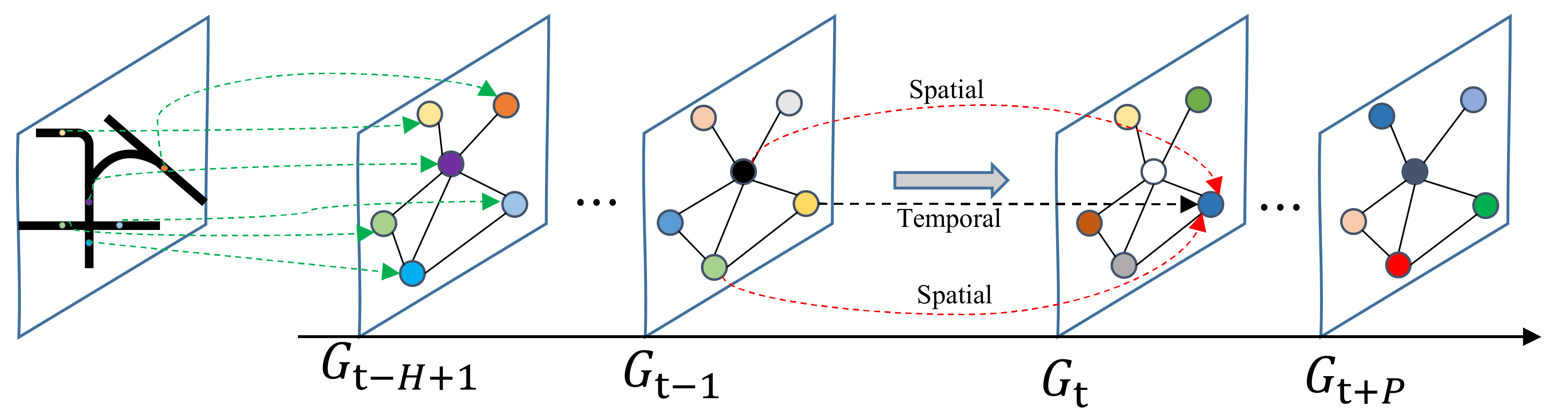
3.1.1. Spatial-Temporal Graph Prediction of Traffic Flow

In general, traffic status refers to traffic speed, flow, and density. This research chooses traffic speed to represent traffic status. We define the traffic network on a graph, the traffic flow monitoring point can be abstracted as a node in the graph, and the state of the node is the collected traffic flow information. Meanwhile, the spatial relationship between two traffic flow monitoring points can be represented by the edges of the graph. Therefore, the traffic network can be denoted as G = V , E . Give the traffic flow time series atlas { G t | t T } , where T represents the length for a graph structure with n nodes, assuming that the length of the historical observation window is H and t represents the current moment. The sequence atlas is represented as G t H + 1 , , G t , where the feature matrix corresponding to the node is V R n × i × d i = t H + 1 , t , i represents the sequence length, and d represents the node feature dimension. The spatial-temporal graph prediction of traffic flow refers to the use of historical window data to obtain a forecast atlas for a period of time in the future. Predicting the most likely traffic measurements in the next P time steps given the previous H traffic observations as
G t + 1 , G t + 2 , , G t + P arg max l o g F ( G t + 1 , , G t + P | G t H + 1 , , G t )
When converting traffic flow data into spatio-temporal graph sequence data for prediction, not only should the time series prediction of node-level feature data be considered, but also the need for the influence of the connections (edges) between nodes on the prediction should be considered spatially. Therefore, as shown in Figure 1, the spatio-temporal graph prediction of traffic flow requires the evolution of the evaluation graph at two levels of time and space, and it is obtained by the fusion of the two forecast results.

3.1.2. Graph Convolution

The graph is generally represented as G = V , E , where V represents the node set of the graph G and E is the set of edges. The most commonly used representation of the graph is the adjacency matrix: A = { a i j | v i , v j } . In order to obtain the spatial dependencies in the graph, we define the convolution operation in the frequency domain. For the traffic flow data x , the graph convolution operation G is convolved by a kernel filter F with a convolution kernel g θ , U is the eigenvector of the Laplace matrix, and the convolution operation can be expressed as:
F G x = U [ U T F L U T x = U g θ U T x
where L = I n D 1 / 2 A D 1 / 2 , D represents the degree matrix of graph G , and D i j = j A i j ,   I n R n × n is the identity matrix.
In order to simplify the calculation, the Chebyshev polynomial is usually used for approximate calculation, and the formula can be rewritten as:
F G x k = 0 K 1 θ k T k L x
where L = 2 L λ m a x I n , T k L is the Chebyshev approximation polynomial of order K . When the number of hops K = 1 , the first-order Chebyshev approximation can be obtained:
F G x θ 0 x θ 1 D 1 / 2 A D 1 / 2 x
θ 0 , θ 1 are the hyperparameters of the one-hop and two-hop nodes. Let θ = θ 0 = θ 1 , then the first-order linear expression of the graph convolution layer is expressed as:
H l = σ ( D 1 / 2 A D 1 / 2 H l 1 W l )
where H l represents the output of the lth layer, σ · is the activation function, and W represents the learnable parameter.

3.2. Methodology

3.2.1. Framework of STAWGNN

In traffic flow prediction tasks, the ability to sufficiently capture the spatial and temporal dependencies hidden in the traffic flow data is the key to modeling. This section will introduce the design of temporal feature fusion convolutional learning, spatial feature fusion convolutional learning, and spatial-temporal feature fusion convolutional blocks. In the STAWGNN model, a fusion of the graph wavelet convolution and a graph convolution applying a learnable location attention mechanism is designed for spatially dependent feature extraction of traffic flow data. Meanwhile, a fusion of temporal time attention mechanism and gated TCN is used to capture temporally dependent features. As shown in Figure 2, the overall framework designed by STAWGNN includes three parts: the input layer, spatio-temporal feature fusion extraction layer, and prediction output layer. The spatial-temporal feature extraction part consists of two spatial-temporal feature fusion convolution blocks. Each spatial-temporal convolutional block contains two temporal feature fusion convolutional layers and one spatial feature fusion convolutional layer.

3.2.2. Spatial Feature Fusion Convolutional Layer

As shown in Equation (6), the Fourier transform defines a graph convolution operation based on the spectral domain. However, this defined convolution operation can only perform feature aggregation on adjacent nodes within a certain range, which is not flexible enough. Therefore, the wavelet transform, instead of the Fourier transform, is proposed to realize the convolution theorem [28]. Compared with the Fourier transform, the graph wavelet transform aggregates local node information to characterize node features, which improves the interpretability of the method. Given the wavelet basis set ψ s , set the convolution kernel as Θ . For the input signal x R n , the graph wavelet convolution operation is defined as follows:
x G Θ = ψ s ψ s 1 x ψ s 1 Θ
where G represents the convolution operation, represents the Hadamard product, and ψ s 1 = ψ s 1 , ψ s 2 , , ψ sn is the inverse transform of ψ s .
However, in the actual traffic network, the spatial dependencies between nodes are not fixed. Therefore, a learnable location attention mechanism is designed to replace the original adjacency matrix with the new relationship matrix generated by learning. The graph convolution operation is used to capture the variable spatial dependencies between nodes. The computation of each element R   i , j in the relationship matrix learned based on the position is as Equation (7).
R i , j = e x p S c o r e p i , p j k = 1 N e x p S c o r e p i , p k
S c o r e p i , p j = p i T p j
where p i represents the potential position representation of each node, and in order to reduce the computational complexity, the relationship matrix R is sparsed with a mask:
m a s k R = R i j ,               i f   A ˜ i j > 0     0 ,             o t h e r w i s e
Perform the graph convolution operation on the newly learned relation matrix mask (R), then Formula (5) can be transformed into:
H l = σ ( D R 1 / 2 R ˜ D R 1 / 2 H l 1 W l )
where R ˜ = m a s k R + I n ,   D R is the degree matrix of R ˜ .
For the input H s l 1 after a spatial feature fusion extraction layer, the iterative formula of the output H s l is:
H s l = R e L U ( ψ s g θ ψ s 1 H l 1 W 1 l ) σ ( D R 1 / 2 R ˜ D R 1 / 2 H s l 1 W 2 l )

3.2.3. Temporal Feature Fusion Convolutional Layer

The extraction of temporal features is an unavoidable problem in traffic flow prediction tasks. The gated TCN includes two causal convolutions with H t width filter kernels. One causal convolution is followed by a sigmoid activation function to produce an output P . The other causal convolution is followed by a residual connection, which directly adds to the input to produce an output Q . The gate of sigmoid activation controls which sequences Q of the current time step are relevant for exploring dynamic correlations in the time series. Meanwhile, the sigmoid gate also contributes to the exploring of the complete input field via the multiple 1-D convolutional layers. Given the input sequence X R m × c i , where m is the length of the sequence on time axis and c i is the number of channel. The filter kernel Γ with H t width is used to produce an output with dimensions m H t + 1 × c 0 . Thus, the gated TCN can be expressed as:
Γ t X = P Q R   m H t + 1 × c 0
where is the Hadamard product, and t is the operator of gated TCN.
However, real-world traffic networks are complex. Global temporal information extraction is performed on traffic data by the temporal attention mechanism [33]. The attention function is to map a query and a set of key-value pairs to an output, where both the query and the key-value pairs are vectors. The output is a weighted sum of values, where the weight assigned to each value is determined by both the query and the corresponding key. The attention function is calculated as shown in Equation (13):
A t t e n t i o n Q , K , V = s o f t m a x ( Q K T d k V )
For input H T R T × d ,   Q = H T W Q ; K = H T W K , V = H T W V where W Q R d × d k , W V R d × d k is the projection matrix to be learned, which is shared by all nodes. Therefore, the calculation formula of the attention function can be rewritten as Formula (14):
A t t e n t i o n H T = s o f t m a x ( H i W Q H i W K T d k H T W V )
In order to jointly aggregate information from different representation subspaces, the results of multiple attention layers are integrated to improve the presentation of the model. When there are M attention layers, the multi-head attention is expressed as:
M u l t i h e a d H T = C o n c a t h e a d 1 , , h e a d M W O , h e a d M = A t t e n t i o n M H T = s o f t m a x ( ( H T W M Q ) H T W M K T d k H T W M V )
where W M Q , W M K , W M V is the projection matrix of the M th attention head, and W O is another linear output projection.
A gated TCN can obtain the temporal order correlation and is a locally relevant feature extraction method. STGAWNN can better extract temporal feature information of traffic flow by fusing a gated TCN and temporal features extracted by an attention module As shown in Figure 3 for the input H t l 1 after a temporal feature fusion extraction layer, the iterative formula for outputting H t l is:
H t l 1 = R e L U ( ( H t l Γ t ) M u l t i h e a d H t l )

3.2.4. Prediction Output Layer

After two layers of stacked spatial-temporal feature fusion convolution blocks, the input traffic flow data is mapped to a gated TCN layer for single-step prediction. Finally, the output Z of the model is linearly transformed by channel c to the final prediction result V ^ = Z w + b , where w R c is the weight vector and b is the bias. We use the L 2 loss to measure the performance of the model. The loss function of the STAGWNN model for the prediction task is Formula (17):
L V ^ , W θ = t V ^ V t H + 1 , , V t ,   W θ V t + 1 2
where W θ is the learnable parameter of the model, V t + 1 represents the true value, and V ^ · represents STAGWNN prediction result.

4. Experiment

4.1. Dataset Details

This section mainly verifies the model proposed in this paper. In the experiment, two public transportation network datasets, PEMSD7(M) [34,35] and PEMS-BAY [35,36], are used. The statistical information of these datasets is shown in Table 1.
For PEMS-BAY and PEMSD7(M), the adjacency matrix in them is calculated based on the distances between nodes. The weighted adjacency matrix W can be expressed as:
W i j = exp d i s v i , v j 2 σ 2 ,   d i s v i , v j δ       0               ,   o t h e r w i s e
where d i s   v i , v j represents the distance from node v i to node v j , and σ 2 = 10 and δ = 0.5 are thresholds to control the distribution and sparsity of matrix W i j . W i j is the value of the i th row and j th column in the weighted adjacency matrix.

4.2. Experimental Settings

All experiments were conducted on the NVIDIA A100 with 80G video memory. The size of the historical observation window is H = 12. Observations from the past hour (12 × 5 min) are used to predict the traffic conditions in the next 15, 30, and 45 min in PeMSD7(M) and 15, 30, and 60 min in PEMS-BAY. We also selected 80% of the data for training, 10% of the data for testing, and the remaining 10% of the data for validation. Table 2 gives the best hyper-parameters for training our proposed model. They are determined by trial and error.

4.3. Evaluation Indicators and Comparison Models

We adopted Mean Absolute Errors (MAE), Mean Absolute Percentage Errors (MAPE), and Root Mean Squared Errors (RMSE) to measure the prediction performance of the proposed model. The models involved in the comparison include:
  • STGCN: Spatial-temporal graph convolutional network [10], which applied ChebNet graph convolution and 1D convolution to extract spatial and temporal correlation.
  • ARIMA: Autoregressive integrated moving average model with Kalman filtering [15].
  • FC-LSTM: LSTM encoder-decoder predictor model [37] that employed a recurrent neural network with fully connected LSTM hidden units.
  • DCRNN: Diffusion convolutional recurrent neural network [22] that used diffusion graph convolutional network and RNN to learn the representation of spatial dependencies and temporal relations.
  • LSGCN: Long short-term graph convolutional network [23] that proposed a spatial gated block where a new graph attention network called cosAtt and GCN were integrated into a gated form to capture the spatial features of traffic flow data.
  • SLCNN: A spatial-temporal graph learning neural network [24] that learned the spatial features of traffic flow data through local and global pairs.
  • ASTGCN: Attention-based spatial-temporal graph convolutional network [38] that used two attention layers to capture the dynamic associations in both spatial and temporal dimensions.
  • FC-GAGA: Fully connected gated graph network [39] that performed traffic prediction without using prior knowledge of graph structure but learned spatial dependencies through gated graph modules.

4.4. Result

4.4.1. Performance Comparison

On the PEMS-BAY and PEMSD7(M) datasets, the statistics of the prediction results of the STAWGNN model and other benchmark models are shown in Table 3.
As we can see from Table 3, STAWGNN achieves the best results on both datasets of different prediction tasks. Compared with traditional models, such as HA and ARIMA, STWGNN significantly reduced the MAE, MAPE, and RMSE values. For example, the MAE values of STAWGNN for the 60-min prediction task on the PEMS-BAY dataset were 56.21% and 31.25% lower than those of ARIMA and HA, indicating that the traditional models have a limited ability to handle complex traffic flow data. DCRNN is the typical RNN-based traffic forecasting works. Limited by the capability to model long-term temporal dependencies, the forecasting accuracy is much lower than STAWGNN. LSGCN provides better results than STGCN models. This is because the adaptive graph matrix learned by the graph attention-based network can automatically discover the invisible graph structure from the data. Compared to the LSGCN model, the SLCNN model performs better on both datasets across different prediction tasks, except for the 15-min. Among deep learning models, STAWGNN still performs the best. For example, for the 60-min prediction on the PEMS-BAY dataset, the MAPE and RMSE values are reduced by 4.24% and 5.00%, respectively. Meanwhile, compared to other graph-based works, STAWGNN achieves superior performance, especially on the RMSE and MAPE metrics, for all datasets. This is because the graph wavelets layer significantly improves the capability to capture local changing spatial heterogeneity.

4.4.2. Performance Analysis of Graph Wavelet Neural Network

In the spectral convolutional neural network (Spectral CNN) [40], feature aggregation needs to be performed on a certain range of neighboring nodes by specifying the number of hops, which makes the domain of the central node strictly limited by a circle of specified radius. Therefore, Spectral CNN the limited local feature extraction capability. In order to solve the shortcomings of Spectral CNN, the STAWGNN model uses the graph wavelet transform to capture the local spatial topology of the road network. The distribution of the zero values of the graph wavelet matrix in the two datasets is shown in Table 4.
It can be seen that the percentage of non-zero elements in each graph wavelet transform matrix ψ s 1 is 21.7% and 19.2%, respectively. The Fourier transform matrix U T has 99.71% and 98.32% non-zero elements, respectively. This result indicates that the graph wavelet matrix is sparser than the Fourier transform matrix in both datasets. In addition, we also analyze the performance of Spectral CNN with GWNN on two datasets. Figure 4 shows the comparison between the STAWGNN and Spectral CNN-based model on the next 60-min prediction task. It can be seen that with the increase in the prediction time, the changes in MAE and RMSE values show an upward trend, which shows that the performance of model prediction will decrease with an increase in the prediction step size. For the prediction tasks from 5 to 60 min, the change curves of MAE and RMSE values of the STAGWNN model based on graph wavelet transform are located above the Spectral CNN-based model. This result indicates that the STAWGNN model has better performance than the Spectral CNN model.
In the graph wavelet convolution layer, the size of the information diffusion neighborhood of each node is controlled by a hyper-parameter. Since the state of the node neighborhood information affects the changing trend of the central node, the appropriate neighborhood size is conducive to improving the model’s performance. Therefore, in order to explore the effect of the scale factor on the performance of STAGWNN. The scale factors of the PEMS-BAY and PEMSD7(M) datasets are compared. Figure 5 shows the MAE and RMSE on the two datasets in the 15-min prediction task. It can be seen that when s = 0.05, the error is at its minimum.

4.4.3. Influence of Attention Mechanism

To verify the effectiveness of the attention mechanism in STAGWNN, comparative experiments were also designed on the two datasets. The model names without the different components are as follows:
  • w/o ST-Att: STAWGNN without spatial and temporal attention mechanisms.
  • w/o S-Att: STAWGNN without spatial attention mechanism. Only graph wavelet networks are used in spatial feature extraction to capture the local spatial features hidden in the traffic flow data.
  • w/o T-Att: STAWGNN without temporal attention mechanism. Gated TCNs are only used to capture local temporal features in traffic flow data.
The experimental results on the two datasets for different prediction tasks are shown in Figure 6 and Figure 7.
From Figure 6 and Figure 7, we can see that the prediction performance of the proposed STAWGNN model has the best prediction performance on the two different dataset prediction tasks. This is mainly because the STAWGNN model not only captures the inherent spatial relationships of the road network but also learns the time-varying spatial dependencies of each node through the learnable attention mechanism of the location. After removing the attention mechanism, with the forecast time increases, the performance of our model gradually deteriorates more significantly. We conjecture that the reason is that the long-term spatial-temporal dependencies have changed significantly. On the PEMS-BAY dataset, the heat map of the adjacency matrix obtained for the top 50 nodes under different methods is shown in Figure 8. In it, the lighter blue color indicates that the node is more followed, while the darker blue color indicates that the node is less followed. Compared with the adjacency matrix calculated from the distances between nodes in the real road network in Figure 8a, the adjacency matrix derived from the location-based learnable attention mechanism in Figure 8b can extract additional spatial feature information of the road nodes from a global perspective.

4.4.4. Traffic Flow Data Analysis

The actual value and the predicted value obtained by the STAWGNN model of the traffic flow data in one day are compared and analyzed. Since the time interval of data collection is 5 min, the amount of data collected in one day is 288. In order to better evaluate the performance of our model in a practical application, we visualize the predicted traffic flow of a certain node on the two datasets shown in Figure 9. It can be seen, compared with SLGCN and FC-GAGA, that STAGWNN can better fit the real value. Meanwhile, the mutation of a time period can also be well fitted, e.g., t 100 , 150 on the PEMS-BAY dataset, which indicates that the STAWGNN model can better capture the sudden changes in the signal and detect the peaks in the signal. In addition, STAWGNN can capture continuous changes within long steps, e.g., t 150 , 200 on the PEMSD7(M) dataset. This fact implies that dynamical spatial dependencies and long-range temporal dependencies captured by STAWGNN benefit traffic flow forecasting, especially long-term prediction.

5. Conclusions

This paper proposed an attention and wavelet-based spatial-temporal graph neural network for traffic flow and speed prediction. The model used a graph wavelet neural network and location-learnable attention mechanism to extract local and global spatial correlations in traffic flow data. For time series information extraction, we stacked a gated TCN with temporal attention mechanisms to extract local and global dependencies of time series information. Experiments showed that this method could better aggregate traffic flow information from adjacent roads and improve the prediction accuracy. However, the lack of seasonality and periodicity analysis in modeling traffic flow data is a shortcoming of this study. Finally, how to further improve the robustness of the model and use the model to solve real traffic congestion problems will be our future work.

Author Contributions

G.M.: methodology conceptualization and design of the experimental framework; S.Z.: conceived and designed the experiments, analyzed the data, and wrote the paper; G.M., S.Z. and S.X.: formal analysis; S.Z.: writing—original draft preparation; G.M. and S.X.: writing—review and editing. All authors have read and agreed to the published version of the manuscript.

Funding

This work was supported by grants from National Natural Science Foundation of China (61773415) and National Key Research and Development Project of China (2019YFD0900805).

Institutional Review Board Statement

This study did not involve humans or animals.

Informed Consent Statement

This study did not involve humans.

Data Availability Statement

Not applicable.

Conflicts of Interest

The authors declare no conflict of interest. The funders had no role in the design of the study.

References

  1. Yuen, M.; Ng, S.C.; Leung, M.F. A competitive mechanism multi-objective particle swarm optimization algorithm and its application to signalized traffic problem. Cybern. Syst. 2020, 52, 73–104. [Google Scholar] [CrossRef]
  2. Huang, K.W.; Chen, G.W.; Huang, Z.H.; Lee, S.H. Anomaly Detection in Airport based on Generative Adversarial Network for Intelligent Transportation System. In Proceedings of the 2022 IEEE International Conference on Consumer Electronics-Taiwan, Taiwan, China, 6–8 July 2022; pp. 311–312. [Google Scholar]
  3. Yang, S.; Lu, H.; Li, J. Multifeature Fusion-Based Object Detection for Intelligent Transportation Systems. IEEE Trans. Intell. Transp. Syst. 2022, 1–8. [Google Scholar] [CrossRef]
  4. Nagy, A.M.; Simon, V. Survey on traffic prediction in smart cities. Pervasive Mob. Comput. 2018, 50, 148–163. [Google Scholar] [CrossRef]
  5. Han, S.; Kim, J. Video scene change detection using convolution neural network. In Proceedings of the 2017 International Conference on Information Technology, Singapore, 27–29 December 2017; pp. 116–119. [Google Scholar]
  6. Quamer, W.; Jain, P.K.; Rai, A.; Saravanan, V.; Pamula, R.; Kumar, C. SACNN: Self-attentive convolutional neural network model for natural language inference. Trans. Asian Low-Resour. Lang. Inf. Processing 2021, 20, 50. [Google Scholar] [CrossRef]
  7. Caliwag, E.M.F.; Caliwag, A.; Baek, B.K.; Jo, Y.; Chung, H.; Lim, W. Distance Estimation in Thermal Cameras Using Multi-Task Cascaded Convolutional Neural Network. IEEE Sens. J. 2021, 21, 18519–18525. [Google Scholar] [CrossRef]
  8. Lim, B.; Zohren, S. Time-series forecasting with deep learning: A survey. Philos. Trans. R. Soc. A 2021, 379, 20200209. [Google Scholar] [CrossRef] [PubMed]
  9. Zhao, L.; Song, Y.; Zhang, C.; Liu, Y.; Wang, P.; Lin, T.; Deng, M.; Li, H. T-gcn: A temporal graph convolutional network for traffic prediction. IEEE Trans. Intell. Transp. Syst. 2019, 21, 3848–3858. [Google Scholar] [CrossRef]
  10. Yu, B.; Yin, H.; Zhu, Z. Spatio-Temporal Graph Convolutional Networks: A Deep Learning Framework for Traffic Forecasting. In Proceedings of the IJCAI, Stockholm, Sweden, 13–19 July 2018; pp. 3634–3640. [Google Scholar]
  11. Jiang, W.; Luo, J. Graph neural network for traffic forecasting: A survey. Expert Syst. Appl. 2022, 207, 117921. [Google Scholar] [CrossRef]
  12. Wu, Z.; Pan, S.; Long, G.; Jiang, J.; Chang, X.; Zhang, C. Connecting the dots: Multivariate time series forecasting with graph neural networks. In Proceedings of the KDD ‘20: The 26th ACM SIGKDD Conference on Knowledge Discovery and Data Mining, Virtual, San Diego, CA, USA, 6–10 July 2020; pp. 753–763. [Google Scholar]
  13. Chen, Y.; Wu, L.; Zaki, M. Iterative deep graph learning for graph neural networks: Better and robust node embeddings. Adv. Neural Inf. Processing Syst. 2020, 33, 19314–19326. [Google Scholar]
  14. Wu, Z.; Pan, S.; Long, G.; Jiang, J.; Zhang, C. Graph wavenet for deep spatial-temporal graph modeling. In Proceedings of the IJCAI, Macao, China, 10–16 August 2019. [Google Scholar]
  15. Kumar, S.V.; Vanajakshi, L. Short-term traffic flow prediction using seasonal ARIMA model with limited input data. Eur. Transp. Res. Rev. 2015, 7, 21. [Google Scholar] [CrossRef]
  16. Cai, L.; Zhang, Z.; Yang, J.; Yu, Y.; Qin, J. A noise-immune Kalman filter for short-term traffic flow forecasting. Phys. A Stat. Mech. Its Appl. 2019, 536, 122601. [Google Scholar] [CrossRef]
  17. Smola, A.J.; Schölkopf, B. A tutorial on support vector regression. Stat. Comput. 2004, 14, 199–222. [Google Scholar] [CrossRef]
  18. Keller J, M.; Gray M, R.; Givens J, A. A fuzzy k-nearest neighbor algorithm. IEEE Trans. Syst. Man Cybern. 1985, 4, 580–585. [Google Scholar] [CrossRef]
  19. Yu, R.; Li, Y.; Shahabi, C.; Demiryurek, U.; Liu, Y. Deep learning: A generic approach for extreme condition traffic forecasting. In Proceedings of the 2017 SIAM International Conference on Data Mining, Houston, TX, USA, 27–29 April 2017; pp. 777–785. [Google Scholar]
  20. Zhang, J.; Zheng, Y.; Qi, D. Deep spatio-temporal residual networks for citywide crowd flows prediction. In Proceedings of the Thirty-First AAAI Conference on Artificial Intelligence, San Francisco, CA, USA, 4–9 February 2017. [Google Scholar]
  21. Zhang, J.; Zheng, Y.; Qi, D.; Li, R.; Yi, X. DNN-based prediction model for spatio-temporal data. In Proceedings of the SIGSPATIAL’16: 24th ACM SIGSPATIAL International Conference on Advances in Geographic Information Systems, Burlingame, CA, USA, 31 October–3 November 2016; pp. 1–4. [Google Scholar]
  22. Li, Y.; Yu, R.; Shahabi, C.; Liu, Y. Diffusion Convolutional Recurrent Neural Network: Data-Driven Traffic Forecasting. In Proceedings of the International Conference on Learning Representations, Vancouver, BC, Canada, 30 April–3 May 2018. [Google Scholar]
  23. Huang, R.; Huang, C.; Liu, Y.; Dai, G.; Kong, W. LSGCN: Long Short-Term Traffic Prediction with Graph Convolutional Networks. In Proceedings of the Twenty-Ninth International Joint Conference on Artificial Intelligence and Seventeenth Pacific Rim International Conference on Artificial Intelligence, Yokohama, Japan, 7–15 January 2021; pp. 2355–2361. [Google Scholar]
  24. Zhang, Q.; Chang, J.; Meng, G.; Xiang, S.; Pan, C. Spatio-temporal graph structure learning for traffic forecasting. In Proceedings of the AAAI Conference on Artificial Intelligence, New York, NY, USA, 7–12 February 2020; pp. 1177–1185. [Google Scholar]
  25. Xu, B.; Shen, H.; Cao, Q.; Qiu, Y.; Cheng, X. Graph wavelet neural network. In Proceedings of the IJCAI, Macau, China, 10–16 August 2019. [Google Scholar]
  26. Cui, Z.; Ke, R.; Pu, Z.; Ma, X.; Wang, Y. Learning traffic as a graph: A gated graph wavelet recurrent neural network for network-scale traffic prediction. Transp. Res. Part C Emerg. Technol. 2020, 115, 102620. [Google Scholar] [CrossRef]
  27. Zhang, M.; Chen, Y. Link prediction based on graph neural networks. In Proceedings of the Advances in Neural Information Processing Systems, Montreal, QC, Canada, 3–8 December 2018; pp. 5165–5175. [Google Scholar]
  28. Kipf, T.N.; Welling, M. Semi-supervised classification with graph convolutional networks. In Proceedings of the International Conference on Learning Representations, Toulon, France, 24–26 April 2017. [Google Scholar]
  29. Zhang, C.; Song, D.; Huang, C.; Swami, A.; Chawla, N.V. Heterogeneous graph neural network. In Proceedings of the 25th ACM SIGKDD International Conference on Knowledge Discovery & Data Mining, Anchorage, AK, USA, 4–8 August 2019; pp. 793–803. [Google Scholar]
  30. Xie, Z.; Chen, J.; Peng, B. Point clouds learning with attention-based graph convolution networks. Neurocomputing 2020, 402, 245–255. [Google Scholar] [CrossRef]
  31. Liu, Z.; Chen, C.; Li, L.; Zhou, J.; Li, X.; Song, L.; Qi, Y. Geniepath: Graph neural networks with adaptive receptive paths. In Proceedings of the AAAI Conference on Artificial Intelligence, Honolulu, HI, USA, 27 January–1 February 2019; pp. 4424–4431. [Google Scholar]
  32. Li, R.; Wang, S.; Zhu, F.; Huang, J. Adaptive graph convolutional neural networks. In Proceedings of the Thirty-Second AAAI Conference on Artificial Intelligence, New Orleans, LO, USA, 2–7 February 2018. [Google Scholar]
  33. Vaswani, A.; Shazeer, N.; Parmar, N.; Uszkoreit, J.; Jones, L.; Gomez, A.N.; Polosukhin, I. Attention is all you need. Adv. Neural Inf. Processing Syst. 2017, 30. [Google Scholar] [CrossRef]
  34. Roy, A.; Roy, K.K.; Ali, A.A.; Amin, M.A.; Rahman, A.M. Unified spatio-temporal modeling for traffic forecasting using graph neural network. In Proceedings of the 2021 International Joint Conference on Neural Networks (IJCNN), Shenzhen, China, 18–22 July 2021; pp. 1–8. [Google Scholar]
  35. Li, M.; Zhu, Z. Spatial-temporal fusion graph neural networks for traffic flow forecasting. In Proceedings of the AAAI Conference on Artificial Intelligence, Virtual, CA, USA, 2–9 February 2021; Volume 35, pp. 4189–4196. [Google Scholar]
  36. Li, F.; Feng, J.; Yan, H.; Jin, G.; Yang, F.; Sun, F.; Li, Y. Dynamic graph convolutional recurrent network for traffic prediction: Benchmark and solution. ACM Trans. Knowl. Discov. Data (TKDD) 2021. [Google Scholar] [CrossRef]
  37. Sutskever, I.; Vinyals, O.; Le, Q.V. Sequence to sequence learning with neural networks. In Proceedings of the Advances in Neural Information Processing Systems, Montreal, QC, Canada, 3–8 December 2014; Volume 27. [Google Scholar]
  38. Guo, S.; Lin, Y.; Feng, N.; Song, C.; Wan, H. Attention based spatial-temporal graph convolutional networks for traffic flow forecasting. In Proceedings of the AAAI Conference on Artificial Intelligence, Honolulu, HI, USA, 27–28 January 2019; Volume 33, pp. 922–929. [Google Scholar]
  39. Oreshkin, B.N.; Amini, A.; Coyle, L.; Coates, M. FC-GAGA: Fully connected gated graph architecture for spatio-temporal traffic forecasting. In Proceedings of the AAAI Conference on Artificial Intelligence, Virtual, CA, USA, 2–9 February 2021; pp. 9233–9241. [Google Scholar]
  40. Bruna, J.; Zaremba, W.; Szlam, A.; LeCun, Y. Spectral networks and locally connected networks on graphs. In Proceedings of the International Conference on Learning Representations, Banff, AL, Canada, 14–16 April 2014. [Google Scholar]
Figure 1. Schematic diagram of the evolution of the spatio-temporal graph prediction of traffic flow.
Mathematics 10 03507 g001
Figure 2. Overall Architecture of the STAGWNN model.
Mathematics 10 03507 g002
Figure 3. Temporal feature fusion layer. σ represents the sigmoid activation function and ⊗ represents the element-wise Hadamard product between two branches. P and Q are the outputs of Casual Conv.
Mathematics 10 03507 g003
Figure 4. Performance comparison between STWGNN and Spectral CNN for the next 60 min prediction task. (a,b) are the variation curves of MAE and RMSE on the PEMS-BSY dataset, respectively; (c,d) are the variation curves of MAE and RMSE on the PEMSD7(M) dataset, respectively.
Mathematics 10 03507 g004
Figure 5. Curves of MAE and RMSE of PEMS-BAY(a) and PEMSD7(M) (b) datasets as a function of scale factor S.
Mathematics 10 03507 g005
Figure 6. Component analysis of STAWGNN on the PEMSD-BAY dataset.
Mathematics 10 03507 g006
Figure 7. Component analysis of STAWGNN on the PEMSD7(M) dataset.
Mathematics 10 03507 g007
Figure 8. Adjacency matrix for the top 50 nodes of the PEMS-BAY dataset. (a) is the visualization of the adjacency matrix calculated from the distances between nodes in the real road network; (b) is the visualization of adjacency matrix derived from the location-based learnable attention mechanism.
Mathematics 10 03507 g008
Figure 9. Comparison of predicted and true values of the speed of the two datasets.
Mathematics 10 03507 g009
Table 1. Dataset Statistics.
DatasetNodeEdge NumberTime StepsTime IntervalLongUnit
PEMS-BAY325236952,1165 min12km/h
PEMSD7(M)22883212,6725 min12km/h
Table 2. Optimal hyper-parameter settings for training our proposed model.
DatasetBatch SizeEpochsLearning RateDropout RateSOptimizer
PEMS-BAY321000.00010.50.05Adam
PEMSD7(M)321000.00010.50.05Adam
Table 3. The prediction performance of different models on the two datasets.
PMDS-BAY15 min30 min60 min
MAEMAPERMSEMAEMAPERMSEMAEMAPERMSE
HA2.886.80%5.592.886.80%5.592.886.80%5.59
ARIMA1.623.50%3.302.335.40%4.763.388.30%6.50
FC-LSTM2.054.80%4.192.205.20%4.552.375.70%4.96
DCRNN1.382.90%2.951.743.90%3.972.074.90%4.74
STGCN1.372.95%2.981.854.22%4.342.495.81%5.70
ASTGCN1.523.22%3.132.014.48%4.272.616.00%5.42
LSGCN1.422.87%2.712.024.13%4.153.136.11%6.16
SLCNN1.443.00%2.901.73%4.10%3.812.034.80%4.53
FC-GAGA1.342.82%2.821.663.71%3.751.934.48%4.40
STAWGNN1.262.53%2.571.663.43%3.531.984.29%4.18
PMDS7(M)15 min30 min45 min
MAEMAPERMSEMAEMAPERMSEMAEMAPERMSE
HA4.0110.61%7.204.0110.61%7.204.0110.61%7.20
ARIMA5.5512.92%9.005.8613.94%9.136.6816.78%9.68
FC-LSTM3.578.60%6.203.929.55%7.034.1610.10%7.51
DCRNN2.375.54%4.213.318.06%5.964.019.99%7.13
STGCN2.255.26%4.043.037.33%5.703.578.69%6.77
ASTGCN2.857.25%5.153.358.67%6.123.9610.56%7.20
LSGCN2.225.14%3.982.967.18%5.473.438.51%6.39
SLCNN2.225.21%4.072.887.17%5.503.278.20%6.28
FC-GAGA2.185.29%4.152.807.06%5.583.318.47%6.66
STAWGNN2.185.07%3.952.886.95%5.283.317.99%6.03
The best results are in bold.
Table 4. Graph wavelet matrix sparsity statistics.
DatasetTotal Number of ElementsThe Number of Non-Zero ValueProportion of Non-Zero Valued
PEMS-BAY104,32922,70721.7%
PEMSD7(M)50,350966719.2%
Publisher’s Note: MDPI stays neutral with regard to jurisdictional claims in published maps and institutional affiliations.

