Two Novel Non-Uniform Quantizers with Application in Post-Training Quantization

Abstract

With increased network downsizing and cost minimization in deployment of neural network (NN) models, the utilization of edge computing takes a significant place in modern artificial intelligence today. To bridge the memory constraints of less-capable edge systems, a plethora of quantizer models and quantization techniques are proposed for NN compression with the goal of enabling the fitting of the quantized NN (QNN) on the edge device and guaranteeing a high extent of accuracy preservation. NN compression by means of post-training quantization has attracted a lot of research attention, where the efficiency of uniform quantizers (UQs) has been promoted and heavily exploited. In this paper, we propose two novel non-uniform quantizers (NUQs) that prudently utilize one of the two properties of the simplest UQ. Although having the same quantization rule for specifying the support region, both NUQs have a different starting setting in terms of cell width, compared to a standard UQ. The first quantizer, named the simplest power-of-two quantizer (SPTQ), defines the width of cells that are multiplied by the power of two. As it is the case in the simplest UQ design, the representation levels of SPTQ are midpoints of the quantization cells. The second quantizer, named the modified SPTQ (MSPTQ), is a more competitive quantizer model, representing an enhanced version of SPTQ in which the quantizer decision thresholds are centered between the nearest representation levels, similar to the UQ design. These properties make the novel NUQs relatively simple. Unlike UQ, the quantization cells of MSPTQ are not of equal widths and the representation levels are not midpoints of the quantization cells. In this paper, we describe the design procedure of SPTQ and MSPTQ and we perform their optimization for the assumed Laplacian source. Afterwards, we perform post-training quantization by implementing SPTQ and MSPTQ, study the viability of QNN accuracy and show the implementation benefits over the case where UQ of an equal number of quantization cells is utilized in QNN for the same classification task. We believe that both NUQs are particularly substantial for memory-constrained environments, where simple and acceptably accurate solutions are of crucial importance.

1. Introduction

The Internet of Things (IoTs) facilitates automatization and simplification of many daily tasks in the commercial, industrial and infrastructure fields. As the number of connected IoT devices constantly grows, the IoTs seem to become an unavoidable part of our everyday life. Due to the rapid proliferation of IoTs, as predicted by [1], the volume of data generated by IoTs is increasing ceaselessly. Therefore, an efficient utilization of cloud computing resources is of great importance and requires a prudent strategy for the bandwidth usage, energy consumption and computational and memory costs [2]. Many applications for the interconnected devices in the IoT environment require or prefer fast, real-time communications with the cloud. To avoid delays in interactions with the cloud servers, the idea of edge computing has been increasingly used [3]. Although edge computing devices are less powerful than the cloud servers and are subject to many constraints, edge computing allows storing data and executing applications on the edge, directly connected with IoT devices. Further, an intersection of artificial intelligence (AI) and edge computing has introduced the concept that brings AI to the edge [4]. Achieving efficient edge computing with an acceptable or high accuracy of neural networks (NNs) requires the utilization of different techniques, such as pruning, neural network quantization, knowledge distillation, manual design of efficient architecture, neural network architecture search, etc., as profoundly discussed in [5,6]. Although these techniques can be as essential as complex, they require comprehensive rethinking of NN design to enable fitting of NNs to the memory of the edge device at first place.

One of the vulnerabilities of brining AI solutions to the edge can be reflected in the accuracy degradation of built-in NNs. Driven by the need for compression of NN parameters, which is especially beneficial for the memory-efficient deployment of NN on resource-constrained devices, numerous papers have already confirmed abundant opportunities for NN parameter compression by means of quantization [7,8,9,10,11,12,13,14]. The quantization process introduces a quantization error [15], which accumulation can cause an incorrect output of the quantized NN (QNN), thus degrading the accuracy, compared to the NN. As quantization error is the quality indicator of every quantizer, it is of particular interest to examine its relation to the QNN accuracy. Not so obvious relations between NN and its quantized counterpart, QNN, can be examined on the simple classification task [14,16,17,18,19], by analyzing the classification accuracy and achieved experimental and theoretical signal to quantization noise ratio (SQNR) values. To the best of our knowledge, SQNR is not an unambiguous fidelity measure of the QNN model, since the highest SQNR does not necessarily guarantee the highest accuracy of QNN [14]. However, in traditional quantization, it is of utmost importance for a quantizer design to determine a set of parameters that provide the maximum of SQNR [20,21,22,23]. Therefore, in this paper, we do not only propose two novel non-uniform quantizers (NUQs), but we also perform their optimization to achieve minimal distortion, i.e., maximal SQNR. In addition, we apply these NUQs in post-training quantization and examine the accuracy preservation for the same classification task, as in [14,18,19]. To make our analysis even wider, we analyze experimental and theoretical SQNR values and the accuracy of the QNN (for MLP and CNN) for a few significant cases of designing both implemented NUQs and for two datasets.

2. Related Work and Motivation

To achieve both simplicity and efficiency, most of the recent research in the field of NN compression have focused on post-training quantization, rather than on quantization-aware training [5,6]. The core idea of post-training quantization reflects on the compression of NN model weights after training the NN. Since the original NN parameters are typically stored in FP32 format, quantization can bring unique opportunities in implementing compressed NN models, as long as the quantized NN parameters have relatively close values as the original ones [19]. Despite the high difference between the QNN model and the original one (NN before quantization), it has been shown in [19] that the accuracy of the neural network can be slightly degraded after the quantization is performed. Admittedly, the accuracy gap between the full-precision NN and QNN can be still very large in some cases, with the apparent space for improvements, especially for the extremely low-bit QNNs [6,10,17,24,25].

Generally, in low-bit quantization, a very small number of bits per sample is used to represent the data being quantized (less than or equal to 3 bit/sample) [20]. Relying on plenty of quantization models from the signal processing area, quantization has proved to be an efficient technique that can perform signal compression according to some of the underlying criteria [15,21,22,23]. Many efforts in classical compression by means of quantization have been made towards the minimization of an inevitable quantization error for a given bit-rate. The main goal in compression is actually to minimize the bit-rate. However, in general, the smaller the bit-rate, the lower the storage cost and computation requirements, but the higher the quantization error [20]. These conflicting requirements mean quantization is a very intriguing area of research, specifically the choice of the quantization model itself and specification of its key parameters (the support region, quantization steps, bit-rate, decision and representation levels [15,20,21,22,23]) affect the amount of the total quantization error, that is, the total distortion. Following the main aspect of signal coding and compression, which is the bit-rate shrinkage, we can expect that for non-uniform sources, such as the Laplacian one assumed in this paper, non-uniform quantization allows better utilization of the available bit rate. Additional constraints, especially for low-bit conditions, include non-uniform quantizers that should be well suited to the lower design complexity and implementation requirements.

Unlike in our previous works, where we addressed low-bit uniform quantizer (UQ), two-bit and three-bit UQ [18,19], respectively, in this paper, we propose two novel non-uniform two-bit quantization models and we analyze QNN performance for the same classification task as the one reported in [18,19]. Our goal is to improve both the SQNR and the accuracy of the QNN model, compared to two-bit UQ from [18]. In this research, we show that this goal is achievable by utilizing the novel NUQs that will be specified in detail in the following. Let us highlight that to provide a fair comparison with the results from [18,19], in this paper, the identical multilayer perceptron (MLP) architecture is assumed, while the identical weights (stored in FP32 format) are non-uniformly quantized according to completely novel quantization rules by also using only two bits per sample. Our motivation to address the two-bit NUQs stems from the fact that non-uniform quantizers are more convenient for non-uniform distributions, as the Laplacian pdf. Having in mind that the weights distribution can closely fit some of well-known probability density functions (pdfs), as the Laplacian pdf is [7,8,12]; in this paper, as in [18,19], we assume the Laplacian-like distribution for experimental weights distribution and the Laplacian pdf for the theoretical distribution of weights, for estimating the performance of our two novel non-uniform quantizers in question. The main reason why we chose to utilize two-bit quantizers lies in an already confirmed premise for the two-bit UQ [18], that quantizer parameterization has been shown to be crucial not only for the performance of the quantizer alone but also for the QNN model accuracy, due to only four representations being available. In brief, the performance gain over UQ is relatively easily achieved by means of high-bit non-uniform quantization [22], where this is not a case with low-bit non-uniform quantization due to the small number of representations available. This makes low-bit non-uniform quantization, as the one addressed in this paper, more intriguing to research.

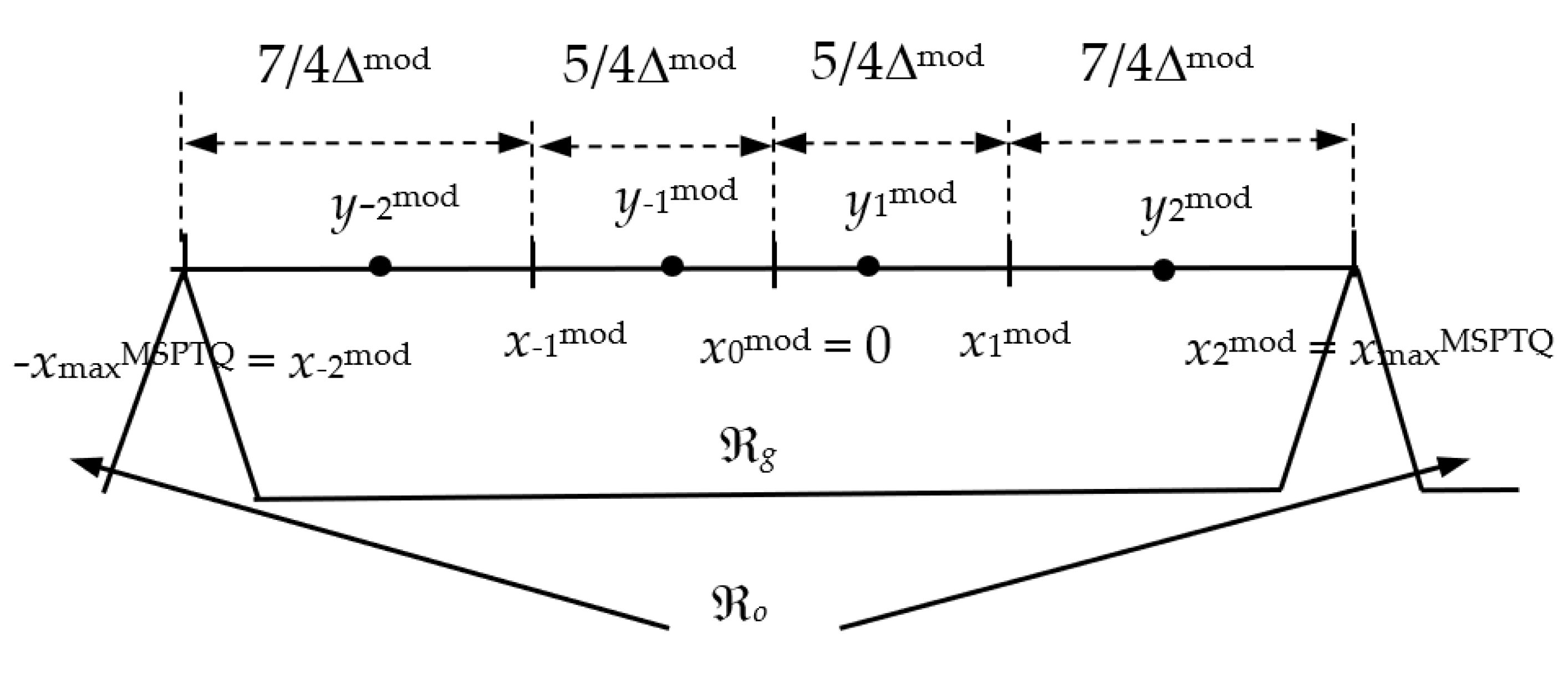
To alleviate the shortage of UQ applied to non-uniform distributions, reflected in uniform quantization of all weight values with most of them aggregated near the mean, in this paper, we specify the novel quantization rules for two-bit NUQs. More precisely, in our first novel NUQ, the quantization cell that lies inwardly closest to the mean, is of width Δ, while the width of subsequent cell, that lies in the rest of the support region is 2Δ, so that the quantizer’s support region ranges [−3Δ, 3Δ]. Hereinafter we utilize notations simplest power-of-two quantizer (SPTQ) for the first quantizer and modified simplest power-of-two quantizer (MSPTQ), as it is the modified and enhanced SPTQ version. Both aforementioned quantization models, SPTQ and MSPTQ, follow the same predefined rule for defining the support region ranging [−3Δ, 3Δ] or [−3Δ^mod, 3Δ^mod], respectively, while differing in the way of specifying the decision and representation levels of the quantizer. In SPTQ design, the representation levels are the midpoints of the quantization cells, as it is the case in the simplest UQ design, while its quantization cells are not of equal widths, as is the case with UQ. In MSPTQ design, the quantizer decision thresholds are centered between the nearest representation levels, similar to the UQ design. However, unlike UQ, the quantization cells of MSPTQ are not of equal widths and the representation levels are not midpoints of the quantization cells. More details about SPTQ and MSPTQ models will be provided in the following sections. Intending to determine the parameters of the novel quantizers more favorably and as precise as possible, we also provide a studious analysis and the description of the optimization procedure of two-bit SPTQ and MSPTQ. Specifically, we describe their design for the assumed Laplacian source and perform their optimization in an iterative manner, as well as by performing numerical optimization procedure. Afterwards, we perform post-training quantization with the implementation of SPTQ and MSPTQ, study the viability of QNN accuracy and present the benefits in the case where two-bit UQ from [18] is utilized for the same classification task. We believe that both NUQs are particularly substantial for memory-constrained devices, where simple and acceptably accurate solutions are one of the key requirements.

The rest of this paper is organized as follows: Section 3 and Section 4 describe the design of symmetrical SPTQ and MSPTQ for the Laplacian source. Section 5 briefly describes the application of novel NUQs in post-training quantization. Section 6 provides the discussion on the numerical results for two novel NUQs specified in Section 3 and Section 4. Finally, Section 7 summarizes the paper contributions and concludes our research results.

3. Symmetric SPTQ Design for the Laplacian Source

Quantization is ubiquitous in signal processing, and it specifies a mapping of continuous data to a discrete set of N quantization or representation levels [20]. The primary goal of quantization is to minimize the distortion, i.e., the deviation of the quantized signal (Q_N(X)), compared to the original (X), for a given N and bit-rate R, where R = log₂N [20]

$$D=E\left[{\left(X-Q_N\left(X\right)\right)}^2\right]$$

(1)

Specifically, the choice of the quantizer model itself and its parameterization affect the total amount of the quantization error. Therefore, in the following, we describe two novel NUQs and we specify the expressions to quantify their quantization error.

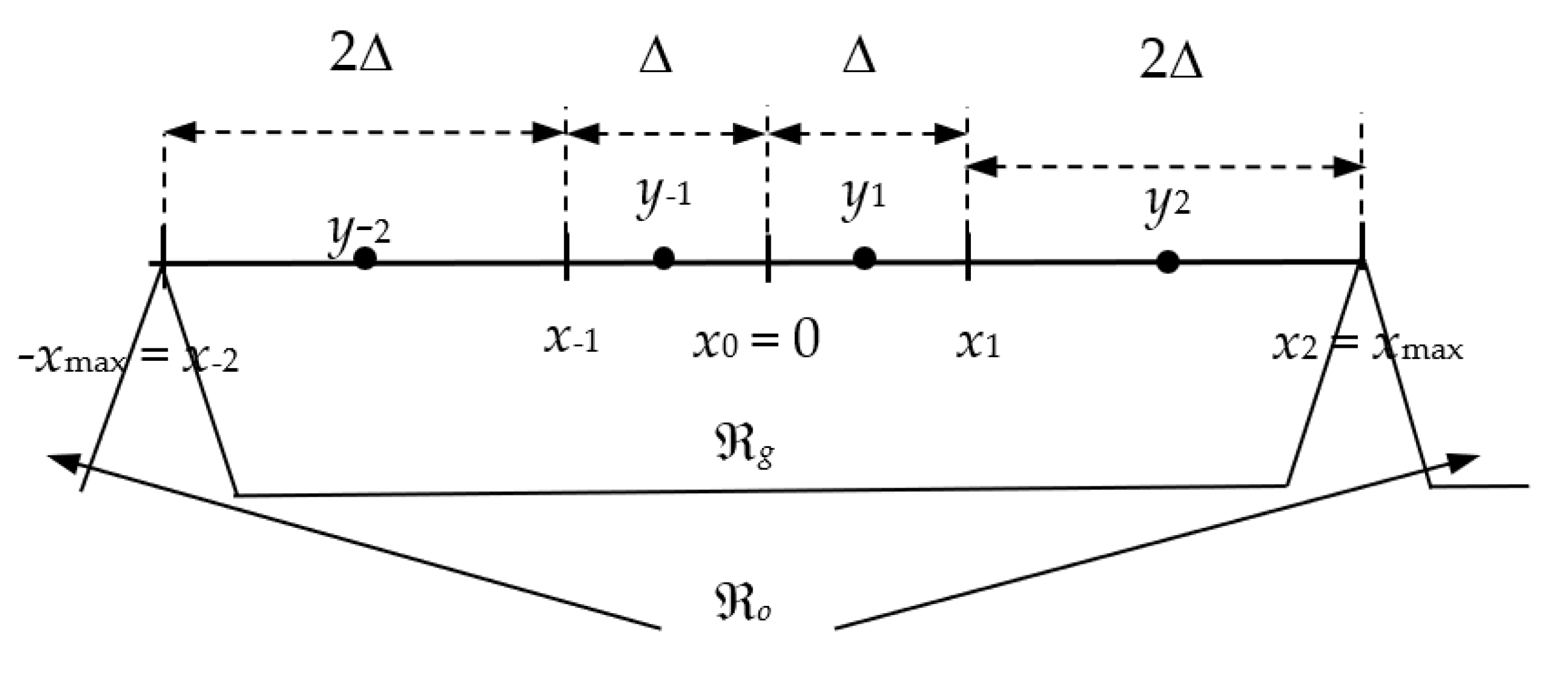
Let us first specify the key parameter of an N-level symmetrical quantizer Q_N. By the quantization procedure, an input signal amplitude range is divided into a granular region ℜ_g and an overload region ℜ_o (see Figure 1 for SPTQ). For any symmetric quantizer, as those we design here, these regions are separated by the support region thresholds denoted by −x_max and x_max, respectively [20]. The granular region ℜ_g

$${\Re }_g={\displaystyle \underset{i=-N/2}{\overset{-1}{\cup }}{\Re }_i}\cup {\displaystyle \underset{i=1}{\overset{N/2}{\cup }}{\Re }_i}=\hspace{0.33em}\left[-x_{\max },x_{\max }\right]\hspace{0.33em}\hspace{0.33em}\hspace{0.33em}$$

(2)

consists of N nonoverlapped limited in width quantization cells, where the i^th cell is:

$${\Re }_i=\left\{x\right|x \in [-x_{\max },x_{\max }],Q_N\left(x\right)=y_i\},{\Re }_i\cap {\Re }_j=\varnothing ,i\ne j$$

(3)

while y_i denotes the ith representation level and ${\left\{{\Re }_i \right\}}_{i=-N/2}^{-1}$ and ${\left\{{\Re }_i \right\}}_{i=1}^{N/2}$ denote the granular cells from the negative and positive amplitude regions, which are symmetrically placed around the zero mean. In symmetric quantization, the quantizer’s main parameter sets are halved, since only the positive or the absolute values of the quantizer’s parameters should be determined and stored. The symmetry also holds for the overload cells, that is, for a pair of quantization cells unlimited in width in the overload region, ℜ_o, defined as

$${\Re }_0=\left\{x\right|x\notin [-x_{\max },x_{\max }],Q_N\left(x\right)=y_{N/2},x>0\vee Q_N\left(x\right)=y_{-N/2},x<0\}$$

(4)

If the cells are of nonequal width, then the quantizer is non-uniform [20], as is the case with the two-bit SPTQ we address here.

Let us denote with Δ the step size of the cells of our symmetrical two-bit SPTQ that are the closest ones to the mean (see Figure 1). We further assume that the decision thresholds are not equidistant, as it is the case in UQ design. Specifically, suppose that the width of the adjacent cells is multiplied by two (observe only the positive half of the amplitude region and take into account that symmetry holds). As SPTQ is two-bit quantizer, from

$$x_{\max }=\Delta +2\Delta$$

(5)

for the quantization step size, we have

$$\Delta =\frac{x_{\max }}{3}$$

(6)

The decision thresholds of our two-bit SPTQ are specified by:

$$x_i=\left(2^i-1\right)\hspace{0.33em}\Delta , x_{-i}=-x_i, i\in \left\{\hspace{0.33em}0,1,\hspace{0.33em}2\right\}$$

(7)

The code book of our two-bit SPTQ, $Y^{\mathrm{SPTQ}}\equiv \left\{y_{-2},y_{-1},y_1,y_2\right\}\subset ℝ$, contains N = 4 representation levels y_i (see Figure 1), specified as midpoints of cells by:

$$y_i=\frac{\left(x_{i-1}+x_i\right)}{2}=(2^{i-1}+2^{i-2}-1)\Delta ,\hspace{0.33em}{y}_{-i}=-y_i=, i\in \left\{\hspace{0.33em}1,\hspace{0.33em}2\right\}$$

(8)

Recall that x_max denotes the support region threshold of our two-bit SPTQ, and it is one of the key parameters of the quantizer. From Equations (5)–(8) one can conclude that x_max or the step size, Δ, completely determine the decision thresholds, x_i, and the representation levels, y_i, of the proposed two-bit SPTQ. 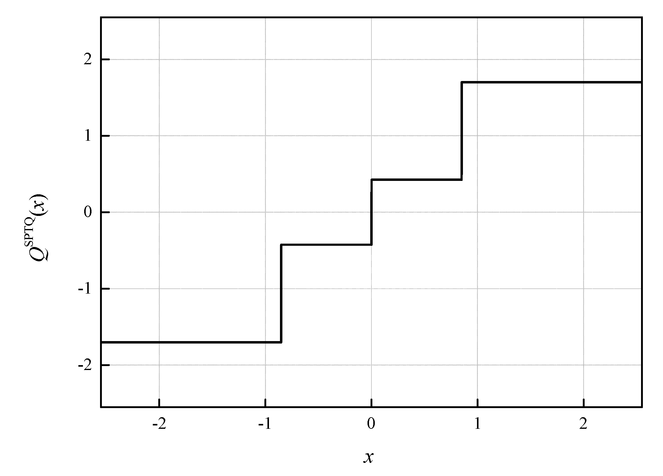In other words, the quantizer in question is completely determined by knowing the support region threshold, x_max = x_max^SPTQ. Therefore, we introduce the following notation of our transfer characteristic of the symmetric two-bit SPTQ, Q^SPTQ(x; x_max) (see Figure 2, where the characteristic of the symmetric two-bit SPTQ is presented for x_max = 2.5512, where the notation [J] comes from the name of the author of [20]).

Let us highlight here that due to the symmetry of the unrestricted Laplacian pdf, p(x) of zero mean and variance σ² = 1

$$p(x)=\frac{1}{\sqrt{2}}\exp \left\{-\sqrt{2}x\right\}$$

(9)

for which we intend to optimize the design of our SPTQ, the decision thresholds and representation levels of SPTQ are assumed to be symmetric in relation to the zero-mean value.

To determine the total distortion of our symmetrical two-bit SPTQ, composed of the granular and the overload distortion, $D_{}^{\mathrm{SPTQ}}=D_{\mathrm{g}}^{\mathrm{SPTQ}}+D_{\mathit{o}}^{\mathrm{SPTQ}}$, we begin with the basic definition of distortion, given by Equation (1) [20], where the granular distortion, $D_{\mathrm{g}}^{\mathrm{SPTQ}}$, and the overload distortion, $D_{\mathrm{o}}^{\mathrm{SPTQ}}$, for symmetric two-bit SPTQ in question are:

$$D_{\mathrm{g}}^{\mathrm{SPTQ}}=2{\displaystyle \sum _{i=1}^2{\displaystyle \underset{x_{i-1}}{\overset{x_i}{\int }}{\left(x-y_i\right)}^{2}p\left(x\right)}}dx$$

(10)

$$D_{\mathrm{o}}^{\mathrm{SPTQ}}=2{\displaystyle \underset{x_2}{\overset{\infty }{\int }}{\left(x-y_2\right)}^{2}p\left(x\right)}dx$$

(11)

Foremost, to simplify our derivation, let us define that it holds x₃ = ∞, denoting the upper limit of the integral in Equation (11). Then, the total distortion of our symmetrical two-bit SPTQ can be rewritten as:

$$\begin{array}{l}{D}^{\mathrm{SPTQ}}=2{\displaystyle \sum _{i=1}^3{\displaystyle \underset{x_{i-1}}{\overset{x_i}{\int }}{x}^{2}p\left(x\right)}}dx-4\left({\displaystyle \sum _{i=1}^2{y}_i{\displaystyle \underset{x_{i-1}}{\overset{x_i}{\int }}xp\left(x\right)}}dx+y_2{\displaystyle \underset{x_2}{\overset{\infty }{\int }}xp\left(x\right)}dx\right)\\ \hspace{0.33em}\hspace{0.33em}\hspace{0.33em}\hspace{0.33em}\hspace{0.33em}\hspace{0.33em}\hspace{0.33em}\hspace{0.33em}\hspace{0.33em}+2\left({\displaystyle \sum _{i=1}^2{y}_i{}^2{\displaystyle \underset{x_{i-1}}{\overset{x_i}{\int }}p\left(x\right)}}dx+y_2{}^2{\displaystyle \underset{x_2}{\overset{\infty }{\int }}p\left(x\right)}dx\right)\end{array}$$

(12)

For the Laplacian pdf, specified in Equation (9), from Equation (12), we derive:

$$D^{\mathrm{SPTQ}}=1-\sqrt{2}\left[y_1+\left(\sqrt{2}{x}_1+1\right)\exp \left\{-\sqrt{2}{x}_1\right\}\left(y_2-y_1\right)\right]+y_1^2+\exp \left\{-\sqrt{2}{x}_1\right\}\left(y_2^2-y_1^2\right)$$

(13)

By further reorganizing Equation (13), we have:

$$D^{\mathrm{SPTQ}}=1+y_1{}^2-\sqrt{2}{y}_1+\left[\left(y_2-y_1\right)\left(y_2+y_1-2x_1-\sqrt{2}\right)\right]\exp \left\{-\sqrt{2}{x}_1\right\}$$

(14)

Eventually, by substituting Equations (7) and (8) into Equation (14), we derive:

$$D^{\mathrm{SPTQ}}=1-\frac{\sqrt{2}}{2}\Delta +\frac{{\Delta }^2}{4}+\left[\frac{3}{4}{\Delta }^2-\frac{3\sqrt{2}}{2}\Delta \right]\exp \left\{-\sqrt{2}\Delta \right\}$$

(15)

By minimizing distortion, that is, by setting the first derivative of so obtained distortion, D^SPTQ, with respect to Δ equal to zero:

$$\frac{\partial D^{\mathrm{SPTQ}}}{\partial \Delta }=0$$

(16)

we derive:

$$\Delta -\sqrt{2}+\left(\frac{3\sqrt{2}}{2}{\Delta }^2-9\Delta +3\sqrt{2}\right)\exp \left\{-\sqrt{2}\Delta \right\}=0$$

(17)

and we determine Δ iteratively from:

$${\Delta }^{\left(i+1\right)}=\sqrt{2}+\left(\frac{3\sqrt{2}}{2}{\left({\Delta }^{(i)}\right)}^2-9{\Delta }^{(i)}+3\sqrt{2}\right)\exp \left\{-\sqrt{2}{\Delta }^{(i)}\right\}$$

(18)

Taking a second derivative of D^SPTQ with respect to Δ yields:

$$\frac{{\partial }^2{D}^{\mathrm{SPTQ}}}{\partial {\Delta }^2}=\frac{1}{2}\left[1+3\exp \left\{-\sqrt{2}\Delta \right\}\left({\left(\Delta -2\sqrt{2}\right)}^2-3\right)\right]$$

(19)

It is trivial to conclude that for $\Delta \le 2\sqrt{2}-\sqrt{3}$ and $\Delta \ge 2\sqrt{2}+\sqrt{3}$ it stands that ${\partial }^2{D}^{\mathrm{SPTQ}}/\partial {\Delta }^2\ge 1/2$. We will now pay special attention to $2\sqrt{2}-\sqrt{3}<\Delta <2\sqrt{2}+\sqrt{3}$, where we can expect the minimum of ${\partial }^2{D}^{\mathrm{SPTQ}}/\partial {\Delta }^2$. By further taking the derivative of expression (19) with respect to Δ and equating the result to zero.

$$\frac{\partial }{\partial \Delta }\left[\frac{1}{2}\left[1+3\exp \left\{-\sqrt{2}\Delta \right\}\left({\left(\Delta -2\sqrt{2}\right)}^2-3\right)\right]\right]=0$$

(20)

we derive:

$${\Delta }^2-5\sqrt{2}\Delta +9=0$$

(21)

and we determine the roots of Equation (21) as ${\Delta }_{1,2}=\left(5\pm \sqrt{7}\right)/\sqrt{2}$. As for ${\Delta }_2=\left(5+\sqrt{7}\right)/\sqrt{2}$ the inequality does not apply $2\sqrt{2}-\sqrt{3}<\Delta <2\sqrt{2}+\sqrt{3}$, the minimal value of ${\partial }^2{D}^{\mathrm{SPTQ}}/\partial {\Delta }^2$ is achieved for ${\Delta }_1=\left(5-\sqrt{7}\right)/\sqrt{2}$ and amounts to 0.263. Thus, we can conclude that D^SPTQ is a convex function of Δ. Moreover, to confirm that we end up iteratively with the unique optimal value for Δ in the numerical result section, we provide the results of numerical distortion optimization per Δ.

4. Symmetric MSPTQ Design for the Laplacian Source

Let us assume the same quantization rule [−3Δ, 3Δ] as in the SPTQ design for specifying the support region of MSPTQ, [−3Δ^mod, 3Δ^mod], as well as the same rule for specifying the representation levels, here denoted with $y_1^{\mathrm{mod}}$ and $y_2^{\mathrm{mod}}$

$$y_i^{\mathrm{mod}}=(2^{i-1}+2^{i-2}-1){\Delta }^{\mathrm{mod}},\hspace{0.33em}{y}_{-i}^{\mathrm{mod}}=-y_i^{\mathrm{mod}}=, i\in \left\{\hspace{0.33em}1,\hspace{0.33em}2\right\}$$

(22)

where mod indicates modification. Let us further assume an additional specification of MSPTQ that quantizer decision threshold is centered between the nearest representation levels (similarly as in the UQ design):

$$x_1^{\mathrm{mod}}=\frac{y_1^{\mathrm{mod}}+y_2^{\mathrm{mod}}}{2}$$

(23)

We should highlight that the spreading of the first quantization cell in MSPTQ, nearest to the mean, causes shrinkage of the adjacent quantization cell (see Figure 3), whereas the common quantization rule of both quantizers in question that the quantization support region ranges [−3Δ, 3Δ] or [−3Δ^mod, 3Δ^mod] is preserved. More precisely, the condition stated in Equation (23), previously mentioned as the additional specification, is one of the prerequisites for the MSPTQ design. To completely specify MSPTQ, it is necessary to determine the quantization step size Δ^mod. To do so, we can minimize the distortion of MSPTQ having the support region that ranges [−3Δ^mod, 3Δ^mod]. For the given x_max^MSPTQ = 3Δ^mod = $x_2^{\mathrm{mod}}$ according to Equations (22) and (23), we can determine the code book $Y^{\mathrm{MSPTQ}}\equiv \left\{y_{-2}^{\mathrm{mod}},y_{-1}^{\mathrm{mod}},y_1^{\mathrm{mod}},y_2^{\mathrm{mod}}\right\}\subset ℝ$ of our two-bit MSPTQ and the decision threshold $x_1^{\mathrm{mod}}$. Let us highlight again that symmetry about zero-mean value holds, so that by specifying $x_0^{\mathrm{mod}}=0$, and identifying that $x_{-i}^{\mathrm{mod}}=-x_i^{\mathrm{mod}},i\in \left\{\hspace{0.33em}1,\hspace{0.33em}2\right\}$, MSPTQ is completely determined. To clearly distinguish the two NUQ models we have proposed in this paper, in

Table 1. The decision thresholds and representation levels of our two-bit (a) SPTQ and (b) MSPTQ.

Quantizer type	x0	x1	x2 = xmaxSPT	y1	y2
SPTQ	0	Δ	3Δ	1/2Δ	2Δ
(a)
Quantizer type	x0mod	x1mod	x2mod= xmaxMSPTQ	y1mod	y2mod
MSPTQ	0	5/4 Δmod	3Δmod	1/2Δmod	2Δmod
(b)

we summarize the main parameters that unambiguously describe our NUQs, SPTQ (Table 1a)) and MSPTQ (Table 1b)). Note that the representation levels of SPTQ and MSPTQ follow the same rule y₁ = Δ/2, y₁^mod = Δ^mod/2 and y₂ = 2Δ, y₂^mod = 2Δ^mod, where the main difference is in specifying the decision thresholds $x_1^{}$ and $x_1^{\mathrm{mod}}$.

Let us specify the distortion of MSPTQ. By recalling the Equation (14) and applying the condition specified in Equation (23), we have:

$$D^{\mathrm{MSPTQ}}=1+{\left(y_1^{\mathrm{mod}}\right)}^2-\sqrt{2}{y}_1^{\mathrm{mod}}-\left[\sqrt{2}\left(y_2^{\mathrm{mod}}-y_1^{\mathrm{mod}}\right)\right]\exp \left\{-\sqrt{2}{x}_1^{\mathrm{mod}}\right\}$$

(24)

By further rearranging Equation (24), so that it only depends on Δ^mod and not on the representation and decision levels, we can derive the expression for the distortion as:

$$D^{\mathrm{MSPTQ}}=1+\frac{{\left({\Delta }^{\mathrm{mod}}\right)}^2}{4}-\frac{\sqrt{2}}{2}{\Delta }^{\mathrm{mod}}\left[1+3\exp \left\{-\frac{5\sqrt{2}{\Delta }^{\mathrm{mod}}}{4}\right\}\right]$$

(25)

By minimizing the distortion, that is by setting the first derivative of obtained distortion in Equation (25) with respect to Δ^mod equal to zero:

$$\frac{\partial D^{\mathrm{MSPTQ}}}{\partial {\Delta }^{\mathrm{mod}}}=0$$

(26)

we derive:

$$\frac{{\Delta }^{\mathrm{mod}}}{\sqrt{2}}\left(15+2\exp \left\{\frac{5\sqrt{2}{\Delta }^{\mathrm{mod}}}{4}\right\}\right)-\left(6-2\exp \left\{\frac{5\sqrt{2}{\Delta }^{\mathrm{mod}}}{4}\right\}\right)=0$$

(27)

Δ^mod can be determined iteratively from:

$${\Delta }^{\mathrm{mod}}{}^{{}^{\left(i+1\right)}}=\sqrt{2}\left(1-\frac{9}{15+2\exp \left\{\frac{5\sqrt{2}{\Delta }^{{\mathrm{mod}}^{\left(i\right)}}}{4}\right\}}\right)$$

(28)

By determining Δ^mod we can calculate the total distortion of the MSPTQ from Equation (25).

Let us determine the second derivative of so obtained distortion, with respect to Δ^mod:

$$\frac{{\partial }^2{D}^{\mathrm{MSPTQ}}}{\partial {\left({\Delta }^{\mathrm{mod}}\right)}^2}=\frac{1}{2}\left[1+\left(15-\frac{75\sqrt{2}}{8}\right)\exp \left\{-\frac{5\sqrt{2}{\Delta }^{\mathrm{mod}}}{4}\right\}\right]$$

(29)

As it holds that $15-75\sqrt{2}/8>0$ and, therefore, ${\partial }^2{D}^{\mathrm{MSPTQ}}/\partial {\left({\Delta }^{\mathrm{mod}}\right)}^2\ge 1/2$, we can conclude that D^MSPTQ is a convex function of Δ^mod, which guarantees the existence of the unique minimum of D^MSPTQ. As in the case of SPTQ, to confirm that we end up iteratively with the unique optimal value for Δ^mod, in the numerical result section, we provide the results of numerical distortion optimization per Δ^mod.

5. Application of Two Novel Non-Uniform Quantizers in Post-Training Quantization

The MNIST handwritten digits database [26] was used in [18,19] for the experimental evaluation of the post-training low-bit UQ performance in weights compression of the three-layer fully connected (FC) NN model (shortly, our NN model). We chose to work with the MNIST dataset as it provides a large number of handwritten digit instances, which is a prerequisite for the highly accurate NNs. We consider that it is interesting to research whether with QNN this high accuracy can be preserved. More precisely, the MNIST dataset consists of 70,000 grayscale images, divided as 60,000 training images and 10,000 images in the test set [26,27], while these sets do not have overlapping instances. All the images used for training and testing the NN are previously standardized and normalized according to their mean value and standard deviation so the pixel values, ranging between 0 and 255, are mapped to a range between 0 and 1. Each image contains 28 × 28 pixels with a size-normalized digit or number (0–9). All digits are positioned in a fixed size with the intensity at the center.

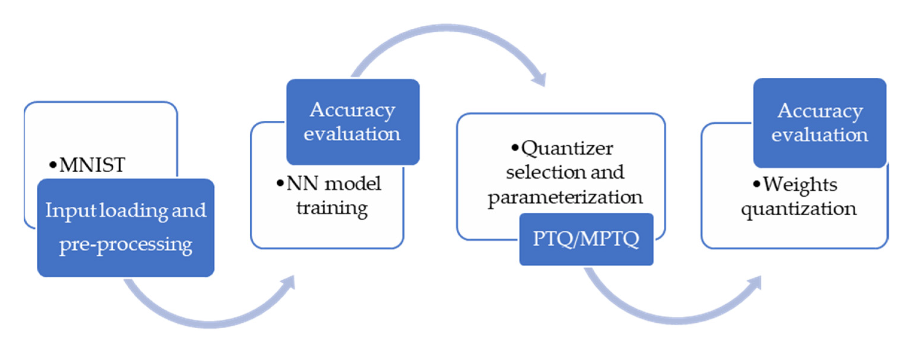
Figure 4 illustrates the process of our experiments: MNIST training and testing datasets are loaded and then reshaped (flattened) into 1-dimensional vectors of 784 (28*28) elements. Each component of the vector is a binary value, which specifies the intensity of the pixel. Our NN model architecture is the same as those specified in [18,19] for comparison reasons and it consists of three FC (Dense) layers. First two FC layers consist of 512 nodes, where the first layer accepts an input shape of (784). These layers are called the hidden layers, as we do not directly consider their outputs. After both hidden layers ReLU activation function is applied. To reduce overfitting, we introduced dropout regularization that randomly sets outputs of 20% of the total nodes in the layer to zero. Output of the second hidden layer is fed to the output layer, which consists of ten neurons that determine the input digit in the range from 0 to 9. Since the output layer uses SoftMax as an activation function, it classifies the output digit according to the highest probability value of the SoftMax function at the output layer [28].

Training and accuracy evaluation of our NN model is implemented in TensorFlow framework with Keras API, version 2.5.0 [28]. Our MLP model consists of 669,706 trainable parameters, which are quantized by using the two-bit novel NUQs after training. Training is conducted in 10 epochs, with a batch size of 128, resulting in 469 iterations per epoch to complete the training over 60,000 training examples. The validation set accuracy after the training amounts to 0.981, meaning that the MLP model made accurate predictions for 98.1% of the images in the validation set. It is well-known that different sizes of the fully connected layers would result in different accuracies obtained. Although NN with a large number of layers and a lot of hidden neurons per layer can achieve better accuracy, smaller NNs run much faster. As already mentioned in this paper, we use the same three-layer FC MLP model as in [18,19]. Our goal is to test the performance of two novel NUQs in post-training quantization and to provide a fair comparison with the results from [18,19].

For the specified NN model, training, accuracy analysis and quantization have been implemented in Python programming language [28]. In our QNN model, all trained weights have been quantized using one of the proposed novel NUQs (SPTQ or MSPTQ) and our QNN model’s accuracy, as well as SQNR, has been evaluated for compressed/quantized weights to represent post-training two-bit NUQ (SPTQ or MSPTQ) performance (see Algorithm 1). We can evaluate the experimental performance of SPTQ and MSPTQ by determining the distortion or SQNR, defined similarly as in [19]:

$$D_{\mathrm{ex}}^{*}=\frac{1}{W}{‖\widehat{W}-{\widehat{W}}^{*}‖}_2^2=\frac{1}{W}{\left(\widehat{W}-{\widehat{W}}^{*}\right)}^{\mathrm{T}}\left(\widehat{W}-{\widehat{W}}^{*}\right)=\frac{1}{W}{\displaystyle \sum _{j=1}^W{\left(w_j-w_j^{*}\right)}^2}$$

(30)

$${\mathrm{SQNR}}_{\mathrm{ex}}^{*}=10{\log }_{10}\left(\frac{\frac{1}{W}{\displaystyle \sum _{j=1}^W{w}_j^2}}{D_{\mathrm{ex}}^{*}}\right)$$

(31)

where * refers to the application of SPTQ or MSPTQ. D_ex^* and SQNR_ex^* are experimentally determined distortion and SQNR, Ŵ = {w_j}_{j = 1, 2, …, W} denotes the vector of weights represented in FP32 format and Ŵ^*= {w_j^*}_{j = 1, 2, …, W} denotes the vector of weights to be loaded in QNN. In brief, at the very beginning of the post-training quantization, NN weights are normalized to zero mean and unit variance, forming the vector Ŵ^N= {w_j^N}_{j = 1, 2, …, W}. After all normalized weights are quantized by applying SPTQ or MSPTQ and denormalized to the original range, Ŵ^* = {w_j^*}_{j = 1, 2, …, W} is loaded into the QNN model (see Algorithm 1).

Algorithm 1: Weights compression by means of post-training quantization using SPTQ/MSPTQ

Notation: wj—pretrained weight, wjSPTQ—quantized weight using SPTQ, wjMSPTQ—quantized weight using MSPTQ Input: Ŵ = {wj}j = 1, 2, …, W, weights represented in FP32 format, εmin = 10−4 Output: Quantized weights for SPTQ—ŴSPTQ = {wjSPTQ}j = 1, 2, …, W, Quantized weights for MSPTQ—ŴMSPTQ = {wjMSPTQ}j = 1, 2, …, W, ${\mathrm{SQNR}}_{\mathrm{th}}^{\mathrm{SPTQ}}$, ${\mathrm{SQNR}}_{\mathrm{ex}}^{\mathrm{SPTQ}}$, ${\mathrm{SQNR}}_{\mathrm{th}}^{\mathrm{MSPTQ}}$, ${\mathrm{SQNR}}_{\mathrm{ex}}^{\mathrm{MSPTQ}}$, AccuracySPTQ, AccuracyMSPTQ Algorithm steps: 1: load initial pretrained and stored weights Ŵ = {wj}j = 1, 2, …, W 2: normalize weights and form ŴN = {wjN}j = 1, 2, …, W, 3: wmin← minimal value of the normalized weights from ŴN 4: wmax ← maximal value of the normalized weights from ŴN 5: select SPTQ model to quantize normalized weights 6:  initialize εSPTQ ← 1, Δ(0) = ΔSPTQ ← 1 (or some other given value), i ← 1 7:  while εSPTQ ≥ εmin do 8:  calculate Δ(i + 1) by using (18) 9:  calculate εSPTQ =abs (Δ(i + 1)-ΔSPTQ) 10:   ΔSPTQ ← Δ(i + 1) 11:  i ← i + 1 12:  end while 13:  Δ ← ΔSPTQ 14:   xmaxSPTQ ← 3 Δ 15:  calculate {x-2, x-1, x0, x1, x2} by using (7) for xmaxSPTQ 16:   form codebook YSPTQ = {y-2, y-1, y1, y2} by using (8) or Table 1a) 17: quantize normalized weights by using codebook YSPTQ 18: denormalize quantized weights and form vector ŴSPTQ = {wjSPTQ}j = 1, 2, …, W 19: select MSPTQmodel to quantize normalized weights 20: initialize εMSPTQ ← 1, Δmod(0) = ΔMSPTQ ← ΔSPTQ, i ← 1 21: while εMSPTQ ≥ εmin do 22: calculate Δmod(i + 1) by using (28) 23: calculate εMSPTQ =abs (Δmod(i + 1)-ΔMSPTQ) 24: ΔMSPTQ ← Δmod(i + 1) 25: i ← i + 1 26: end while 27:  Δmod ← ΔMSPTQ 28: xmaxMSPTQ ← 3 ΔMSPTQ 29: calculate {x-2mod, x-1mod, x0mod, x1mod, x2mod} by using Table 1b) for xmaxMSPTQ 30: form codebook YMSPTQ ≡ {y-2mod, y-1mod, y1mod, y2mod} by using Table 1b) 31: quantize normalized weights by using codebook YMSPTQ 32: denormalize quantized weights and form vector ŴMSPTQ = {wjMSPTQ}j = 1, 2, …, W 33: calculate ${\mathrm{SQNR}}_{\mathrm{ex}}^{\mathrm{SPTQ}}$, ${\mathrm{SQNR}}_{\mathrm{th}}^{\mathrm{SPTQ}}$, ${\mathrm{SQNR}}_{\mathrm{ex}}^{\mathrm{MSPTQ}}$, ${\mathrm{SQNR}}_{\mathrm{th}}^{\mathrm{MSPTQ}}$ by using Equations (15), (25), (30)–(33), estimate accuracies of QNNs.

Let us finally define the theoretical SQNR as:

$${\mathrm{SQNR}}_{\mathrm{th}}^{\mathrm{SPTQ}}=10{\log }_{10}\left(\frac{1}{D^{\mathrm{SPTQ}}}\right)$$

(32)

$${\mathrm{SQNR}}_{\mathrm{th}}^{\mathrm{MSPTQ}}=10{\log }_{10}\left(\frac{1}{D^{\mathrm{MSPTQ}}}\right)$$

(33)

which will also be calculated and compared with the experimentally determined SQNR. Recall that D^SPTQ and D^MSPTQ are specified by Equations (15) and (25), respectively.

Additional results are also provided in the paper for specified NN trained on the Fashion-MNIST dataset [29]. Fashion-MNIST is a dataset comprising of 28 × 28 grayscale images of 70,000 fashion products from 10 categories, with 7000 images per category [29]. The training set has 60,000 images and the test set has 10,000 images. Fashion-MNIST shares the same image size, data format and the structure of training and testing splits with the MNIST. It has been highlighted in [30] that although Fashion-MNIST dataset poses a more challenging classification task, compared to MNIST dataset, the usage of MNIST dataset does not seem to be decreasing. Moreover, it has been pointed out at the fact that the reason MNIST dataset is still widely utilized comes from its size, allowing deep learning researchers to quickly check and prototype their algorithms.

The CNN model, also considered in the paper, consists of one convolutional layer, followed by ReLU activation, max pooling and flatten layer, whose output is fed to the previously described MLP with two hidden FC layers and the output layer. The images for MLP are being flattened into 1-dimensional vectors of 784 (28 × 28) elements to match the shape accepted by our first NN, while for a proper CNN input, one additional dimension is being added to represent the channel. Convolutional layer contains 16 filters with kernel size set to 3 × 3, while the max pooling layer utilizes a pooling window of size 2 × 2. The output of the pooling layer is further flattened into a one-dimensional vector for feeding it forward to the FC dense layer. The only difference between the previously described MLP and the dense layers utilized in CNN is in the dropout percentage, which is in the case of CNN set to 0.5, to further prevent overfitting of the FC layers. Therefore, the CNN model consists of three hidden layers and the output layer with the total of 1,652,906 trainable parameters. The training is performed for the Fashion-MNIST, in the same manner as for the MLP, with the total of 10 epochs, while the batch size is equal to 128 training samples.

6. Numerical Results and Analysis

Referencing Algorithm 1 for both previously described novel NUQs, we firstly analyze the number of necessary iterations for iterative determination of Δ and Δ^mod, or equally, for determining x_max^SPTQ and x_max^MSPTQ. To initialize Algorithm 1 for determining Δ, we use different values of Δ⁽⁰⁾, specified in

Table 2. Number of iterations for determining x_max^SPTQ for different initializations.

SPTQ	Δ(0) = 1	Δ(0) = |wmax|/3	Δ(0) = |wmin|/3	Δ(0) = xmax[H]/3	Δ(0) = xmax[J]/3
number of iterations	40	39	40	41	41

. To determine Δ^mod, we use the result of the first iterative process, that is, we assume Δ^mod(0) = Δ. The same condition as in [22], that two adjacent iterations differ by less than 10⁻⁴ is used as the output criterion of algorithm. By observing statistics of the trained and normalized NN weights, we have found that the minimum and maximum weights in original FP32 amount to w_min = ™7.063787 and w_max = 4.8371024. Following a predefined rule for specifying the support region of SPTQ ranging in [−3Δ, 3Δ], we use Δ⁽⁰⁾ = |w_max|/3 = 1.61237 and Δ⁽⁰⁾ = |w_min|/3 = 2.3546 to initialize Algorithm 1 for SPTQ. Moreover, we assume that Δ⁽⁰⁾ = x_max[H]/3 = 0.6536 and Δ⁽⁰⁾ = x_max[J]/3 = 0.7249, where x_max[H] and x_max[J] are optimal and asymptotically optimal x_max values for UQ given by Hui [23] and Jayant [20] (see Table 2). It is worthy highlighting that different initializations require around 40 iterations (see Table 2 and Figure 5). Moreover, we should highlight that all the observed initializations lead to the unique final value of Δ (Δ = 0.8504) and x_max^SPTQ = 3Δ = 2.5512. If we further use Δ^mod(0) = Δ = 0.8504 for iteratively determining Δ^mod, given the same output algorithm criterion, we only need seven iterations. As a result of the second iterative process, we determine Δ^mod = 0.9021, as well as x_max^MSPTQ = 3Δ^mod = 2.7063. To additionally confirm that with the output criterion of Algorithm 1 we ended up with the optimal values for Δ and Δ^mod; one can observe in Figure 6, the depiction of the dependences of the distortion of the applied quantizers on the corresponding basic step sizes. Iteratively obtained values for Δ and Δ^mod are marked with asterisks in Figure 6 and are indeed optimal as they give the minimum of D^SPTQ and D^MSPTQ.

Further in this section, we present experimentally obtained results of applying both SPTQ and MSPTQ in post-training quantization of NN model’s weights. As mentioned, we utilize the same NN model as in [18,19] with the same weights stored in FP32 format. Therefore, by conducting experiments with the novel NUQs, we can fairly compare the performance with the case of applying two-bit UQ under the same circumstances. To analyze the performance of the proposed quantizers in NN quantization, we conduct experiments for multiple specific choices of the support region threshold of NUQs. These experiments aim to provide insights on the impact of different support region thresholds on both NUQs performance and QNN accuracy.

The support region in our Case 1 is defined as [−min(|w_min|,|w_max|), min(|w_min|,|w_max|)], which is in our experiment simply [−w_max, w_max]. Therefore, in Case 1, the support region depends on the maximum value of the normalized trained model weights in full precision, which for the observed trained weights (for MNIST dataset) amounts to w_max = 4.8371024. By setting the support region of SPTQ and MSPTQ as stated, it includes 99.988% of all the normalized weights. One can notice from

Table 3. SQNR and QNN model’s accuracy for MLP trained on MNIST dataset: different SPTQ designs for R = 2 bit/sample.

wmin = −7.063787, wmax = 4.8371024, 3Δ = 2.5512 xmax[H] = 1.9605, xmax[J] = 2.1748	Case 1 ℜg [−wmax, wmax]	Case 2 ℜg [wmin, −wmin]	Case 3 ℜg [−3Δ, 3Δ]	Case 4 ℜg [−xmax[H], xmax[H]]	Case 5 ℜg [−xmax[J], xmax[J]]
SQNRexSPTQ(dB)	4.6899	2.5745	7.8099	7.9051	8.0068
SQNRthSPTQ(dB)	4.4438	1.6044	6.9790	6.5437	6.8086
Accuracy (%)	97.61	97.42	95.75	93.77	94.52
Within ℜg (%)	99.988	100	98.567	94.787	96.691

that thus defined Case 1 provides the highest QNN model’s accuracy of all the observed cases, amounting to 97.61% of correctly classified validation samples of MNIST dataset. By comparing it to the application of simple UQ, we can conclude that with the applied SPTQ, we provide an increase in the accuracy of 0.64% (see

Table 4. SQNR and QNN model’s accuracy for MLP trained on MNIST dataset with the application of different UQ designs for bit rate of R = 2 bit/sample (part of the results are from [18]).

wmin = −7.063787, wmax = 4.8371024, 3Δ = 2.5512 xmax[H] = 1.9605, xmax[J] = 2.1748	Case 1 ℜg [−wmax, wmax]	Case 2 ℜg [wmin, −wmin]	Case 3 ℜg [−3Δ, 3Δ]	Case 4 ℜg [−xmax[H], xmax[H]]	Case 5 ℜg [−xmax[J], xmax[J]]
SQNRexUQ(dB)	2.8821	™1.2402	8.2325	8.7676	8.7639
SQNRthUQ(dB)	1.9360	™2.0066	6.8237	6.9787	7.0707
Accuracy (%)	96.97	94.58	97.12	96.34	96.74
Within ℜg (%)	99.988	100	98.567	94.787	96.691

). This represents a significant increase in accuracy, especially taking into account that the only difference is in the applied quantizers, while the same bit rate is assumed and we are very close to the full precision accuracy of the baseline NN. Similarly, the experimental and theoretically obtained SQNR of SPTQ is higher, compared to UQ, providing gain in SQNR of 1.8078 dB and 2.5078 dB, respectively. We can notice that theoretically determined SQNR has lower values than experimentally determined SQNR. As explained in [18,19], the reason is that in the experimental analysis, the weights originating from the Laplacian-like distribution being quantized are from the limited set of possible values [−7.063787, 4.8371024] (see Figure 7), while in the theoretical analysis, the quantization of values from the unrestricted Laplacian source is assumed, causing an increase in the amount of distortion, that is, the decrease in the theoretical SQNR value. In summary, Case 1 already shows the benefits of implementing SPTQ over the UQ providing increase in all significant performance indicators observed.

In Case 2, the support region is [−max(|w_min|, |w_max|), max(|w_min|, |w_max|)], and it is defined as it is in [31]. In our experiment, it can be expressed as [−|w_min|, |w_min|], which in practice becomes [w_min, −w_min], forming the support region (in case of MNIST dataset) as [−7.063787, 7.063787]. It can be observed that the support region in Case 2 includes 100% of the weights and even goes beyond the maximum value of the normalized weights, which makes it unnecessarily wide and representative of an unfavorable choice of ℜ_g.

Therefore, in this case we obtain the lowest observed SQNR value among all cases, while being significantly higher than the one obtained by UQ, which reaches negative values. Unlike the low SQNR value, the accuracy in Case 2 is very high with 97.42% achieved, especially taking into consideration that for UQ observed in the same case, the accuracy amounts to only 94.58%. This highlights the benefits of utilizing non-uniform quantization, which provides better QNN performance even in the case of choosing an overly wide support region.

In Case 3, the support region, ℜ_g, is determined for the iteratively calculated optimal quantization step, Δ = 0.8504. The support region threshold of SPTQ is defined as follows:

x_max^SPTQ = 3Δ, and x_max^SPTQ amounts to 2.5512. This value represents the theoretically optimal support region threshold value, therefore, providing the maximal theoretical SQNR value for this case. Although Case 3 yields the highest theoretical and higher experimental SQNR, compared to the previous cases, the QNN model’s accuracy is significantly lower. This further confirms the premise that the quantizer that provides the highest SQNR does not necessarily provide the highest accuracy of the QNN, which highly depends on the ℜ_g choice as well.

Cases 4 and 5 utilize well-known, optimal and asymptotically optimal support region thresholds from the literature, which are determined for UQ by Hui [23] and Jayant [20]. Although these values are not optimal for our SPTQ, we include them into our analysis to obtain a better insight on the influence of the ℜ_g choice to both SQNR and QNN performance. One can notice that although not optimal for SPTQ, support region thresholds specified in Cases 4 and 5 provide the highest experimental SQNR values, with theoretical SQNR being relatively close to the optimal value with the maximum difference from it of about 0.4 dB. Unlike SQNR, in these two cases we obtain the lowest QNN model’s accuracy. The maximum accuracy difference in these two cases is about 4%, compared to the best performing Case 1, which represents a significant NN performance degradation. Lower accuracy is a direct result of overly narrow support region threshold, with 94.787% and 96.691% of the weights being within the ℜ_g for the Cases 4 and 5, respectively.

By analyzing all the observed cases, one can conclude that ℜ_g has a very strong influence on the QNN accuracy and obtained SQNR. Moreover, it has been shown that SPTQ performs much better than UQ for the case of using wider ℜ_g, which we intuitively expected, and it is generally known for non-uniform quantization [20]. In contrast, it can be observed that the accuracy of the QNN with the application of UQ outperforms the QNN with SPTQ in Cases 3–5, with Case 3 being the most significant one, as it represents the optimal solution for the theoretical SQNR of the SPTQ. Based on the SQNR analysis of SPTQ, we can conclude that SPTQ designed in Case 3 could be greatly applicable in traditional quantization tasks. To overcome the mentioned imperfection of SPTQ in post-training quantization, in this paper, we have introduced a simple, yet efficient modification and optimization of the SPTQ, denoted by MSPTQ, which performance is presented and analyzed in the following.

As previously described, MSPTQ introduces a simple modification in specifying one decision threshold to improve the performance of SPTQ for the cases of narrower ℜ_g, including the one constructed with the optimal support region threshold value. The performances of the modified SPTQ and MSPTQ are presented in

Table 5. SQNR and QNN model’s accuracy for MLP trained on MNIST dataset: the application of MSPTQ designs for bit rate of R = 2 bit/sample.

wmin = −7.063787, wmax = 4.8371024, xmaxSPTQ =3Δ = 2.5512 xmaxMSPTQ = 3Δmod = 2.7063	Case 1 ℜg [−wmax, wmax]	Case 2 ℜg [wmin, −wmin]	Case 3 ℜg [−3Δ, 3Δ]	Case 4 ℜg [−3Δmod, 3Δmod]
SQNRexMSPTQ(dB)	5.5741	2.9114	8.6839	8.5608
SQNRthMSPTQ(dB)	5.0581	1.9158	7.4890	7.5165
Accuracy (%)	97.91	96.98	97.17	97.23
Within ℜg (%)	99.988	100	98.567	99.001

for slightly different Cases of the support region threshold, as previously defined Cases 4 and 5 are not relevant to the non-uniform quantization. Cases 1 to 3 are the same as in the previous analysis, so that we can conduct a direct comparison of performance. One can notice that MSPTQ outperforms both SPTQ and UQ in all the observed performance indicators for Cases 1 and 3, while QNN with the application of SPTQ obtains a higher accuracy with the margin of 0.44% for Case 2. Moreover, MSPTQ provides the gain in both theoretical and experimental SNQR values for all comparable cases over the QNN with the implementation of UQ. Case 2 is a specific one, being an example of an unfavorable choice of ℜ_g, and QNN with SPTQ performs better, compared to its modified counterpart. On the other hand, for carefully designed ℜ_g, by applying the modified SPTQ and MSPTQ, we obtain a significant increase in both SQNR and QNN accuracy, compared to the SPTQ. The gain in the accuracy is specifically large in Case 3, which utilizes the support region threshold, optimally determined for SPTQ, and it amounts to 1.42%. For the ℜ_g specified in Case 3, MSPTQ obtains the highest experimental SQNR value, with an increase of 0.874 dB, compared to SPTQ and 0.4514 dB, in comparison to UQ. Case 4 implements the numerically optimized ℜ_g width for the MSPTQ, with the support region threshold value being close to the one obtained for SPTQ. Expectedly, theoretically obtained SQNR is highest for this case, while experimentally obtained SQNR, as well as the accuracy, take the second highest value among all the cases by having 99.001% of the normalized weights within the ℜ_g. As the degradation of the accuracy in Case 4 amounts to about 0.9%, compared to the full precession case (98.1% − 97.23% = 0.87%), we can conclude that with the simple modification we have managed not only to improve SQNR, but also to increase the accuracy of the QNN, compared to the case where UQ and SPTQ are implemented.

We can additionally compare our results with the ones from [16]. In particular, in [16], 2-bit logarithmic quantization of neural network weights has been addressed, where MLP (multilayer perceptron) has also been trained for the MNIST dataset. Specifically, paper [16] addressed a two-bit μ-law logarithmic quantizer, parameterized to achieve increased robustness, which is particularly important for the variance-mismatched scenario, where the designed for and applied to variance of data being quantized do not match. However, by performing normalization, which is commonly applied in NNs, this problem reduces to optimization of the quantizer models, typically for the zero mean and unit variance, as with the ones we address in this paper. Although the robustness of the logarithmic quantizer has been recognized as the main advantage, it has been shown in [16] that the higher robustness causes the lower SQNR, compared to the uniform quantizer in the zero mean and unit variance case (see Figure 13 from [16] for σ = σ_ref, that is, for 20 log10(σ/σ_ref) = 0). In [16], SQNR was calculated for different representative values of parameter, μ, in wide dynamic range of variances. By comparing achieved SQNR values from Table I given in [16] (SQNR = 4.44 dB for μ =255) and SQNR values from our Table 3 and Table 5 (SQNR = 7.8099 dB for SPTQ Case 3 and SQNR = 8.5608 dB for MSPTQ Case 4), we can conclude that with SPTQ and MSPTQ, we have achieved higher SQNR values, compared to μ-law logarithmic quantizer from [16]. This confirms that the advantages of the logarithmic quantizer do not come to the forefront in the case of lower bit rates.

In [32], ternary uniform quantization is considered, where binary coding is used, which we also used in this paper, while in [33], ternary coding is applied. Unlike our previous research [18], in which the design of UQ is optimized for the Laplacian pdf of zero mean and unit variance; in [32], the support region threshold of the ternary quantizer is not optimized. However, by introducing the scale factor, α, in [33], a kind of optimization of the considered ternary quantizer model is performed. In order to provide a fair comparison of our results with those from [32] and [33], we assume the same weights for quantization, the same NN, as well as the same support region threshold settings, as in the case of SPTQ and UQ given in Table 3 and Table 4, where we apply the ternary quantization from [32]. Since the number of cells into which the support region is divided in the case of the ternary quantizer is smaller by one (N = 3) than the case of dividing the same support region in the case of the two-bit UQ (N = 2² = 4), our anticipation was that the ternary quantizer will provide a lower SQNR value, as well as a lower accuracy, compared to UQ, which the numerical results shown in

Table 6. SQNR and QNN model’s accuracy for MLP trained on MNIST dataset: (a) the application of different ternary quantizer designs (b) adaptation of ternary quantizer with the scale factor α.

wmin = −7.063787, wmax = 4.8371024, 3Δ = 2.5512 xmax[H] = 1.9605, xmax[J] = 2.1748	Case 1 ℜg [−wmax, wmax]	Case 2 ℜg [wmin, −wmin]		Case 3 ℜg [−3Δ, 3Δ]	Case 4 ℜg [−xmax[H], xmax[H]]		Case 5 ℜg [−xmax[J], xmax[J]]
SQNRex(dB)	1.6988	0.43		5.7178	6.7273		6.47
SQNRth(dB)	2.7275	1.1827		5.5681	5.7436		5.7762
Accuracy (%)	90.56	24.02		96.58	94.1		95.01
Within ℜg (%)	99.988	100		98.567	94.787		96.691
(a)
xmax = 3/sqrt(2) α ℜg[−xmax, xmax]	Case 1ℜg α = 1/4	Case 2ℜg α = 1/2	Case 3ℜg α = 3/4	Case 4ℜg α = 1	Case 5ℜg α = 5/4	Case 6ℜg α = 3/2	Case 7ℜg α = 7/4
SQNRex(dB)	2.52	5.01	6.6	6.552	5.49	4.28	3.23
SQNRth(dB)	2.1424	4.0509	5.3544	5.7800	5.4708	4.8068	4.0695
Accuracy (%)	22.01	94.37	94.81	94.68	96.49	97.51	97.33
Within ℜg (%)	41.142	72.968	89.17	96.283	98.869	99.648	99.887
(b)

confirm. Namely, Table 6 shows the results of the application of ternary quantization to the NN weights of the considered previously trained MLP, where part of the results, shown in part (a) assumes the same support region, as in the case of optimal UQ (Case 5), asymptotically optimal UQ (Case 4) and optimal SPTQ (Case 3), while part (b) illustrates the importance of choosing the value of the scale factor, α, which serves to scale the entire model of the ternary quantizer with the aim to perform its adaptation. In [20], the optimal support region threshold value for the ternary quantizer is given, which for the assumed Laplace pdf is 3/sqrt(2). By setting α = 1, we indeed determined the highest theoretical value of SQNR for the ternary quantizer. However, as it has been shown in [18], the highest SQNR does not always guarantee the highest accuracy; we have varied the value of the scale factor from 1/4 to 7/4 with steps of 1/4, and we have ended up with the conclusion that, for the observed values of α, the highest accuracy is achieved for α = 3/2, providing the accuracy of the observed QNN that amounts to 97.51%. In short, both of our new models of non-uniform quantizers (SPTQ and MSPTQ) have superior performance (higher SQNR and accuracy), compared to the quantizer models from [32] and [33], which is not only a consequence of the fact that the number of cells in our quantizers is greater by one but also that with the wise distribution of the cell width, as well as the optimization of the support region threshold, we really provided significant step forward in the field of quantization.

Table 7. SQNR and QNN model’s accuracy (MLP and CNN trained on Fashion-MNIST dataset) with the application of (a) SPTQ (b) MSPTQ, designed for bit rate of R = 2 bit/sample.

xmaxSPTQ =3Δ = 2.5512	MLP [−3Δ, 3Δ]		CNN [−3Δ, 3Δ]
SQNRexSPTQ(dB)	7.3242		7.51
SQNRthSPTQ(dB)	6.9790		6.9790
Accuracy (%)	86.05		83.69
Within ℜg (%)	98.112		97.696
(a)
xmaxSPTQ =3Δ = 2.5512 xmaxMSPTQ = 3Δmod = 2.7063	MLP [−3Δ, 3Δ]	MLP [−3Δmod, 3Δmod]	CNN [−3Δ, 3Δ]	CNN [−3Δmod, 3Δmod]
SQNRexMSPTQ(dB)	8.13	8.082	8.12	8.13
SQNRthMSPTQ(dB)	7.4890	7.5165	7.4890	7.5165
Accuracy (%)	87.95	87.42	83	83.72
Within ℜg (%)	98.118	98.552	97.696	98.232
(b)

provides additional results for specified NNs trained on the Fashion-MNIST dataset, for the case of applying the proposed two novel NUQs (SPTQ and MSPTQ). As our MLP model achieves the accuracy of 88.96% on the Fashion-MNIST validation set, obtained after 10 epochs of training, we can conclude that similar to the case of the MNIST dataset, with the application of MSPTQ, we have managed to achieve closer to the accuracy obtained in the full precession case. Moreover, we have managed to preserve the original accuracy to a great extent. In addition, as with the results discussed for MNIST dataset, in quantization of weights of MLP trained on Fashion-MNIST dataset, we have ascertained that the theoretically and experimentally obtained SQNR values achieved with the application of MSPTQ are higher than ones obtained with the application of SPTQ.

Compared to MLP, the CNN model achieves a higher accuracy of 91.53%, obtained on the Fashion-MNIST validation set, with weights also represented in FP32 format. Normalized histogram of weights that are being quantized for CNN trained on Fashion-MNIST dataset is shown in Figure 8. It has been shown in [19] that with the application of optimal three-bit UQ, the accuracy degradation of the quantized CNN model amounts to about 3.5% (91.53% − 87.97% = 3.56%). In the case of applying the two-bit UQ to the same weights of the CNN (trained on Fashion-MNIST), we have calculated an even higher accuracy degradation that amounts to about 9.5% (91.53% − 82.039% = 9.491%). As one can observe from Table 7, for the two novel NUQs, we have ascertained the accuracy of 83.69% and 83.72%, respectively. In other words, we have again overperformed UQ in terms of accuracy, and the mentioned accuracy increased amounts to about 1.7%.

7. Summary and Conclusions

In this paper, we have proposed two novel two-bit NUQs, SPTQ and MSPTQ, which prudently utilize one of the two properties of the simplest UQ, and we have examined whether they are more suitable for application in post-training quantization than UQ. By optimizing the distortion of the proposed NUQs to achieve the highest theoretical SQNR, we have derived formulas for iteratively determining the basic step sizes of both NUQs, Δ and Δ^mod, which is of the utmost importance in traditional quantization. We have proved that the iterative algorithms utilized output the values of Δ and Δ^mod that are indeed optimal, as they match with the corresponding results of numerical distortion optimization per basic step sizes and give the minimum of distortion of SPTQ and MSPTQ. Moreover, the main benefits of this paper are meaningful conclusions that specify the manner in which the performance of the proposed quantizers, as well as the performance of QNNs that have implemented novel NUQs, behave with the basic step sizes. We have also confirmed the premise that the quantizer that provides the highest SQNR does not necessarily provide the highest accuracy of QNN. Finally, with the introduction of MSPTQ model we have managed not only to improve the SQNR, but also to increase the accuracy of the QNN, compared to the case where UQ and SPTQ are implemented. Although UQ is a highly exploited quantizer model due to its intriguing nature and its possibility to be modified to some extent, it is natural to expect that research and development of some modified quantization models will continue to attract the attention of the scientific community.