1. Introduction
Over the past few decades, there have been considerable efforts towards linear systems with parameter uncertainty. Adaptive control has been one of the methods to solve this uncertainty. Among various adaptive control techniques, model reference adaptive control (MRAC) is the most popular and mature method, which provides feedback controller structures and adaptive laws for the control of systems to ensure that the closed-loop signals are bounded and the output or the state of the uncertain plant can asymptotically track the output or the state of the desired reference model, despite the uncertainties of the system parameters [
1,
2].
Fractional calculus has captured the attention of many scientists and engineers working in a variety of fields in recent years [
3,
4,
5,
6,
7]. This is mostly owing to its ability to more accurately model specific physical systems than the traditional integer-order option, such as manipulator systems, multi-area power systems, multisource renewable energy systems, and electrical vehicles [
8,
9,
10,
11,
12]. On the other hand, it is suitable for describing hereditary and memorial properties of various processes for which traditional integer-order differential equations fail to capture relevant phenomena, such as heat conduction and viscoelastic mechanics in materials with memory, and Zika virus transmission [
13,
14,
15,
16,
17,
18]. The expansion of MRAC to fractional-order systems, known as FOMRAC, has been proposed in the literature for more than a decade. Many useful results and applications for FOMRAC are studied based on a single-input single-output (SISO) plant. Among them, Shi et al. [
19] proved the stability of the closed-loop control system strictly based on the continuous frequency distributed model. Then, a fractional-order composite MRAC was developed in [
20] by incorporating the parameter estimate error into the parameter updating law to achieve better performance.
Recently, the FOMRAC for multiple-input-multiple-output (MIMO) systems has been studied in the works of Norelys Aguila-Camacho and Manuel A. Duarte-Mermoud [
21,
22,
23,
24]. For example, in Ref. [
21], they have proposed the standard fractional-order update laws and proved the Lyapunov stability of a fractional-order MIMO MRAC system by using a series of fractional inequalities. In Ref. [
22], they further proved the convergence to zero of the mean value of the squared norm of the output error. In particular, the order of the plant and the adaptive laws in the above results are the same. In Ref. [
24], they proposed the fractional-order update laws whose order is smaller than that of the plant. However, the above results usually require online estimation of multiple unknown parameters, and as the input–output dimension of the FOMRAC system increases, the number of parameters that need to be updated online also increases, which greatly increases the computational burden and limits the practicality of FOMRAC. Therefore, the issue of how to reduce the number of parameters estimated online is a critical problem to be solved for the MIMO FOMRAC system.
In this article, a new FOMRAC framework is proposed for fractional-order multivariable systems with parameter uncertainty. The proposed fractional-order adaptive controller with state feedback depends on a fractional-order nonlinear scalar update law. Specifically, the scalar update law does not change as the input–output dimension changes. The major contributions of this paper can be formulated as follows:
we design a new FOMRAC scheme to handle the parameter uncertainty and to ensure the system error stability and closed-loop signal boundedness;
using the proposed FOMRAC framework, only one parameter online update is needed such that the control scheme is computationally inexpensive;
we conduct a complete theoretical analysis of the boundedness of all signals involved in this adaptive scheme and the convergence to zero of the mean value of the squared norm of the system error for the proposed control architecture;
we verify the effectiveness of this control design by two illustrative numerical examples.
This paper is organized as follows.
Section 2 briefly gives some basic concepts about fractional calculus and some necessary lemmas.
Section 3 presents the FOMRAC problem. The adaptive controller based on a fractional-order scalar update law and the stability analysis for the adaptive control architecture are shown in the main results given in
Section 4.
Section 5 presents two numerical examples to clarify the validity of the proposed approach.
Section 6 contains the conclusions and future works.
2. Preliminaries
This section introduces some fundamental concepts of fractional calculus, as well as some properties of fractional operators that will be used throughout the paper.
Notation. The following notations are used throughout the whole paper. Let R and denote the set of real, non-negative real numbers, respectively. denotes the set of real column vectors, denotes the set of real matrices. The matrix P is symmetric if . denotes the positive definite matrix P. denotes the trace of the matrix A.
Definition 1. Riemann–Liouville fractional integral [
3].
where is the Gamma function. Definition 2. Caputo Fractional Derivative [
3].
with , . The following lemmas will be used to prove the main results in this paper.
Lemma 1 ([
23])
. Let be a vector of differentiable functions. Then, for all , the following relationship holdswhere , and , satisfying . Lemma 2 ([
23])
. Let be a time-varying differentiable matrix. Then, for any time instant , the following relationship holds Lemma 3 ([
22])
. Let be a bounded nonnegative function. If there exists some such thatthen 3. FOMRAC Problem
Consider a fractional-order MIMO plant with parameter uncertainty given by
where
is a measurable state vector,
is the control input and the fractional order
. In addition,
is an unknown constant state matrix capturing the parameter uncertainty in the fractional-order MIMO plant, and
denotes a known control matrix. For the well-posedness of the FOMRAC problem, we assume that the pair
is controllable. Recall that the controllability conditions ensure that the control input
has sufficient access to the internal state to stabilize all unstable modes of a plant.
In addition, the fractional-order reference model is chosen by
where
is a reference state vector,
is Hurwitz and known,
is known and
is bounded and piecewise continuous. It is assumed that
, for all
, represents the desired trajectory for
.
The objective of the FOMRAC is to design a feedback controller such that all the signals remain bounded and, ideally, the state of the uncertain system can track the state of the reference model asymptotically.
Next, define an ideal feedback controller that perfectly eliminates the uncertainty and allows
to follow
as
Here,
,
are the ideal control gains chosen such that the matching conditions
and
hold. Since
is known,
K can be obtained directly from the matching condition (
11). Since
is unknown,
is also unknown.
The actual adaptive controller is an estimate of the ideal controller, with the purpose of approaching the ideal controller in the limit. Let
be the actual adaptive controller, where
is the estimate of
.
Now, define the estimation error as
. Then, the closed-loop plant model can be written as
Let
be the tracking error. Then, the tracking error equation is expressed as
The goal of FOMRAC is changed to design the adaptive laws to adjust in such a way that all the closed-loop signals remain bounded and ideally .
In 2015, Duarte-Mermoud, M. A. et al. [
23] designed the standard fractional-order update laws
where
is a positive definite symmetric matrix satisfying the Lyapunov equation
where
Q∈
is positive definite. Since
is a Hurwitz constant matrix, it follows from converse Lyapunov theory [
25,
26] that, for any given matrix
, there exists a unique matrix
that satisfies the Lyapunov Equation (
16). Recently, Aguila-Camacho, N. et al. [
24] designed the fractional-order update laws for
as
where
. This denotes that the order of the adaptive laws can be smaller than the order of the plant. Specifically, when the plant under control is of integer order, the adaptive laws can be fractional, which is one of the most promising applications from the practical point of view.
In the above works, is an adaption parameter matrix satisfying update laws, where m and n are the dimension of the input and output, respectively. However, as the input–output dimension of the FOMRAC system increases, the number of parameters that need to be updated online also increases, which greatly increases the computational burden of the online part and limits the practicality of FOMRAC. Therefore, how to reduce the number of parameters estimated online is a critical problem to be solved for the MIMO FOMRAC system.
5. Simulation Example
In this section, we present two numerical examples to demonstrate the utility of the proposed adaptive control scheme. The scheme was implemented in Matlab/Simulink, using the FOMCON Toolbox to obtain the required results.
Example 1. Let us consider a MIMO fractional-order linear time-invariant plant with parameter uncertainty, which is given bywhere . Here, is an unknown constant state matrix that denotes the parameter uncertainty. For simulation purposes, the true . For this study, we choose the reference model given by
where
. Consequently, the ideal control gains become
and
.
For this case, matrices and exist such that .
Further, we choose
for the proposed fractional-order nonlinear scalar update law given by (
21). Then, the update law of
is
where
For convenience, the reference signal
is chosen as the unit step signal and the fractional order used is
. Then, we have the following numerical results displayed in
Figure 2,
Figure 3,
Figure 4,
Figure 5 and
Figure 6.
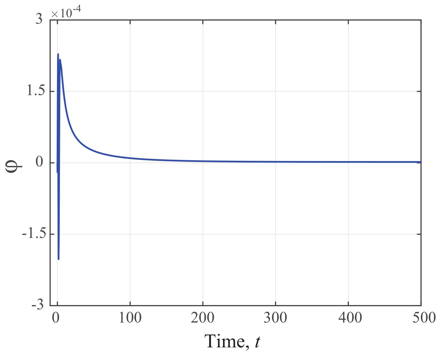
Figure 2,
Figure 3,
Figure 4,
Figure 5 and
Figure 6 show that, as stated by the analysis above, the tracking error, the scalar function
and the system state remain bounded for every
. In addition to the boundedness of the closed-loop signals,
Figure 2 and
Figure 3 show that the tracking error converges to zero, although only the convergence of the mean value of
was analytically proven.
External Disturbance
To illustrate the robustness of the system, we consider that the system (
30) is subject to a parametric variation of the state matrix
in the form
at
t = 20 s, where
and
. Here, we choose
,
, and the simulation results are shown in
Figure 7 and
Figure 8. This example shows that, even in the case of an external disturbance to the system (
30), the proposed FOMRAC scheme maintains its performance and the tracking of the reference model trajectory.
Example 2. Let us consider a fractional-order multivariable system with parameter uncertainty, where , is unknown, and is known and given by , , . For the purpose of simulation, the true . Therefore, the ideal control gain becomes and .
In the simulation, we set matrix and exist such that .
From (
15), (
17) and (
21), we can obtain that
where
, and the number of update laws in the standard fractional-order adaptive controller and the fractional adaptive controller in [
24] is 2, and ours is only 1. Therefore, compared with the other two adaptive controllers, our controller can reduce the number of parameters updated online.
To further demonstrate the efficacy of the proposed adaptive control architecture, we compare the evolution of system state and system error with the standard fractional-order adaptive controller in [
23], the fractional adaptive controller in [
24] and our proposed adaptive controller. The initial values correspond to
,
, the fractional order used is
, and the reference signal
. For convenience, we choose
for the fractional adaptive controller in [
24], and
for our proposed adaptive controller. Then, we have the following numerical results shown in
Figure 9,
Figure 10,
Figure 11 and
Figure 12.
From
Figure 9,
Figure 10,
Figure 11 and
Figure 12, we can find that the standard fractional-order adaptive controller in [
23], the fractional adaptive controller in [
24] and our proposed adaptive controller all can make the tracking error bounded so that
follows
. Moreover, from
Figure 9 and
Figure 10, taking the
error band, we can obtain that the response adjustment times of
and
with the standard fractional-order adaptive controller, the fractional adaptive controller in [
24] and our proposed adaptive controller are 3.1033 s, 2.9814 s, 7.5304 s, and 1.5791 s, 1.029 s, 3.5002 s, respectively. Moreover, the ratio of overshoot of
and
is
:
:0, and
:
:0, respectively. Therefore, compared with the other two fractional-order adaptive controllers, the response adjustment time of our controller is relatively longer, but the overshoot is smaller.
Based on the above analysis, our control architecture can reduce the online computation burden while maintaining the stability of the tracking error.


