

Efficient Numerical Solutions to a SIR Epidemic Model
 ,
,  , , and
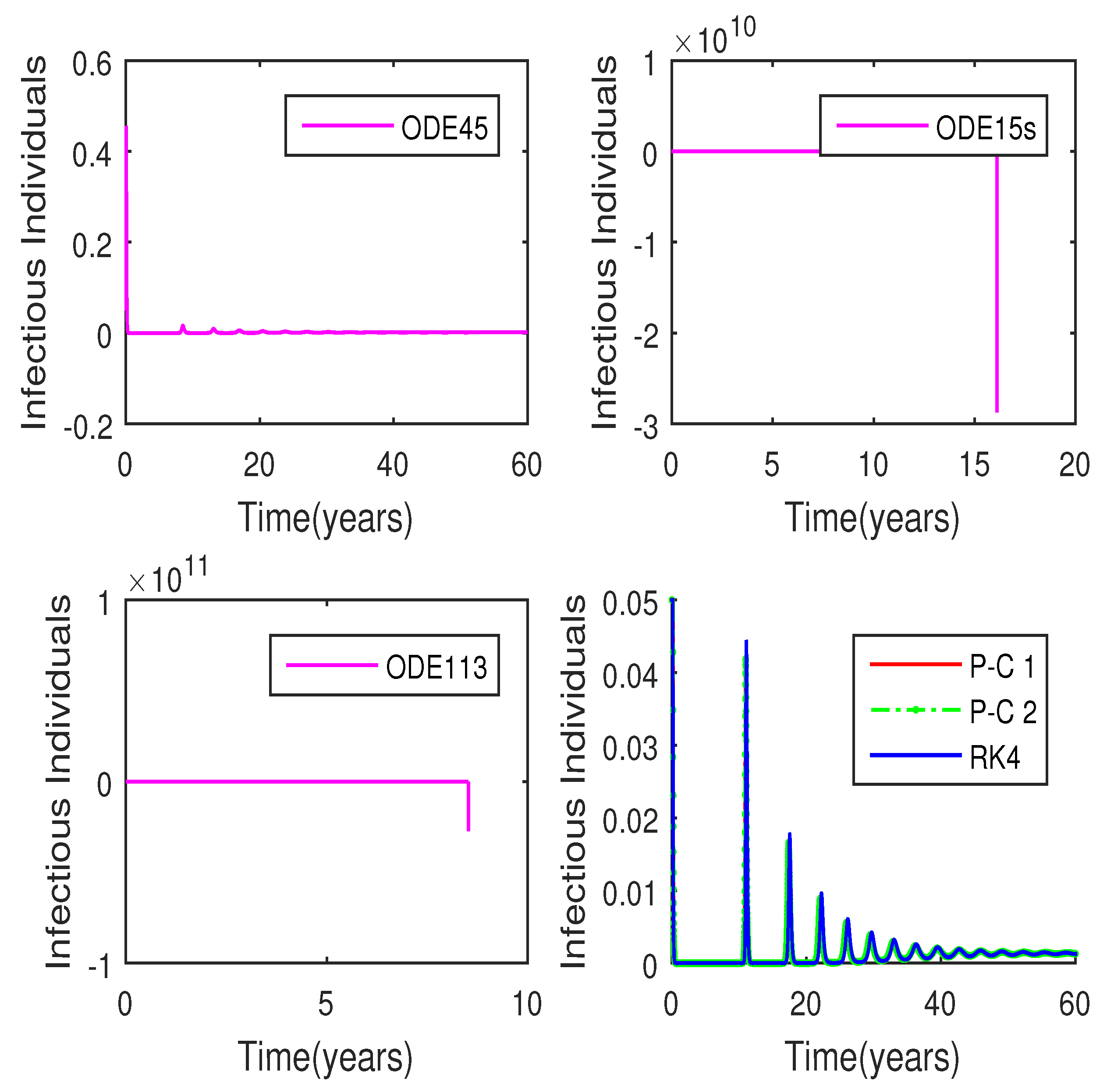
Abstract
:1. Introduction
2. The SIR Model
- is the coefficient of transmission;
- is the death rate or the birth rate, which are equal to each other;
- is the recovery rate;
- N is the total number of individuals, .
- (i)
- In the discrete derivatives of , and , a non-negative function substitutes the step size h, such that
- (ii)
- Nonlinear terms in the right hand side of (2) are approximated in a nonlocal way, that is to say, by an appropriate function of some points in the mesh.
3. Construction of New Schemes
3.1. Scheme 1
3.2. Scheme 2
4. Positivity
5. Elementary Stability
- ,
- ,
- .
6. The New Nonstandard Discretizations of SIR Model
- Step 1 Choose , and such that .
- Step 2 For do
- Step 3 Evaluate .
- Step 4 Via and , evaluate .
- Step 5 Correct the value , using , , .
- Step 6 Correct the value , using , , .
- Step 7 If and then
- Step 8 Calculate , else , and go to step 5.
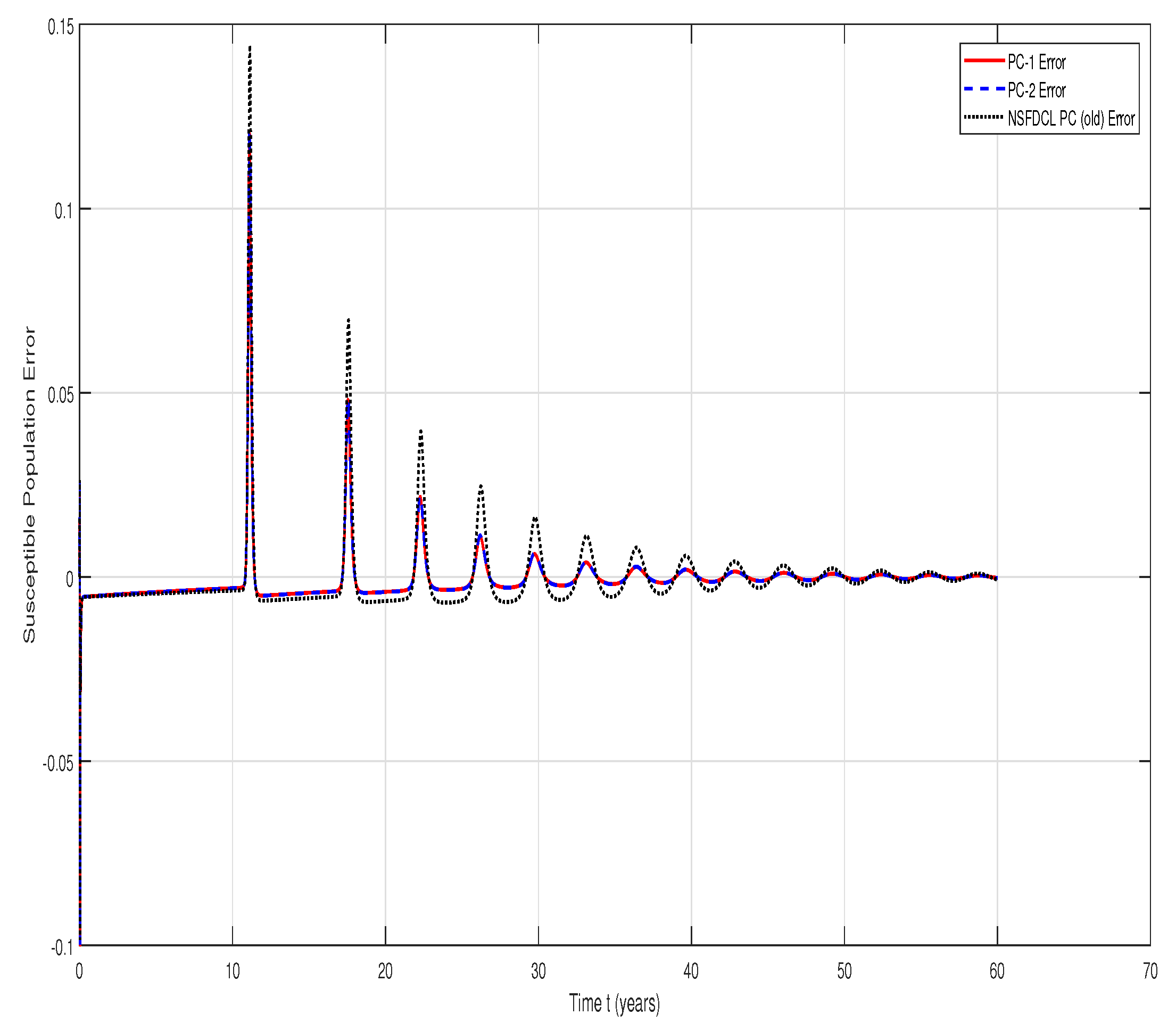
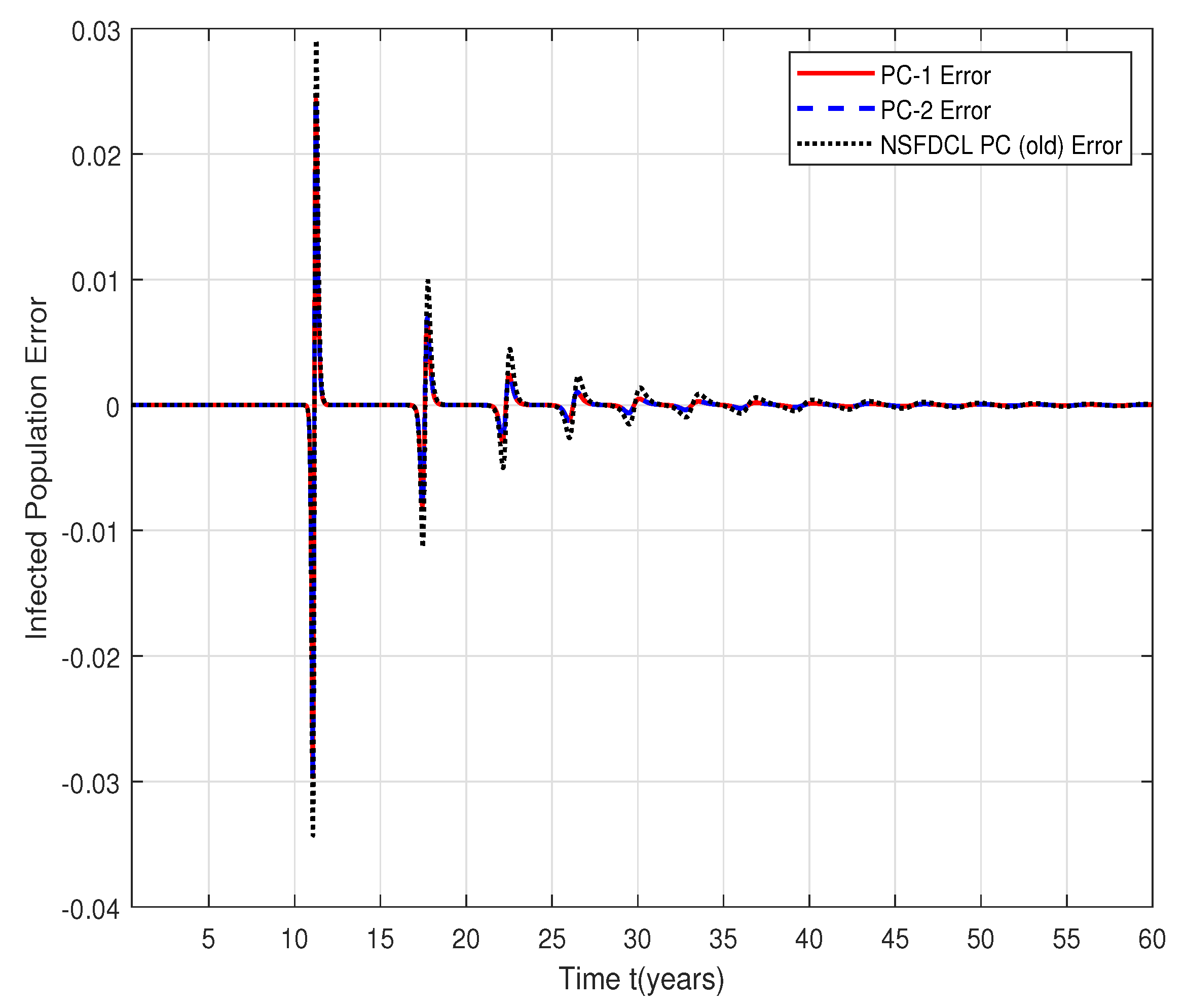
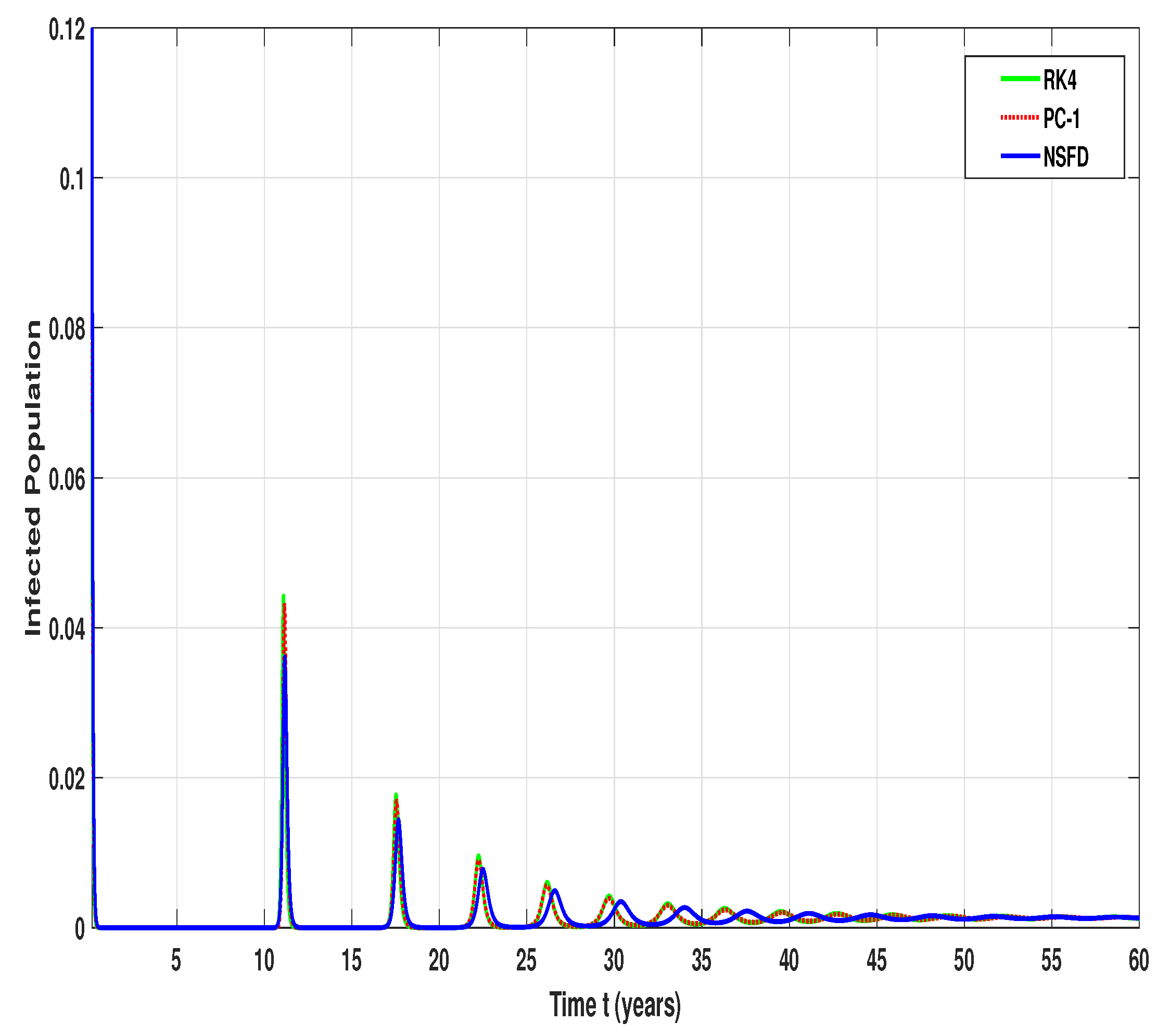
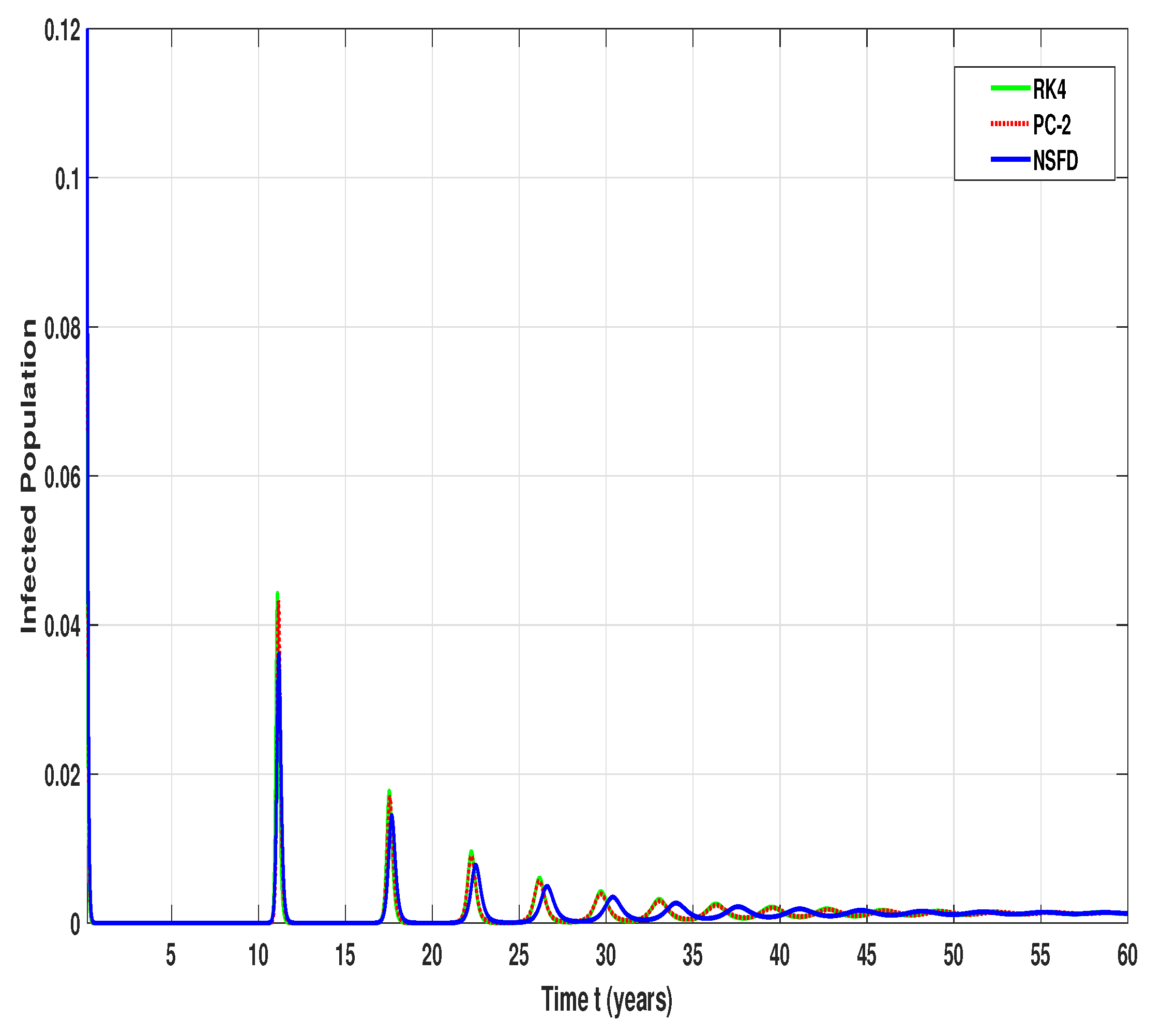
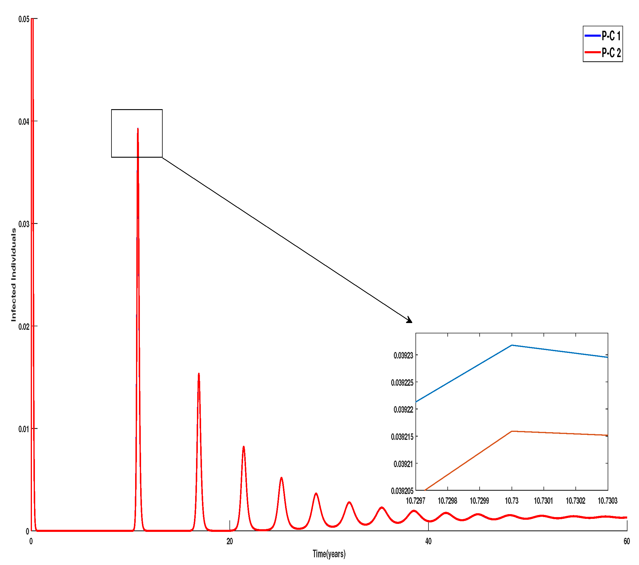
7. Numerical Results
8. Conclusions
Author Contributions
Funding
Institutional Review Board Statement
Informed Consent Statement
Data Availability Statement
Conflicts of Interest
References
- Ashyralyev, A.; Agirseven, D.; Agarwal, R.P. Stability estimates for delay parabolic differential and difference equations. Appl. Comput. Math. 2020, 19, 175–204. [Google Scholar]
- Ashyralyev, A.; Erdogan, A.S.; Tekalan, S.N. An investigation on finite difference method for the first order partial differential equation with the nonlocal boundary condition. Appl. Comput. Math. 2019, 18, 247–260. [Google Scholar]
- Odibat, Z. Fractional power series solutions of fractional differential equations by using generalized Taylor series. Appl. Comput. Math. 2020, 19, 47–58. [Google Scholar]
- Khalsaraei, M.M.; Shokri, A. The new classes of high order implicit six-step P-stable multiderivative methods for the numerical solution of schrödinger equation. Appl. Comput. Math. 2020, 19, 59–86. [Google Scholar]
- Khalsaraei, M.M.; Shokri, A. A new explicit singularly P-stable four-step method for the numerical solution of second order IVPs. Iranian J. Math. Chem. 2020, 11, 17–31. [Google Scholar]
- Ramos, H.; Popescu, P. How many k-step linear block methods exist and which of them is the most efficient and simplest one? Appl. Math. Comput. 2018, 316, 296–309. [Google Scholar] [CrossRef]
- Ramos, H.; Rufai, M.A. Numerical solution of boundary value problems by using an optimized two-step block method, Numer. Algorithms 2020, 84, 229–251. [Google Scholar] [CrossRef]
- Lambert, J.D. Computational Methods in Ordinary Differential Equations; Wiley: New York, NY, USA, 1973. [Google Scholar]
- Mickens, R.E. Nonstandard Finite Difference Models of Differential Equations; World Scientific: Singapore, 1994. [Google Scholar]
- Mickens, R.E. Nonstandard finite difference schemes for differential equations. J. Differ. Equations Appl. 2002, 8, 823–847. [Google Scholar] [CrossRef]
- Piyawong, W.; Twizell, E.H.; Gumel, A.B. An unconditionally convergent finite difference scheme for the SIR model. Appl. Math. Comput. 2003, 146, 611–625. [Google Scholar] [CrossRef]
- Ramos, H. Contributions to the development of differential systems exactly solved by multistep finite-difference schemes. Appl. Math. Comput. 2010, 217, 639–649. [Google Scholar] [CrossRef]
- Shokri, A.; Khalsaraei, M.M.; Molayi, M. Nonstandard Dynamically Consistent Numerical Methods for MSEIR Model. J. Appl. Comput. Mech. 2021, 8, 196–205. [Google Scholar]
- Shokri, A.; Khalsaraei, M.M.; Molayi, M. Dynamically Consistent NSFD Methods for Predator-prey System. J. Appl. Comput. Mech. 2021, 7, 1565–1574. [Google Scholar] [CrossRef]
- Anguelov, R.; Lubuma, J.M.S. Contributions to the mathematics of the nonstandard finite difference method and applications. Numer. Meth. Par. Diff. Eq. 2001, 17, 518–543. [Google Scholar] [CrossRef]
- Chen, C.; Wang, W.; Wang, X.; Wise, S.M. Positivity-preserving, energy stable numerical schemes for the Cahn-Hilliard equation with logarithmic potential. J. Comput. Phys. 2019, X3, 100031. [Google Scholar] [CrossRef]
- Dong, L.; Wang, C.; Zhang, H.A.; Zhang, Z. A positivity-preserving, energy stable and convergent numerical scheme for the cahn-hilliard equation with a flory-huggins-degennes energy. Commun. Math. Sci. 2019, 17, 921–939. [Google Scholar] [CrossRef]
- Iskenderov, N.S.; Allahverdiyeva, S.I. An inverse boundary value problem for the boussinesq-love equation with nonlocal integral condition. TWMS J. Pure Appl. Math. 2020, 11, 226–237. [Google Scholar]
- Qalandarov, A.A.; Khaldjigitov, A.A. Mathematical and numerical modeling of the coupled dynamic thermoelastic problems for isotropic bodies. TWMS J. Pure Appl. Math. 2020, 11, 119–126. [Google Scholar]
- Hale, J.K. Ordinary Differential Equations; Wiley-Interscience: New York, NY, USA, 1969. [Google Scholar]
- Roeger, L.W.; Barnard, R.W. Preservation of local dynamics when applying central difference methods: Application to SIR model. J. Differ. Equations Appl. 2007, 13, 333. [Google Scholar] [CrossRef]
- Khalsaraei, M.M.; Shokri, A.; Ramos, H.; Heydari, S. A positive and elementary stable nonstandard explicit scheme for a mathematical model of the influenza disease. Math. Comput. Simul. 2021, 182, 397–410. [Google Scholar] [CrossRef]
- Duncan, C.J.; Duncan, S.R.; Scott, S. Whooping cough epidemic in London, 1701–1812: Infection dynamics seasonal forcing and the effects of malnutrition. Proc. R. Soc. Lond. B 1996, 263, 445–450. [Google Scholar]
- Hethcote, H.W. The Mathematics of Infectious Diseases. SIAM Rev. 2000, 42, 599–653. [Google Scholar] [CrossRef]
- Mickens, R.E.; Jordan, P.M. A positivity-preserving nonstandard finite difference scheme for the Damped Wave Equation. Numer. Meth. Partial Diff. Eq. 2004, 20, 639–649. [Google Scholar] [CrossRef]
- Bacaer, N.; Ouifki, R.; Pretorius, C.; Wood, R.; Williams, B. Modeling the joint epidemics of TB and HIV in a south African township. J. Math. Biol. 2008, 57, 557–593. [Google Scholar] [CrossRef] [PubMed]
- Brauer, F.; Castillo-Chavez, C. Mathematical Models in Population Biology and Epidemiology; Texts in Applied Mathematics; Springer: New York, NY, USA, 2012; Volume 40. [Google Scholar] [CrossRef]
- Arenasa, A.J.; González-Parrab, G.; Chen-Charpentier, B.M. A nonstandard numerical scheme of predictor—Corrector type for epidemic models. Comput. Math. Appl. 2010, 59, 3740–3749. [Google Scholar] [CrossRef] [Green Version]


Publisher’s Note: MDPI stays neutral with regard to jurisdictional claims in published maps and institutional affiliations. |
© 2022 by the authors. Licensee MDPI, Basel, Switzerland. This article is an open access article distributed under the terms and conditions of the Creative Commons Attribution (CC BY) license (https://creativecommons.org/licenses/by/4.0/).
Share and Cite
Mehdizadeh Khalsaraei, M.; Shokri, A.; Ramos, H.; Yao, S.-W.; Molayi, M. Efficient Numerical Solutions to a SIR Epidemic Model. Mathematics 2022, 10, 3299. https://doi.org/10.3390/math10183299
Mehdizadeh Khalsaraei M, Shokri A, Ramos H, Yao S-W, Molayi M. Efficient Numerical Solutions to a SIR Epidemic Model. Mathematics. 2022; 10(18):3299. https://doi.org/10.3390/math10183299
Chicago/Turabian StyleMehdizadeh Khalsaraei, Mohammad, Ali Shokri, Higinio Ramos, Shao-Wen Yao, and Maryam Molayi. 2022. "Efficient Numerical Solutions to a SIR Epidemic Model" Mathematics 10, no. 18: 3299. https://doi.org/10.3390/math10183299