A New Regression Model on the Unit Interval: Properties, Estimation, and Application

Abstract

A new and flexible distribution is introduced for modeling proportional data based on the quantile of the generalized extreme value distribution. We obtain explicit expressions for the moments, quantiles, and other structural properties. An extended regression model is constructed as an alternative to compete with the beta regression. Some simulations from the Bayesian perspectives are developed, and an illustrative application to real data involving the comparison of models and influence diagnostics is also addressed.

1. Introduction

In recent years, we have seen a considerable interest in formulating new families of distributions for modeling proportional data: for example, illiteracy and mortality rates, the proportion of eggs hatched in the production of cuttings, percentage of defective items, etc. One of the most common distributions in this context is the beta distribution [1], which was also extended to a regression [2]. There are several extensions of the beta regression in Simas et al. [3], Ospina Ferrari [4], Ospina Ferrari [5], Carrasco et al. [6], and Figueroa-Zúñiga et al. [7].

Some other alternatives have appeared in the literature. For example, Qiu et al. [8] defined a simplex regression [9], Bayes et al. [10] introduced a parametric quantile regression from the Kumaraswamy distribution [11], Lemonte and Bazán [12] proposed a regression based on an extended Johnson $S_B$ distribution [13,14] introduced a family by compounding the cumulative distribution function (cdf) of a model with the quantile function (qf) of a second one. Cancho et al. [15] constructed a regression model by extending the Johnson $S_B$ distribution with a shape parameter controlling the asymmetry.

Let $F_X\left(x\right)$ be the baseline cdf of a random variable (rv) X with real support $\mathbb{R}$, and the transformation:

$$Y=G\left(\frac{X-\gamma }{\delta }\right),$$

(1)

where $G(·)$ is a cdf of an rv with support $\mathbb{R}$, $\gamma \in \mathbb{R}$, and $\delta >0$. Then, $X=\gamma +\delta Q\left(Y\right)$ for $y\in (0,1)$, where $Q\left(y\right)=G^{-1}\left(Y\right)$. The probability density function (pdf) of Y follows from (1) as:

$$f_Y\left(y\right)=\delta f_X(\gamma +\delta Q\left(y\right))\left|\frac{dQ\left(y\right)}{dy}\right|,$$

(2)

where $f_X\left(x\right)=d{F}_X\left(x\right)/dx$.

Let $X\sim N(0,1)$ have the standard normal cdf $\Phi \left(x\right)$, and $G\left(y\right)=1/(1+{\mathrm{e}}^{-y})$ the standard logistic cdf. Thus, the Johnson $S_B$ density follows from (2), for $y\in (0,1)$,

$$f_Y(y;\gamma ,\delta )=\frac{\delta \varphi (\gamma +\delta Q(y\left)\right)}{y(1-y)},$$

(3)

where $\varphi (·)$ is the standard normal density, and:

$$Q\left(y\right)=log\left(\frac{y}{1-y}\right),$$

(4)

is the logistic qf [14].

We define a new family by compounding a baseline standard normal with the qf of the generalized extreme value (GEV). Let Z be an rv having a GEV distribution [16] having cdf with zero location and unit scale parameter, namely:

$$G(z;\lambda )=\left\{\begin{array}{cc}exp\left[-{\left(1+\lambda z\right)}^{-1/\lambda }\right],\hfill & \hfill \lambda \ne 0;\\ exp\left(-{\mathrm{e}}^{-z}\right),\hfill & \hfill \lambda =0;\end{array}\right.$$

(5)

where $z\in [-1/\lambda ,+\infty )$ for $\lambda >0$, $z\in (-\infty ,-1/\lambda ]$ for $\lambda <0$ and $z\in (-\infty ,+\infty )$ for $\lambda =0$.

The qf of Z becomes:

$$Q(y;\lambda )=\left\{\begin{array}{cc}\frac{{[-log\left(y\right)]}^{-\lambda }-1}{\lambda },\hfill & \hfill \lambda >0\mathrm{and}y\in [0,1);\lambda <0\mathrm{and}y\in (0,1];\\ -log[-log(y\left)\right],\hfill & \hfill \lambda =0\mathrm{and}y\in (0,1).\end{array}\right.$$

(6)

This article is organized in six sections. Section 2 defines a new model called the normal-generalized extreme value (Normal-GEV) distribution, and provides some of its structural properties. Section 3 constructs a new regression model from this distribution, and addresses Bayesian inferential procedures. Section 4 performs several simulations under different scenarios to study the behavior of the estimators. An application to colorectal cancer data in Section 5 shows the importance of the proposed regression. Some conclusions are given in Section 6.

2. The Normal-GEV Distribution

The pdf of the rv $Y\sim \mathrm{Normal}-\mathrm{GEV}(\gamma ,\delta ,\lambda )$ follows by inserting (6) in Equation (3):

$$f_Y(y;\gamma ,\delta ,\lambda )=\frac{\delta \varphi \left(\gamma +\delta Q(y;\lambda )\right)}{y{\left[-\log \left(y\right)\right]}^{\lambda +1}},y\in (0,1).$$

(7)

Note that the above pdf includes both cases of Equation (6), i.e., the cases for $\lambda \ne 0$ and $\lambda \to 0$.

Proposition 1.

The limits below hold:

$$\underset{y\to 0^{+}}{lim}{f}_Y(y;\gamma ,\delta ,\lambda )=\left\{\begin{array}{cc}0,\hfill & \lambda <0;\hfill \\ \infty ,\hfill & \lambda ⩾0;\hfill \end{array}\right.and\underset{y\to 1^{-}}{lim}{f}_Y(y;\gamma ,\delta ,\lambda )=\left\{\begin{array}{cc}\delta \varphi (\gamma +\delta ),\hfill & \lambda =-1;\hfill \\ 0,\hfill & \lambda \ne -1.\hfill \end{array}\right.$$

Proof. 

Setting $x=-log\left(y\right)$, the Normal-GEV pdf (7) can be expressed as:

$$\begin{array}{c}\hfill f_Y(y;\gamma ,\delta ,\lambda )=\frac{\delta }{\sqrt{2\pi }}\left\{\begin{array}{cc}\frac{exp\left\{-\frac{1}{2}{\left[\gamma +\frac{\delta }{\lambda }(x^{-\lambda }-1)\right]}^2\right\}}{exp(-x)x^{\lambda +1}},\hfill & \lambda \ne 0;\hfill \\ \frac{exp\left\{-\frac{1}{2}{\left[\gamma +\delta (-log(x\left)\right)\right]}^2\right\}}{exp(-x)x},\hfill & \lambda =0.\hfill \end{array}\right.\end{array}$$

(8)

By using the known inequality:

$$\begin{array}{c}\hfill exp\left(x\right)⩾1+x,x\in \mathbb{R},\end{array}$$

(9)

the expression on the right-hand side of (8) reduces to:

$$\begin{array}{c}\hfill ⩾\frac{\delta }{\sqrt{2\pi }}\left\{\begin{array}{cc}\frac{1-\frac{1}{2}{\left[\gamma +\frac{\delta }{\lambda }(x^{-\lambda }-1)\right]}^2}{exp(-x)x^{\lambda +1}},\hfill & \lambda \ne 0;\hfill \\ \frac{1-\frac{1}{2}{\left[\gamma +\delta (-log(x\left)\right)\right]}^2}{exp(-x)x},\hfill & \lambda =0;\hfill \end{array}\right.=g(x;\gamma ,\delta ,\lambda ).\end{array}$$

That is, $f_Y(y;\gamma ,\delta ,\lambda )⩾g(x;\gamma ,\delta ,\lambda )$. We have ${lim}_{x\to \infty }g(x;\gamma ,\delta ,\lambda )=\infty$, $\forall \lambda ⩾0$, since the exponential grows faster than the polynomial. Then, since $y\to 0^{+}$⟺$x\to \infty$ from the squeeze (or sandwich) theorem, we get $\infty ={lim}_{x\to \infty }g(x;\gamma ,\delta ,\lambda )⩽{lim}_{y\to 0^{+}}{f}_Y(y;\gamma ,\delta ,\lambda )$. This proves that ${lim}_{y\to 0^{+}}{f}_Y(y;\gamma ,\delta ,\lambda )=\infty$, $\forall \lambda ⩾0$.

Again, by using (8) and inequality (9), we have:

$$\begin{array}{c}\hfill f_Y(y;\gamma ,\delta ,\lambda )⩽\frac{\delta }{\sqrt{2\pi }}\left\{\begin{array}{cc}\left(\frac{1-x}{x^{\lambda +1}}\right)exp\left\{-\frac{1}{2}{\left[\gamma +\frac{\delta }{\lambda }(x^{-\lambda }-1)\right]}^2\right\},\hfill & \lambda \ne 0;\hfill \\ \left(\frac{1-x}{x}\right)exp\left\{-\frac{1}{2}{\left[\gamma +\delta (-log(x\left)\right)\right]}^2\right\},\hfill & \lambda =0;\hfill \end{array}\right.=h(x;\gamma ,\delta ,\lambda ).\end{array}$$

For $\lambda <0$, from the inequality above and by the rapid growth of the exponential in comparison to polynomials, we have ${lim}_{y\to 0^{+}}{f}_Y(y;\gamma ,\delta ,\lambda )⩽{lim}_{x\to \infty }h(x;\gamma ,\delta ,\lambda )=0$. Therefore, ${lim}_{y\to 0^{+}}{f}_Y(y;\gamma ,\delta ,\lambda )=0$, $\forall \lambda <0$.

On the other hand, note that $y\to 1^{-}$⟺$x\to 0$. Again, from the inequality $f_Y(y;\gamma ,\delta ,\lambda )⩽h(x;\gamma ,\delta ,\lambda )$ and the rapid growth of the exponential, $\forall \lambda \ne 1$, we get ${lim}_{y\to 1^{-}}{f}_Y(y;\gamma ,\delta ,\lambda )⩽{lim}_{x\to 0}h(x;\gamma ,\delta ,\lambda )=0$. Hence, ${lim}_{y\to 1^{-}}{f}_Y(y;\gamma ,\delta ,\lambda )=0$.

Finally, if $\lambda =-1$, then $f_Y$ in (7) gives:

$$f_Y(y;\gamma ,\delta ,-1)=\frac{\delta \varphi \left(\gamma +\delta [log(y)+1]\right)}{y},y\in (0,1).$$

Then, it is clear that (by the continuity of $\varphi$), ${lim}_{y\to 1^{-}}{f}_Y(y;\gamma ,\delta ,-1)=\delta \varphi (\gamma +\delta )$. □

The proof of the next result is immediate and hence omitted.

Proposition 2.

Let $Y\sim Normal-GEV(\gamma ,\delta ,\lambda )$, and $T_{\gamma ,\delta ,\lambda }\left(y\right)=\gamma +\delta Q(y;\lambda )$. The cdf of Y is

$$F_Y\left(y\right)=\Phi \left(T_{\gamma ,\delta ,\lambda }\left(y\right)\right),y\in (0,1),$$

where$Q(y;\lambda )$is as in (6).

2.1. Behavior of the Normal-GEV Distribution

In this subsection, some distributional properties such as unimodality and monotonicity of the Normal-GEV pdf are analyzed.

To determine the number of modes of a pdf, f, it is necessary to locate its critical points. By definition, a critical point of a function f is a point on the graph of f where the derivative is zero or infinite.

Proposition 3.

All critical points y of the new pdf (7) satisfy:

$$\begin{array}{c}\hfill [\lambda +1+log\left(y\right)]{[-log\left(y\right)]}^{\lambda }-\delta [\gamma +\delta Q(y;\lambda )]=0,\end{array}$$

where $Q(y;\lambda )$ is given in (6).

Proof. 

Adopting the notation of Proposition 2, $f_Y\left(y\right)=f_Y(y;\gamma ,\delta ,\lambda )$ and $T\left(y\right)=T_{\gamma ,\delta ,\lambda }\left(y\right)=\gamma +\delta Q(y;\lambda )$, we have (dashes mean derivatives) $f_Y\left(y\right)=\varphi \left(T\left(y\right)\right)T^{\prime }\left(y\right)$. Differentiating $f_Y\left(y\right)$ with respect to y gives:

$$\begin{array}{c}\hfill f_Y^{\prime }\left(y\right)=\varphi \left(T\left(y\right)\right)\left\{T^{″}\left(y\right)-T\left(y\right){\left[T^{\prime }\left(y\right)\right]}^2\right\},\end{array}$$

(10)

where:

$$\begin{array}{c}\hfill T^{\prime }\left(y\right)=\delta \frac{{[-log\left(y\right)]}^{-(\lambda +1)}}{y}\mathrm{and}{T}^{″}\left(y\right)=T^{\prime }\left(y\right)\frac{{[-log\left(y\right)]}^{-1}[\lambda +1+log\left(y\right)]}{y}.\end{array}$$

(11)

By combining (10) and (11), we obtain:

$$\begin{array}{c}\hfill f_Y^{\prime }\left(y\right)=\frac{f_Y\left(y\right){[-log\left(y\right)]}^{-(\lambda +1)}}{y}\left\{[\lambda +1+log\left(y\right)]{[-log\left(y\right)]}^{\lambda }-\delta [\gamma +\delta Q(y;\lambda )]\right\}.\end{array}$$

Then, the proof follows. □

Theorems 1 and 2 show that $\lambda$ governs the shape of the new distribution.

Theorem 1.

If$Y\sim Normal-GEV(\gamma ,\delta ,\lambda )$with$\lambda \ne 0$, the pdf of Y is:

• Decreasing-increasing-decreasing (DID) or decreasing (D) whenever$\lambda \in \mathbb{N}$.
• Unimodal whenever $\lambda \in \mathbb{Z}\backslash (\mathbb{N}\cup \{-1,0\left\}\right)$ and $\gamma <\delta /\lambda$.

Proof. 

By replacing $Q(y;\lambda )$ with $\lambda \ne 0$ in equation of Proposition 3, all critical points y of the pdf of Y satisfy:

$$\begin{array}{c}\hfill p\left(x\right)=-x^{2\lambda +1}+(\lambda +1)x^{2\lambda }+\delta \left(\frac{\delta }{\lambda }-\gamma \right)x^{\lambda }-\frac{{\delta }^2}{\lambda }=0,\mathrm{with}x=-log\left(y\right).\end{array}$$

If $\lambda \in \mathbb{N}$, then $p\left(x\right)$ is a polynomial of degree $2\lambda +1$. By Descartes’ rule of signs [17], $p\left(x\right)$ has two sign changes (regardless of the sign of $\delta /\lambda -\gamma$) and then two or zero positive roots. If $p\left(x\right)$ has two positive roots $x_1$ and $x_2$, the pdf of Y has two critical points $y_1=exp(-x_1)$ and $y_2=exp(-x_2)$ in $(0,1)$. On the other hand, if $p\left(x\right)$ has zero positive roots, it has no critical points in $(0,1)$. Finally, since ${lim}_{y\to 0^{+}}{f}_Y\left(y\right)=\infty$ and ${lim}_{y\to 1}{f}_Y\left(y\right)=0$, the statement of Item 1 follows.

If $\lambda \in \mathbb{Z}\backslash (\mathbb{N}\cup \{-1,0\left\}\right)$, $p\left(x\right)$ can be written in terms of $w=x^{-1}={[-log\left(y\right)]}^{-1}$

$$\begin{array}{c}\hfill q\left(w\right)=-w^{-2\lambda -1}+(\lambda +1)w^{-2\lambda }+\delta \left(\frac{\delta }{\lambda }-\gamma \right)w^{-\lambda }-\frac{{\delta }^2}{\lambda }=0.\end{array}$$

In this case, $q\left(w\right)$ is a polynomial of degree $-2\lambda -1$. Again, by Descartes’ rule of signs, $q\left(w\right)$ has only one sign change, and this polynomial has only one positive root, say $w_0$. Then, the pdf of Y has only one critical point $y_0=exp(-w_0^{-1})$ on $(0,1)$. Since ${lim}_{y\to 0^{+}}{f}_Y\left(y\right)=0$ and ${lim}_{y\to 1}{f}_Y\left(y\right)=\delta \varphi (\gamma +\delta ){\delta }_{\lambda ,-1}$, where ${\delta }_{i,j}$ is the Kronecker delta, the unimodality stated in Item 2 follows. □

Theorem 2 provides the explicit critical points of the Normal-GEV pdf ($\lambda =0$) whenever a constraint on parameters $\gamma$ and $\delta$ is imposed. Further, this theorem shows that the form of the pdf is continuous monotone at three disjoint intervals.

Theorem 2.

If $Y\sim Normal-GEV(\gamma ,\delta ,\lambda )$ and $\lambda =0$, the pdf of Y is decreasing-increasing-decreasing (DID) whenever:

$$\begin{array}{c}\hfill \gamma ⩽[2log\left(\delta \right)-1]\delta +\frac{1}{\delta }.\end{array}$$

(12)

Moreover,

$$y_1=exp\left[{\delta }^2{W}_{-1}\right(-\frac{exp(\frac{\gamma }{\delta }-\frac{1}{{\delta }^2})}{{\delta }^2}\left)\right]\mathrm{and}{y}_2=exp\left[{\delta }^2{W}_0\right(-\frac{exp(\frac{\gamma }{\delta }-\frac{1}{{\delta }^2})}{{\delta }^2}\left)\right]$$

(13)

are the minimum and maximum points of the pdf of Y, respectively. For some integer k, $W_k(·)$ denotes the Lambert W function.

Proof. 

By replacing the definition of $Q(y;\lambda )$ with $\lambda =0$ in the equation of Proposition 3, all critical points y of the pdf of Y satisfy:

$$\begin{array}{c}\hfill 1-x+{\delta }^{2}log\left(x\right)-\delta \gamma =0,\mathrm{with}x=-log\left(y\right).\end{array}$$

Equivalently,

$$\begin{array}{c}\hfill \left(-\frac{x}{{\delta }^2}\right)exp\left(-\frac{x}{{\delta }^2}\right)=-\frac{exp(\frac{\gamma }{\delta }-\frac{1}{{\delta }^2})}{{\delta }^2}.\end{array}$$

Since the function $f\left(t\right)=texp\left(t\right)$ has a (global) minimum $-1/\mathrm{e}$ at the point $t=-1$, the above equation can be solved for $-x/{\delta }^2$ only if $z=-exp(\frac{\gamma }{\delta }-\frac{1}{{\delta }^2})/{\delta }^2⩾-1/\mathrm{e}$. Since $z<0$, assuming the condition (12), the two values $y_1$ and $y_2$ in (13) are obtained. Finally, $y_1$ and $y_2$ are minimum and maximum points of the pdf of Y, respectively, because ${lim}_{y\to 0^{+}}{f}_Y\left(y\right)=\infty$ and ${lim}_{y\to 1}{f}_Y\left(y\right)=0$, and $0<y_1<y_2<1$. □

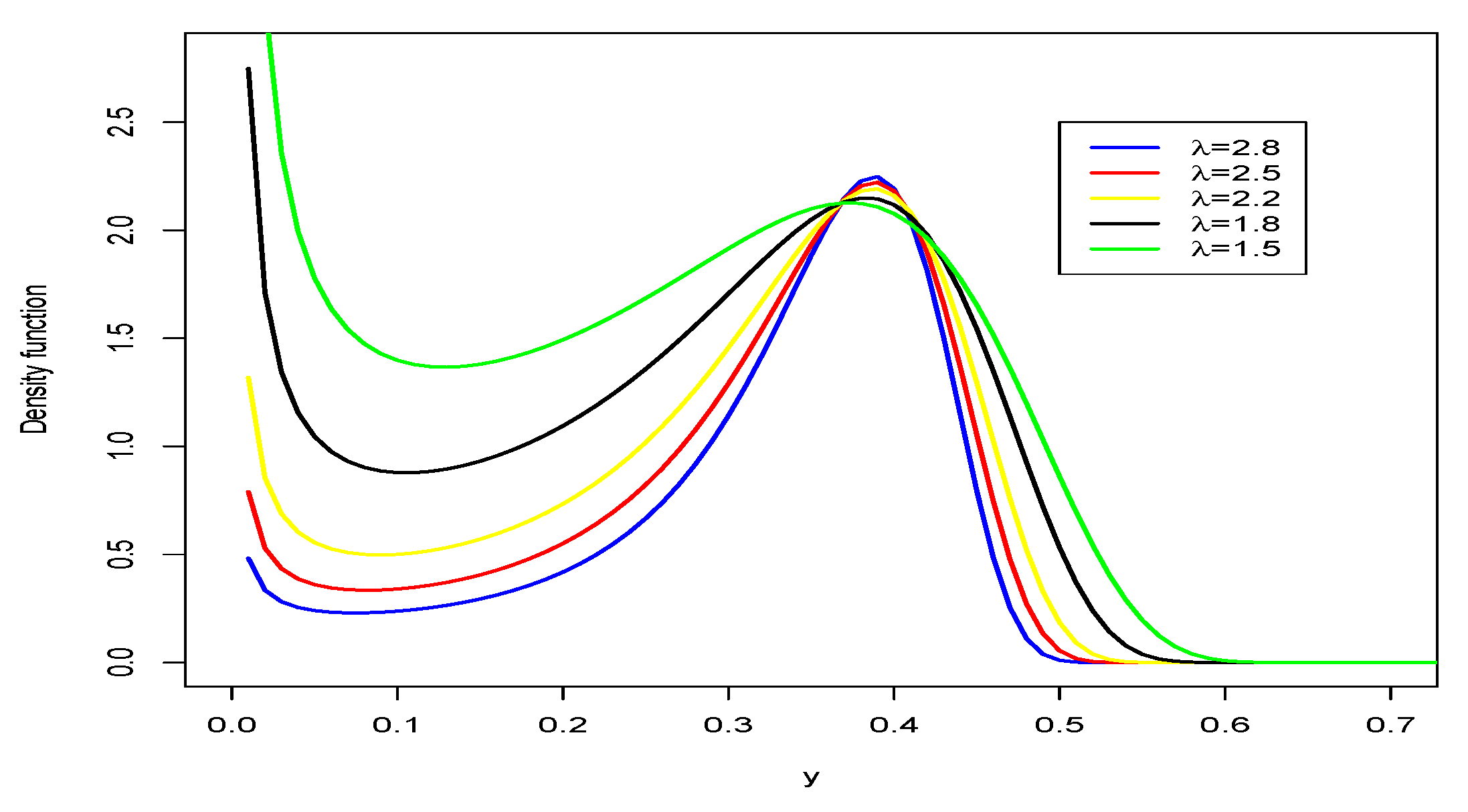
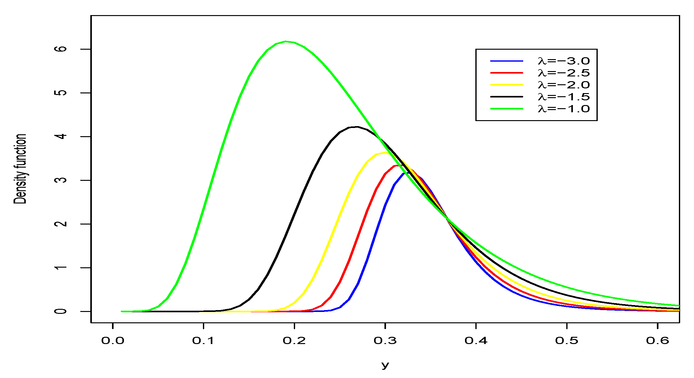
Figure 1 and Figure 2 reveal different types of asymmetrical. For negative values of the parameter $\lambda$ we have positive asymmetry (and unimodality), for positive values of $\lambda$ we have decreasing, increasing and decreasing behavior.

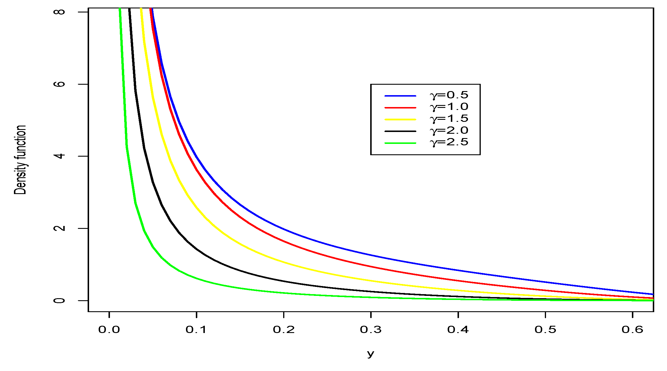
Figure 3 shows that cases of decreasing strict monotonicity can appear in the Normal-GEV pdf.

2.2. Related Distributions

Proposition 4.

If$Y\sim Normal-GEV(\gamma ,\delta ,\lambda )$, then (for any$a>0$and$b\in \mathbb{R}$):

• Normal distribution: $a\delta Q(Y;\lambda )+a\gamma +b\sim N(b,a^2)$.
• Log-normal distribution: $exp[a\delta Q(Y;\lambda )+a\gamma +b]\sim log\left[N(b,a^2)\right]$.
• Folded normal distribution: $|a\delta Q(Y;\lambda )+a\gamma +b|\sim N_f(b,a^2)$.
• χ distribution with one degree of freedom (df): $|a\delta Q(Y;\lambda )+a\gamma |/a\sim {\chi }_1$.
• Noncentral ${\chi }^2$ distribution: ${[a\delta Q(Y;\lambda )+a\gamma +b]}^2/a^2\sim {\chi }_1^2(b^2/a^2)$.
• Lévy distribution: ${[a\delta Q(Y;\lambda )+a\gamma ]}^{-2}\sim \mathrm{Levy}(0,a^{-2})$.

Proof. 

The proof of this proposition follows by using well-known properties of the normal distribution with Equation (1). Hence, details are omitted. □

Proposition 5.

• ${\chi }^2$distribution with n df: If$Y_k\sim Normal-GEV({\gamma }_k,{\delta }_k,{\lambda }_k)$, $k=1,\dots ,n$, are independent rvs, then:

  $$\begin{array}{c}\hfill {[{\delta }_{1}Q(Y_1;{\lambda }_1)+{\gamma }_1]}^2+\cdots +{[{\delta }_{n}Q(Y_n;{\lambda }_n)+{\gamma }_n]}^2\sim {\chi }_n^2.\end{array}$$
• Student t-distribution with$n-1$df: If$Y_k\sim Normal-GEV({\gamma }_k,{\delta }_k,{\lambda }_k)$, $k=1,\dots ,n$, are independent rvs, then:

  $$\begin{array}{c}\hfill \frac{\overline{X}}{\sqrt{\frac{1}{n(n-1)}[{({\delta }_{1}Q(Y_1;{\lambda }_1)+{\gamma }_1-\overline{X})}^2+\cdots +{({\delta }_{n}Q(Y_n;{\lambda }_n)+{\gamma }_n-\overline{X})}^2]}}\sim t_{n-1},\end{array}$$

  where$\overline{X}=\{[{\delta }_{1}Q(Y_1;{\lambda }_1)+\cdots +{\delta }_{n}Q(Y_n;{\lambda }_n)]+({\gamma }_1+\cdots +{\gamma }_n)\}/n$.
• F-distribution with$(n,m)$df: If$Y_k\sim Normal-GEV({\gamma }_k,{\delta }_k,{\lambda }_k)$, $k=1,\dots ,n$, $Y_j^{\prime }\sim Normal-GEV({\gamma }_j^{\prime },{\delta }_j^{\prime },{\lambda }_j^{\prime })$, $j=1,\dots ,m$, are independent rvs, then:

  $$\begin{array}{c}\hfill \frac{\{{[{\delta }_{1}Q(Y_1;{\lambda }_1)+{\gamma }_1]}^2+\cdots +{[{\delta }_{n}Q(Y_n;{\lambda }_n)+{\gamma }_n]}^2\}/n}{\{{[{\delta }_1^{\prime }Q(Y_1^{\prime };{\lambda }_1^{\prime })+{\gamma }_1^{\prime }]}^2+\cdots +{[{\delta }_m^{\prime }Q(Y_m^{\prime };{\lambda }_m^{\prime })+{\gamma }_m^{\prime }]}^2\}/m}\sim F_{n,m}.\end{array}$$

Proof. 

The proof follows by combining known properties of the normal distribution with Equation (1). □

2.3. The New Model as a Limit Distribution

Let $\overline{X}$ be the sample mean of n samples drawn from a population with mean $\mu$ and standard deviation $\sigma \in (0,\infty )$. The central limit theorem leads to the well-known result:

$$\begin{array}{c}\hfill \frac{\overline{X}-\mu }{\sigma /\sqrt{n}}\stackrel{\mathcal{D}}{⟶}Z\sim N(0,1),\end{array}$$

where “$\stackrel{\mathcal{D}}{⟶}$” denotes convergence in the distribution. Let $T_{\gamma ,\delta ,\lambda }$ be the transformation defined in Proposition 2. Since $T_{\gamma ,\delta ,\lambda }^{-1}$ is a continuous map, by applying the continuous mapping theorem, we have:

$$\begin{array}{c}\hfill T_{\gamma ,\delta ,\lambda }^{-1}\left(\frac{\overline{X}-\mu }{\sigma /\sqrt{n}}\right)\stackrel{\mathcal{D}}{⟶}Y:=T_{\gamma ,\delta ,\lambda }^{-1}\left(Z\right).\end{array}$$

From Equation (1), $Y=T_{\gamma ,\delta ,\lambda }^{-1}\left(Z\right)\sim \mathrm{Normal}-\mathrm{GEV}(\gamma ,\delta ,\lambda )$, where $T_{\gamma ,\delta ,\lambda }^{-1}\left(z\right)=G((z-\gamma )/\delta ;\lambda )$ and $G(·)$ is the GEV cdf given in (5).

Then, for $\lambda \ne 0$:

$$\begin{array}{c}\hfill exp\left[-{\left(1+\frac{\lambda }{\delta }\left(\frac{\overline{X}-\mu }{\sigma /\sqrt{n}}-\gamma \right)\right)}^{-1/\lambda }\right]\stackrel{\mathcal{D}}{⟶}Y\sim \mathrm{Normal}-\mathrm{GEV}(\gamma ,\delta ,\lambda );\end{array}$$

and, for $\lambda =0$,

$$\begin{array}{c}\hfill exp\left[-\exp \left(-\frac{1}{\delta }\left(\frac{\overline{X}-\mu }{\sigma /\sqrt{n}}-\gamma \right)\right)\right]\stackrel{\mathcal{D}}{⟶}Y\sim \mathrm{Normal}-\mathrm{GEV}(\gamma ,\delta ,0).\end{array}$$

2.4. Moments, Quantile and Other Measures

Proposition 6.

The rth real moment of $Y\sim Normal-GEV(\gamma ,\delta ,\lambda )$ is (whenever it makes sense):

$$E\left[Y^r\right]=M_{{\phi }_{\lambda }\left(Z\right)}\left(r\right),Z\sim N(0,1),$$

(14)

where,

$$\begin{array}{c}\hfill {\phi }_{\lambda }\left(z\right)=\left\{\begin{array}{cc}-{(1-\frac{\lambda \gamma }{\delta }+\frac{\lambda }{\delta }z)}^{-1/\lambda },\hfill & \mathrm{if}\lambda \ne 0;\hfill \\ -exp\left(\frac{\gamma -z}{\delta }\right),\hfill & \mathrm{if}\lambda =0,\hfill \end{array}\right.\end{array}$$

and $M_X(·)$ is the generating function of X. For example, for $\lambda =-1$, $E\left[Y^r\right]=exp(\frac{\lambda \gamma }{\delta }+\frac{r^2{\lambda }^2}{2{\delta }^2}-1)$.

Proof. 

The proof is immediate since Y follows Equation (1) with $G(·)$ given in (5). □

The moments of Y are finite since its support is limited, and the integral in (14) can be numerically computed via the software R, Mathematica, and Maple, among others. Specifically, the mean and variance are calculated using the integrate function of the R software. This approximation is based on the adaptive quadrature of functions of one variable over a finite interval; for more details, see Piessens et al. [18].

Table 1. Mean and variance of the Normal-GEV distribution.

Parameter	Mean	Variance	Parameter	Mean	Variance	Parameter	Mean	Variance
$\lambda =0.5$			$\lambda =0.1$			$\lambda =0.5$
$\gamma =0.2$	0.3212	0.0279	$\gamma =2$	0.0921	0.0100	$\gamma =0.2$	0.3047	0.0622
$\delta =2$			$\delta =2$			$\delta =1$
$\lambda =0.1$			$\lambda =0.1$			$\lambda =0.5$
$\gamma =0.2$	0.3341	0.0266	$\gamma =1$	0.2105	0.0213	$\gamma =0.2$	0.3212	0.0279
$\delta =2$			$\delta =2$			$\delta =2$
$\lambda =0$			$\lambda =0.1$			$\lambda =0.5$
$\gamma =0.2$	0.3373	0.0265	$\gamma =0.5$	0.2856	0.0254	$\gamma =0.2$	0.3359	0.0144
$\delta =2$			$\delta =2$			$\delta =3$
$\lambda =-0.2$			$\lambda =0.1$			$\lambda =0.5$
$\gamma =0.2$	0.3437	0.0267	$\gamma =0.2$	0.3341	0.0266	$\gamma =0.2$	0.3532	0.0038
$\delta =2$			$\delta =2$			$\delta =6$
$\lambda =-0.5$			$\lambda =0.1$			$\lambda =0.5$
$\gamma =0.2$	0.3538	0.0281	$\gamma =0$	0.3666	0.0269	$\gamma =0.2$	0.3573	0.0021
$\delta =2$			$\delta =2$			$\delta =8$

reports the mean and variance of Y for some parameters obtained numerically using the integrate function of the R software. We note in the second and third columns that the mean and variance do not change for different values of $\lambda$. However, there is some variation of the variance for different values of $\gamma$ with the other parameters fixed. So, the parameter $\gamma$ is responsible for the location of the model and the parameter $\delta$ for the dispersion.

Proposition 7.

Let $Y\sim Normal-GEV(\gamma ,\delta ,\lambda )$. Then, the qth quantile of Y is:

$$y_q=\left\{\begin{array}{cc}exp\left\{-{[1+\frac{\lambda }{\delta }(x_q-\gamma )]}^{-\frac{1}{\lambda }}\right\},\hfill & \hfill \lambda \ne 0;\\ exp\left\{-exp\left[-\left(\frac{x_q-\gamma }{\delta }\right)\right]\right\},\hfill & \hfill \lambda =0,\end{array}\right.$$

where $x_q$ is the qth standard normal quantile (for $0<q<1$).

Proof. 

The proof is immediate and then omitted. □

The median $\nu$ of the Normal-GEV distribution follows from Proposition 7:

$$\nu =\left\{\begin{array}{cc}exp\left\{-{\left(1+\frac{\lambda }{\delta }(-\gamma )\right)}^{-\frac{1}{\lambda }}\right\},\hfill & \hfill \lambda \ne 0;\\ exp\left\{-\exp \left(\frac{-\gamma }{\delta }\right)\right\},\hfill & \hfill \lambda =0;\end{array}\right.$$

(15)

where $x_{0.5}$ is the median of the standard normal distribution. Furthermore, from Proposition 7, the random values for Y can be easily generated.

Further, the Bowley’s skewness of Y is:

$$B=\frac{y_{0.75}+y_{0.25}-2\nu }{y_{0.75}-y_{0.25}},$$

where $y_{0.25},\nu$ and $y_{0.75}$ are the quantile values.

Figure 4 displays the skewness of Y for some parameters, which indicates that the distribution is symmetric when $\lambda ⟶0$ and $\gamma ⟶0$. Thus, the parameters $\lambda$ and $\gamma$ govern the skewness of Y.

3. Bayesian Inference for the Normal-GEV Regression

The Normal-GEV median can be expressed from (15) as:

$$\gamma =-\delta Q(\nu ;\lambda ),$$

where $Q(y;\lambda )$ is given by (6). Therefore, it has a simple form to construct a regression model. In this context, we obtain a reparameterized density of Y by replacing the above expression in Equation (2),

$$f(y;\lambda ,\nu ,\delta )=\frac{\delta \varphi \left(\delta \left[Q\right(y;\lambda )-Q(\nu ;\lambda \left)\right]\right)}{y{[-\log \left(y\right)]}^{\lambda +1}},y\in (0,1),$$

(16)

where $\lambda \in \mathbb{R}$, $\nu \in (0,1)$, and $\delta >0$ works as a dispersion parameter.

Let $\mathbf{y}={(y_1,\cdots ,y_n)}^{\top }$ be n observations from $Y_i\sim \mathrm{Normal}-\mathrm{GEV}(\lambda ,{\nu }_i,{\delta }_i)$, where two systematic components are constructed for the median ${\nu }_i$ and dispersion ${\delta }_i$. The Normal-GEV regression model is defined by (16) and the systematic components:

$${\eta }_{1i}=h_1\left({\nu }_i\right)={\mathbf{w}}_i^{\top }\beta \mathrm{and}{\eta }_{2i}=h_2\left({\delta }_i\right)={\mathbf{z}}_i^{\top }\tau ,$$

where ${\mathbf{w}}_i={(w_{1i},\cdots ,w_{pi})}^{\top }$ and ${\mathbf{z}}_i={(z_{1i},\cdots ,z_{qi})}^{\top }$ are vectors of covariates, $\beta \in {\mathbb{R}}^p$, $\tau \in {\mathbb{R}}^q$ are vectors of unknown coefficients ($p+q<n$), and $h_1:(0,1)⟶\mathbb{R}$ and $h_2:(0,\infty )⟶\mathbb{R}$ are strictly monotonic and twice differentiable link functions. There are several possible choice for the link functions $h_1$ and $h_2$. For example, some useful link functions for the median are: logit $h_1\left(\nu \right)=\log \left(\frac{\nu }{1-\nu }\right)$; probit $h_1\left(\nu \right)={\Phi }^{-1}\left(\nu \right)$, where ${\Phi }^{-1}(·)$ is the standard normal quantile function; complementary log–log$h_1\left(\nu \right)=\log \left[-\log (1-\nu )\right]$; log–log $h_1\left(\nu \right)=-\log \left[-\log \left(\nu \right)\right]$; and Cauchy $h_1\left(\psi \right)=\tan \left[\pi (\psi -0.5)\right]$. Some possible choice dispersion link are: logarithmic $h_2\left(\delta \right)=\log \left(\delta \right)$; square root $h_2\left(\delta \right)=\sqrt{\delta }$; identity $h_2\left(\delta \right)=\delta$ (with $\delta >0$); among others. The relationship between $\nu$ and $\mathbf{\beta }$ and ${\delta }_i$ and $\mathbf{\tau }$ is equivalent to a canonical link for ${\nu }_i$ ( location parameter) and ${\delta }_i$ (dispersion parameter) in setting generalized linear model.

Further, let $\mathit{W}={(w_1,\cdots ,w_n)}^{\top }$ and $\mathit{Z}={(z_1,\cdots ,z_n)}^{\top }$ be matrices of full ranks p and q, respectively. The likelihood function for the parameters given the observed data $\mathcal{D}=(y,\mathit{W},\mathit{Z})$ has the form:

$$L(\lambda ,\mathbf{\beta },\mathbf{\tau }|\mathcal{D})=\prod _{i=1}^n{\delta }_i\varphi \left({\delta }_i[Q(y_i;\lambda )-Q({\nu }_i;\lambda )]\right){\left[\prod _{i=1}^n{y}_i\right]}^{-1}{\left[\prod _{i=1}^n{(-\log \left(y_i\right))}^{\lambda +1}\right]}^{-1}.$$

(17)

Maximizing (17) provides the maximum likelihood estimates (MLEs) of the parameters. However, we consider the Bayesian method with the common proper prior distributions:

$$\begin{array}{c}\hfill {\beta }_j\sim \mathrm{Nl}(0,100),j=1,\dots ,p,{\tau }_j\sim \mathrm{N}(0,100),j=1,\dots q,\mathrm{and}\lambda \sim \mathrm{N}(0,1),\end{array}$$

(18)

where $\mathbf{\beta }$, $\mathbf{\tau }$, and $\lambda$ are assumed independent. Combining (17) and (18), the joint posterior density for $\mathbf{\vartheta }=(\lambda ,\mathbf{\beta },\mathbf{\tau })\in {\mathbb{R}}^{p+q+1}$ reduces to:

$$\begin{array}{cc}\hfill \pi \left(\mathbf{\vartheta }\right|\mathcal{D})& \propto \prod _{i=1}^n{\delta }_i\varphi \left({\delta }_i[Q(y_i;\lambda )-Q({\nu }_i;\lambda )]\right){\left[\prod _{i=1}^n{(-\log \left(y_i\right))}^{\lambda +1}\right]}^{-1}\pi \left(\lambda \right)\pi \left(\mathbf{\beta }\right)\pi \left(\mathbf{\tau }\right).\hfill \end{array}$$

The Metropolis–Hastings algorithm consists of the steps:

(1)

Initialize from trial ${\mathbf{\vartheta }}_{\left(0\right)}$ and set $j=0$;

(2)

Construct the transitional kernel $K({\mathbf{\vartheta }}^{\prime },{\mathbf{\vartheta }}_j)=N_{p+q+1}\left({\mathbf{\vartheta }}_j,\tilde{\Sigma }\right)$ to generate a new point ${\mathbf{\vartheta }}^{\prime }$, where $\tilde{\Sigma }$ is evaluated at ${\mathbf{\vartheta }}_j$;

(3)

Update ${\mathbf{\vartheta }}_{\left(j\right)}$ to ${\mathbf{\vartheta }}_{(j+1)}={\mathbf{\vartheta }}^{\prime }$ with probability $p_j=min\{1,\pi \left({\mathbf{\vartheta }}^{\prime }\right|\mathcal{D})/\pi \left({\mathbf{\vartheta }}_{\left(j\right)}\right|\mathcal{D})\}$, or set ${\mathbf{\vartheta }}_{\left(j\right)}$ with probability $1-p_j$;

(4)

Steps (2) and (3) are repeated until the process becomes stationary.

The script can be obtained from the authors upon request. For more details on the Metropolis–Hastings algorithm, we refer to Chib et al. [19].

4. Simulation Study

We determine the accuracy of the Bayesian estimates in the new regression model. One thousand samples of sizes $n=50,100,200$, and 400 are generated from $y_i\sim Normal-VEG(\lambda ,{\nu }_i,{\delta }_i)$ under the systematic components $h_i\left({\nu }_i\right)=\log \left(\frac{{\nu }_i}{1-{\nu }_i}\right)={\beta }_0+{\beta }_1{w}_i$ and $h_2\left({\delta }_i\right)=log{\delta }_i={\tau }_0+{\tau }_1{w}_i$, and $\lambda =-0.4,0.4$. The covariate $w_i$ is produced from the uniform $U(0,1)$ distribution with ${\beta }_0=-3$, ${\beta }_1=-2$, ${\tau }_0=1$, and ${\tau }_1=1$.

We obtain the posterior summaries and 95% highest probability density (HPD) intervals of the parameters for each trial. We generate 25,000 MCMC posterior samples for the parameters, from which 5000 observations are discarded to eliminate the effect of the initial values. To avoid correlation between the generates values, we took a spacing of size 5, leading to samples of size 2000. Therefore, the final sample has size 2000 to record the convergence of the Gibbs samples [20]. For each configuration, we perform 1000 replicates to determine from the estimates: the average (MC mean), standard deviation (SD), mean root square error (MC RMSE), and coverage probability (CP).

Table 2. Simulation results of the Normal-GEV regression model from 1000 trials.

		$\mathit{\lambda }=-0.4$					$\mathit{\lambda }=0.4$
n	Parameter	MC Mean	SD	Bias	MC RMSE	CP	MC Mean	SD	Bias	MC RMSE	CP
	$\lambda$	−0.368	0.820	0.032	0.821	0.983	0.345	0.292	−0.055	0.297	0.961
	${\beta }_0$	−3.008	0.190	−0.008	0.190	0.935	−3.140	0.545	−0.140	0.562	0.938
50	${\beta }_1$	−1.990	0.272	0.010	0.272	0.945	−1.899	0.826	0.101	0.832	0.947
	${\tau }_0$	1.032	0.953	0.032	0.953	0.980	0.942	0.417	−0.059	0.421	0.959
	${\tau }_1$	1.030	0.558	0.030	0.558	0.965	0.966	0.408	−0.034	0.409	0.952
	$\lambda$	−0.36	0.575	0.040	0.576	0.969	0.370	0.206	−0.031	0.208	0.954
	${\beta }_0$	−3.00	0.131	0.004	0.131	0.940	−3.057	0.366	−0.057	0.370	0.943
100	${\beta }_1$	−2.00	0.194	−0.005	0.194	0.936	−1.969	0.583	0.031	0.583	0.939
	${\tau }_0$	1.05	0.672	0.049	0.673	0.953	0.969	0.292	−0.031	0.294	0.945
	${\tau }_1$	1.01	0.391	0.015	0.391	0.955	0.981	0.283	−0.019	0.283	0.932
	$\lambda$	−0.355	0.388	0.045	0.391	0.963	0.383	0.133	−0.017	0.134	0.953
	${\beta }_0$	−3.002	0.090	−0.003	0.090	0.944	−3.031	0.255	−0.031	0.256	0.944
200	${\beta }_1$	−1.996	0.131	0.004	0.131	0.941	−1.986	0.390	0.014	0.390	0.949
	${\tau }_0$	1.047	0.450	0.047	0.452	0.966	0.980	0.187	−0.020	0.188	0.965
	${\tau }_1$	1.022	0.263	0.022	0.264	0.960	0.987	0.192	−0.013	0.192	0.950
	$\lambda$	−0.394	0.289	0.006	0.289	0.939	0.388	0.101	−0.012	0.101	0.941
	${\beta }_0$	−3.004	0.067	−0.004	0.067	0.930	−3.022	0.177	−0.023	0.178	0.949
400	${\beta }_1$	−1.995	0.095	0.005	0.095	0.943	−1.983	0.271	0.017	0.271	0.955
	${\tau }_0$	1.008	0.337	0.008	0.337	0.938	0.981	0.142	−0.019	0.143	0.939
	${\tau }_1$	1.000	0.189	0.000	0.189	0.945	1.003	0.129	0.003	0.129	0.952

reports the simulations results, which reveal that the RMSEs decay when n increases (as expected), and the coverage probabilities approximate the nominal level.

5. Application: Colorectal Cancer Data

We analyze data on patients with colorectal cancer [21] from 50 American States, where the mortality rate is the response variable. We consider $n=220$ observations after deleting states with incomplete data. The variables below were collected:

• $y_i$: mortality rate ($i=1,\cdots ,220$);
• $x_{1i}$: sex (0 = man, 1 = woman);
• $x_{2i}$: race (non-Hispanic white, non-Hispanic black, Hispanic).

Figure 5 displays boxplots of mortality rate by sex (left panel) and race (right panel). They indicate that it is different for men and women, and Hispanic patients have a lesser mortality rate than the other patients.

We fit the regression mode described in Section 3 to these data with all covariates on the median of the mortality rate ($\nu$), and dispersion parameter ($\delta$) with the link functions: logistic, probit, complement log–log for the median, and logarithmic for the dispersion, i.e.,

$$\begin{array}{cc}\hfill h_1\left({\nu }_i\right)& ={\beta }_0+{\beta }_1{x}_{1i}+{\beta }_{2_1}{x}_{2_{1}i}+{\beta }_{2_2}{x}_{2_{2}i},\mathrm{and}\hfill \\ \hfill h_2\left({\nu }_i\right)& =log\left({\delta }_i\right)={\tau }_0+{\tau }_1{x}_{1i}+{\tau }_{2_1}{x}_{2_{1}i}+{\tau }_{2_2}{x}_{2_{2}i},\hfill \end{array}$$

where the race covariate ($x_2$) requires two dummy variables:

$$x_{2_{1}i}=\left\{\begin{array}{cc}1,\hfill & \mathrm{if}\mathrm{non}-\mathrm{hispanic}\mathrm{white};\hfill \\ 0,\hfill & \mathrm{otherwise},\hfill \end{array}\right.and{x}_{2_{2}i}=\left\{\begin{array}{cc}1,\hfill & \mathrm{if}\mathrm{non}-\mathrm{hispanic}\mathrm{black};\hfill \\ 0,\hfill & \mathrm{otherwise}.\hfill \end{array}\right.$$

We consider 250,000 MCMC posterior samples from which 50,000 were excluded to eliminate the effect of the initial values. The autocorrelations of theses sampled values are reduced by taking a spacing of size five, yielding a final sample of size 4000. The trace plots for parameters of the new regression model with complementary log–log link are reported in Figure 6, thus indicating convergence of the chains [20].

For model comparison, we consider the deviance Information criterion (DIC [22]), the expected Akaike information criterion (EAIC, [23]), the expected Bayesian (or Schwarz) information criterion (EBIC, [24]), and the log pseudo marginal likelihood (LPML [25]). The last criteria is the one derived from the Conditional Predictive Ordinate (CPO) [26]. The Monte Carlo estimates of the DIC, EAIC, EBIC, and LPML criteria in

Table 3. Some criteria for Normal-GEV regression models.

Link Function	Criteria
	DIC	EAIC	EBIC	LPML
Logistic	−995.926	−986.771	−956.228	497.039
Probit	−993.660	−984.603	−954.061	496.038
Cauchy	−995.063	−985.563	−955.020	496.579
Com−log−log	−996.674	−987.814	−957.271	497.283
Log−Log	−991.124	−981.603	−951.060	494.889

confirm that the proposed regression with complementary log–log link (com-log-log) (short Normal-GEV-CLL) is the best model.

The Bayesian estimates under quadratic and absolute losses of the parameters of the Normal-GEV-CLL and Johnson’s $S_B$ regression models and the $95\%$ HPD intervals are reported in

Table 4. Estimates and $95\%$ HPD intervals for the Johnson’s $S_B$ and Normal–GEV regression models with com-log-log link function.

Parameter	Normal-GVEV			Johnson’s ${\mathit{S}}_{\mathit{B}}$
	Mean	Median	HPD (95%) Interval	Mean	Median	HPD (95%) Interval
${\beta }_0$	−1.879	−1.877	(−1.966, −1.796)	−1.905	−1.906	(−1.993, −1.826)
${\beta }_1$	−0.398	−0.397	(−0.444, −0.363)	−0.391	−0.391	(−0.430, −0.348)
${\beta }_{2_1}$	0.343	0.342	( 0.265, 0.430 )	0.359	0.361	(0.277, 0.440)
${\beta }_{2_2}$	0.797	0.795	(0.716, 0.894)	0.801	0.802	(0.713, 0.888)
${\tau }_0$	2.641	2.644	(1.906, 3.352)	1.045	1.051	(0.810, 1.266)
${\tau }_1$	0.671	0.674	(0.376, 0.968)	0.336	0.339	(0.123, 0.513)
${\tau }_{2_1}$	0.545	0.544	(0.225, 0.846)	0.846	0.842	( 0.596, 1.099)
${\tau }_{2_2}$	0.545	0.544	(0.225, 0.846)	0.846	0.842	(0.596, 1.099)
$\lambda$	1.088	1.088	(0.011, 2.103)

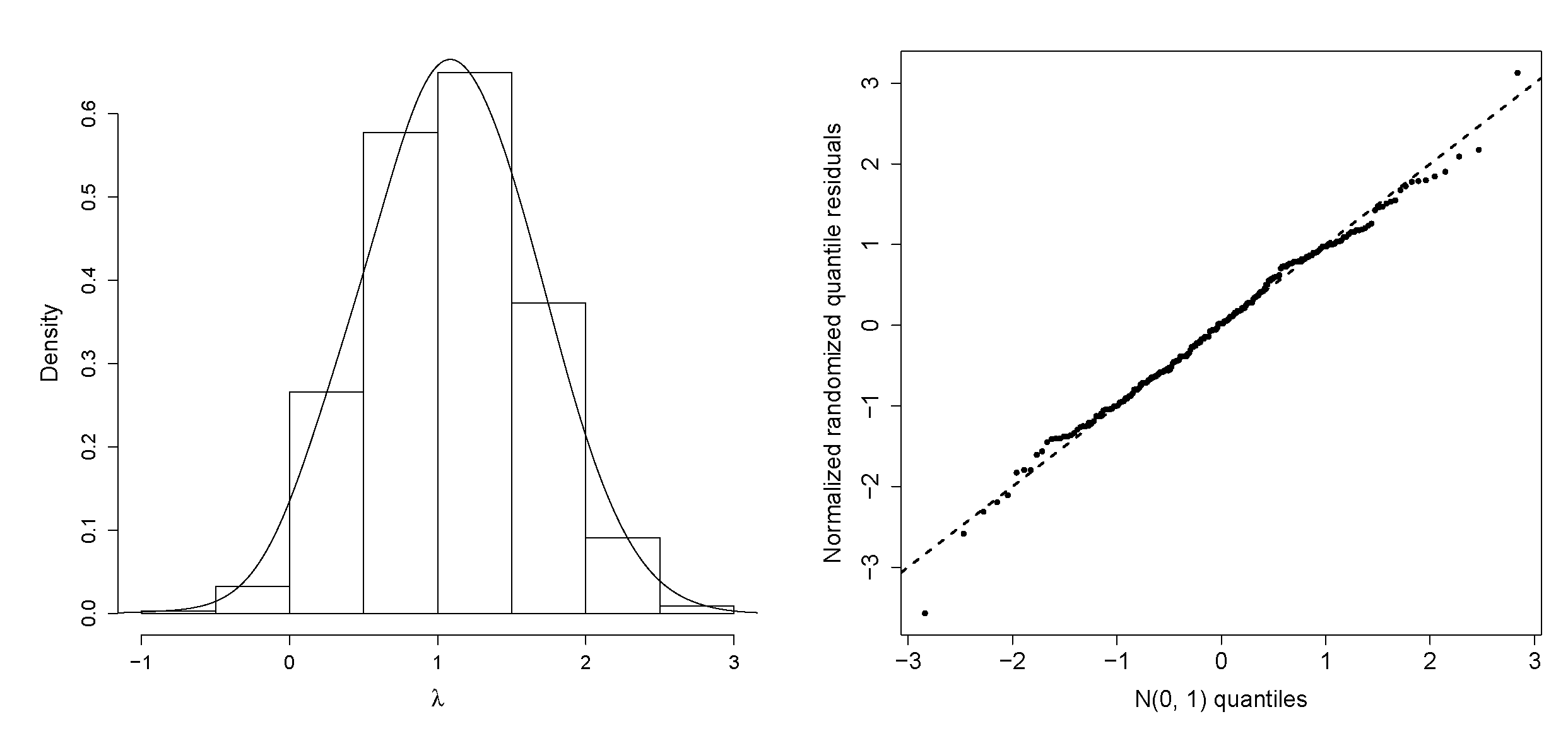
. All covariates are statistically significant at the significance level of 5% for all models. Figure 7 (left panel) displays the marginal posterior density of $\lambda$ in the Normal-GEV-CLL regression model, which is symmetric. Table 4 reveals that the posterior mean of $\lambda$ is 1.088, and a 95% HPD interval is $(0.0110,2.103)$. We fit the GJS-Student-t regression model [12] with four degrees of freedom and log–log link to the current data.

Table 5. Monte Carlo estimates of DIC, EAIC, EBIC, and LPML for Jhonson’s $S_B$ and GJS-Student-t regression models.

Model	Criteria
	DIC	EAIC	EBIC	LPML
GJS-t Student	−984.764	−976.786	−949.637	492.665
Jhonson’s	−986.343	−978.375	−951.226	491.750

reports the Monte Carlo estimates of DIC, EAIC, EBIC, and LPML for Jhonson’s $S_B$ and GJS-Student-t regression models. They indicate that the second regression is better than the first for these data, but it does not provide a better fit than the Normal-GEV-CLL regression model. The quantile–quantile (QQ) plot of the posterior normalized randomized quantile residuals for the last regression in Figure 7 (right panel) proves an acceptable fit [27,28].

We consider a Bayesian global influence methodology to identify the presence of outliers and/or influential observations under the general divergence measure [29]. Let $D_{\psi }(\pi ,{\pi }_{(-i)})$ be the $\psi$-divergence between $\pi$ and ${\pi }_{(-i)}$, where $\pi$ denotes the posterior distribution of $\mathbf{\vartheta }$ for the full dataset, and ${\pi }_{(-i)}$ the posterior distribution of $\mathbf{\vartheta }$ without the ith observation, namely:

$$D_{\psi }(\pi ,{\pi }_{(-i)})=\int \psi \left(\frac{\pi \left(\mathbf{\vartheta }\right|{\mathcal{D}}^{(-i)})}{\pi \left(\mathbf{\vartheta }\right|\mathcal{D})}\right)\pi \left(\mathbf{\vartheta }\right|\mathcal{D})d\mathbf{\vartheta }=E_{\mathbf{\vartheta }|\mathcal{D}}\left[\psi \left(\frac{CP{O}_i}{f(y_i;\mathbf{\vartheta })}\right)\right],$$

where $\psi$ is a convex function with $\psi \left(1\right)=0$. Different choices of $\psi$ are addressed by Dey and Birmiwal [30] and Pardo [31]. Here, $\psi \left(z\right)=-log\left(z\right)$ defines the Kullback–Leibler (K-L) divergence, $\psi \left(z\right)=(z-1)log\left(z\right)$ gives the J-distance, $\psi \left(z\right)=0.5|z-1|$ provides $L_1$ norm, and $\psi \left(z\right)=z{(1/z-1)}^2$ yields the ${\chi }^2$-square divergence. The divergence measure to verify whether a small subset of observations from the full data is influential or not follows the criterion by Peng and Dey [29] and Weiss [32]; see also Cancho et al. [15,33,34].

We calculate the Monte Carlo estimates of the divergence measures K-L, J, $L_1$, and ${\chi }^2$ for the posterior distribution of the parameters of the Normal-GEV-CLL regression models to detect possible influential points.

They are plotted in Figure 8 and identify the cases 39, 54, and 122 as possible influential observations in the posterior distribution.

Table 6. $\psi$-divergence measures for the Normal-GEV-CLL regression model.

Case	Mortality Rate	Sex	Race	State	K-L	J	${\mathit{L}}_1$	${\mathit{\chi }}^2$
39	0.11	Men	non-Hispanic white	Dist-Columbia	1.081	2.422	0.563	5.004
54	0.05	Women	Hispanic	Georgia	0.449	1.057	0.392	1.193
122	0.29	Women	non-Hispanic black	Nebraska	0.769	2.301	0.575	2.861

presents subjects having large K-L, J, $L_1$, and ${\chi }^2$.

For some cases, we refit the regression model to determine the impact of these observations on the posterior distribution of the parameters [15]. We eliminate each case individually and then two and three cases. The relative change (RC) of each estimate is $R{C}_{{\vartheta }_j}=({\widehat{\vartheta }}_j-{\widehat{\vartheta }}_{j\left(I\right)})/{\widehat{\vartheta }}_j\times 100\%$, where ${\widehat{\vartheta }}_{j\left(I\right)}$ is the posterior mean of ${\theta }_j$ (for $j=1,\dots ,9$) when the set I of observations is removed.

Table 7. RCs (in %) and the L and U limits of the $95\%$ HPD intervals after removing some cases.

Dropped		$\mathit{\lambda }$	${\mathit{\beta }}_0$	${\mathit{\beta }}_1$	${\mathit{\beta }}_{2_1}$	${\mathit{\beta }}_{2_2}$	${\mathit{\tau }}_0$	${\mathit{\tau }}_1$	${\mathit{\tau }}_{2_1}$	${\mathit{\tau }}_{2_2}$
none	Mean	1.088	−1.879	−0.398	0.343	0.797	2.641	0.671	0.545	−0.424
	L	0.011	−1.966	−0.444	0.265	0.716	1.906	0.376	0.225	−0.951
	U	2.103	−1.796	−0.363	0.430	0.894	3.352	0.968	0.846	0.101
{39}	RC	−39.0	−0.0	0.9	0.9	−0.3	−9.7	−21.4	25.2	−44.0
	L	−0.391	−1.960	−0.439	0.266	0.704	1.609	0.217	0.341	−0.744
	U	1.822	−1.797	−0.364	0.425	0.879	3.135	0.819	0.974	0.309
{54}	RC	−35.8	0.1	0.8	1.5	−0.1	−8.6	−20.7	22.4	−41.5
	L	−0.343	−1.964	−0.437	0.261	0.715	1.751	0.232	0.382	−0.777
	U	1.763	−1.802	−0.363	0.423	0.882	3.196	0.828	0.998	0.225
{122}	RC	23.3	−0.2	1.2	0.0	−1.4	5.2	17.2	−7.5	7.3
	L	0.305	−1.961	−0.442	0.260	0.692	2.040	0.475	0.195	−0.950
	U	2.324	−1.798	−0.363	0.420	0.867	3.435	1.059	0.801	0.050
{39,54}	RC	−50.7	−0.7	0.5	−3.2	−2.4	−10.3	−20.6	13.9	−37.8
	L	−0.528	−1.938	−0.436	0.251	0.693	1.693	0.262	0.333	−0.777
	U	1.602	−1.790	−0.363	0.402	0.859	3.179	0.835	0.929	0.243
{39,122}	RC	−17.0	−0.4	2.1	0.1	−1.8	−4.7	−5.2	17.1	−35.6
	L	−0.277	−1.955	−0.444	0.268	0.700	1.779	0.328	0.321	−0.807
	U	1.927	−1.794	−0.370	0.426	0.869	3.253	0.924	0.937	0.202
{54,122}	RC	12.1	−1.1	0.8	−5.6	−4.0	4.4	16.9	−17.5	11.8
	L	0.246	−1.933	−0.439	0.248	0.686	2.077	0.492	0.149	−0.978
	U	2.201	−1.789	−0.359	0.388	0.842	3.449	1.052	0.734	−0.034
{39,54,122}	RC	−29.7	−1.0	1.8	−3.7	−3.6	−5.5	−5.6	4.7	−31.0
	L	−0.388	−1.930	−0.444	0.261	0.694	1.782	0.338	0.270	−0.830
	U	1.848	−1.787	−0.370	0.402	0.846	3.323	0.947	0.883	0.223

reports the RCs after removing some observations, and the lower (L) and upper (U) limits of the $95\%$ HPD intervals of the new estimates. In general, the significance of the parameter estimates does not change after removing set I at the level of 5%.

We estimate the median of the mortality rate for eight patients A, B, C, D, E, and F with specified characteristics in

Table 8. Mortality rate estimates and the $95\%$ HPD intervals for six colorectal cancer patients.

Patient	$\mathbf{Sex}$	$\mathbf{Race}$	Mortality Rate
			Mean	Median	HPD (95%) Interval
A	Men	Hispanic	0.142	0.142	(0.131, 0.153)
B	Women	Hispanic	0.098	0.098	(0.090, 0.105)
C	Men	non-Hispanic white	0.194	0.194	(0.188, 0.200)
D	Women	non-Hispanic white	0.135	0.135	(0.131, 0.138)
E	Men	non-Hispanic black	0.287	0.287	(0.275, 0.299)
F	Women	non-Hispanic black	0.204	0.204	(0.195, 0.212)

. These numbers refer to the Bayes estimates under the quadratic and absolute loss functions and the $95\%$ HPD intervals for the median mortality. For example, the median mortality rates are 0.147 and 0.276 for patient A of gender male and race Hispanic and patient E of gender male and race Hispanic, respectively. This difference can be seen in Figure 9, and in the posterior distribution of the median mortality rate of the other patients.

6. Conclusions

We provided some mathematical properties of the new normal-generalized extreme value (Normal-GEV) distribution, and proposed a new and flexible regression model for proportional variables. This regression model is an alternative to the well-known beta regression model [2]. Some simulation studies and Bayesian procedures were developed to analyze a real dataset and they showed that the proposed regression is very competitive and useful for inferential and diagnostic problems involving bounded response variables and covariate variables.