Article

The Bivariate Unit-Sinh-Normal Distribution and Its Related Regression Model

by
Guillermo Martínez-Flórez
1,*,†,
Artur J. Lemonte
2,*,†,
Germán Moreno-Arenas
3 and
Roger Tovar-Falón
1,*
1
Departamento de Matemáticas y Estadística, Facultad de Ciencias Básicas, Universidad de Córdoba, Monteria 230002, Colombia
2
Departamento de Estatística, Universidade Federal do Rio Grande do Norte, Natal 59078970, RN, Brazil
3
Escuela de Matemáticas, Universidad Industrial de Santander, Bucaramanga 680006, Colombia
*
Authors to whom correspondence should be addressed.
These authors contributed equally to this work.
Mathematics 2022, 10(17), 3125; https://doi.org/10.3390/math10173125
Submission received: 2 July 2022 / Revised: 10 August 2022 / Accepted: 18 August 2022 / Published: 31 August 2022

Abstract

:
In this paper, a new bivariate absolutely continuous probability distribution is introduced. The new distribution, which is called the bivariate unit-sinh-normal (BVUSHN) distribution, arises by applying a transformation to the bivariate Birnbaum–Saunders distribution (BVBS). The main properties of the new proposal are studied in detail. In addition, from the new distribution, the BVUSHN regression model is also introduced. For both the bivariate probability distribution and the respective associated regression model, parameter estimation is conducted from a classical approach by using the maximum likelihood method together with the two-step estimation method. A small Monte Carlo simulation study is carried out to evaluate the behavior of the used estimation method and the properties of the estimators. Finally, for illustrative purposes, two applications with real data are presented in which the usefulness of the proposals is evidenced.

1. Introduction

Birnbaum and Saunders [1,2] developed an important two-parameter lifetime distribution for fatigue failure caused under dynamic load. The probability density function (pdf) of the Birnbaum–Saunders (BS) distribution is given by
f T ( t ) = ϕ ( a t ) A t , t > 0 ,
where a t = α 1 ( t / β β / t ) , A t = t 3 / 2 ( t + β ) / [ 2 α β ] , ϕ ( · ) is the pdf of the standard normal distribution, α > 0 is the shape parameter, and  β > 0 is a scale parameter. We use the conventional notation to denote this distribution, that is, T BS ( α , β ) . Extensions of the BS distribution have been studied for many authors, for example, [3,4,5,6,7,8,9].
In addition to the work mentioned above, recent proposals were made by Balakrishnan and Kundu [10], who made a detailed review of the developments that have taken place in relation to the BS distribution. In particular, the authors addressed different aspects, including interpretations, constructions, generalizations, inference processes, and extensions to multivariate cases, among others. The authors also presented some open problems that could be considered in future research. Furthermore, Athayde et al. [11] studied the failure rate shape of the Birnbaum–Saunders-logistic distribution. In addition, the authors discussed and compared some robustness issues related to the Birnbaum–Saunders, Birnbaum–Saunders-logistic, and Birnbaum–Saunders-t distributions. On the other hand, Arrué et al. [12] built an extension of the BS distribution from the skew-normal model and gained flexibility in skewness and kurtosis. The characterization of this new distribution was presented and they illustrated the usefulness of their proposal with a motivating example of fatigue life data.
A more recent extension of the BS distribution to the case of bimodal data was presented by Reyes et al. [13]. This proposal has proven to be useful for the analysis of data from the environment and medical sciences, which demonstrates the wide field of applicability for this model in the different areas of knowledge by considering not only data from engineering, for example.
The BS distribution has also been extended to models suitable for fitting data in the interval ( 0 , 1 ) as rates, proportions, or indices. Mazucheli et al. [14], for example, presented a type of BS distribution with support in the unit interval ( 0 , 1 ) , which is a new alternative to the beta and Kumaraswamy distributions. These authors have called it as unit-Birnbaum–Saunders (UBS) distribution. The UBS distribution is obtained from the transformation X = exp ( T ) , where T BS ( α , β ) . The pdf of the UBS distribution is given by
f ( x ) = 1 2 x α β 2 π β log x 1 / 2 + β log x 3 / 2 exp 1 2 α 2 log x β + β log x + 2 ,
where x ( 0 , 1 ) , α > 0 is the shape parameter, and  β > 0 is a scale parameter. The corresponding cumulative distribution function (cdf) is given by
F ( x ) = 1 Φ 1 α log x β 1 / 2 β log x 1 / 2 , x ( 0 , 1 ) ,
where Φ ( · ) is the cdf of the standard normal distribution. We use the notation X UBS ( α , β ) .
The BS distribution has also been used to define linear regression models, known as log-BS models. In this framework, it is assumed that Y = log ( T ) , where T BS ( α , β ) , and the errors of the log-linear model follow the sinh-normal (SHN) distribution of Rieck and Nedelman [15]. The pdf of the SHN distribution is given by
φ ( y ) = B y ϕ ( b y ) , y R ,
where b y = b ( y ; α , μ , σ ) = ( 2 / α ) sinh ( ( y μ ) / σ ) , B y = B ( y ; α , μ , σ ) = σ 1 ( 2 / α ) cosh ( ( y μ ) / σ ) , α > 0 is the shape parameter, μ is a location parameter, and  σ > 0 is a scale parameter. We use the notation Y SHN ( α , μ , σ ) . Extensions of the SHN distribution are reported in Martínez-Flórez et al. [8], Barros et al. [16], Leiva et al. [17], Lemonte [18], and and Santana et al. [19].
Extensions of the BS distribution to the bivariate setup were given by Kundu et al. [20] and, for the multivariate case, Lemonte et al. [21] introduced the multivariate skew-normal distribution. Likewise, for the log-BS regression model, Lemonte [22] proposed the multivariate BS regression model, Kundu [23] studied the bivariate SHN distribution, and Martínez-Flórez et al. [24] considered the asymmetric multivariate BS regression model. In addition, Martínez-Flórez et al. [25] proposed an exponentiated multivariate extension of the BS log-linear model, that is, an extension to the alpha-power family of distribution.
To study the relationship between variables when the dependent variable is observed in the unit interval, such as indices, rates, or proportions, the most widely known and used model is the beta regression model. Other authors developed works in this same direction using the beta distribution; see, for example, [26,27,28,29,30,31,32]. On the other hand, situations in which the limits of the interval ( 0 , 1 ) are included in the support of the response variable have also been considered; see, for example, [33,34,35,36,37].
The chief goal of this paper is to introduce a bivariate regression model to deal with response variables in the unit interval. To do so, we first introduce a bivariate probability distribution supported on the unit interval which arises from the bivariate SHN distribution. The article is organized as follows. Section 2 presents the bivariate BS and SHN distributions. The bivariate UBS distribution is introduced in Section 3, and some of its structural properties are also derived. The results of a simulation study and its respective discussion are presented in Section 6. In Section 4, we introduce the bivariate unit SHN distribution, and we derive some of its properties. The bivariate unit SHN regression model is introduced in Section 5. Applications to real data are provided in Section 7.

2. The Bivariate BS and SHN Distributions

Kundu et al. [20] extended the univariate BS distribution to the bivariate case. The bivariate random vector ( T 1 , T 2 ) follows a bivariate BS distribution if it can be expressed as
( T 1 , T 2 ) = β 1 α 1 2 Z 1 + α 1 2 Z 1 2 + 1 2 , β 2 α 2 2 Z 2 + α 2 2 Z 2 2 + 1 2 ,
where the bivariate random vector ( Z 1 , Z 2 ) follows a bivariate normal distribution with parameters ( 0 , 0 , 1 , 1 , ρ ) and  1 < ρ < 1 . It follows that the cdf of the bivariate BS distribution is given by
F T 1 , T 2 ( t 1 , t 2 ) = Φ 2 ( a t 1 , a t 2 ; ρ ) , t 1 > 0 , t 2 > 0 ,
where Φ 2 ( · ) is the cdf of the bivariate normal distribution and 
a t j = a t j ( α j , β j ) = 1 α j t j β j β j t j , j = 1 , 2 .
Hence, the joint pdf of ( T 1 , T 2 ) can be written as
f T 1 , T 2 ( t 1 , t 2 ) = ϕ 2 ( a t 1 , a t 2 ; ρ ) A t 1 A t 2 ,
where ϕ 2 ( x , y ; ρ ) denotes the pdf of the bivariate standard normal distribution and
A t j = t j 3 / 2 [ t j + β j ] 2 α j β j 1 / 2 , j = 1 , 2 .
We use the notation ( T 1 , T 2 ) BVBS ( α 1 , α 2 , β 1 , β 2 , ρ ) . Similarly, the bivariate SHN distribution of the random vector ( Y 1 , Y 2 ) , studied by Kundu [23], is defined by the joint distribution function
G Y 1 , Y 2 ( y 1 , y 2 ) = Φ 2 ( b y 1 , b y 2 ; ρ ) , y 1 R , y 2 R ,
where b y j = b ( y j ; α j , μ j , σ j ) for j = 1 , 2 . Hence, the joint pdf of ( Y 1 , Y 2 ) can be written as
g Y 1 , Y 2 ( y 1 , y 2 ) = ϕ 2 ( b y 1 , b y 2 ; ρ ) B y 1 B y 2 , y 1 R , y 2 R ,
where B y j = B ( y j ; α j , μ j , σ j ) . The notation ( Y 1 , Y 2 ) BVSHN ( α 1 , α 2 , μ 1 , μ 2 , σ 1 , σ 2 , ρ ) is used to denote this distribution. The reader is referred to Kundu et al. [20] and Kundu [23] for more details about the BVBS and BVSHN distributions, respectively.

3. The Bivariate UBS Distribution

We now introduce the bivariate UBS distribution and study some of its properties and the process of estimating its parameters. The bivariate random vector ( X 1 , X 2 ) is said to have a bivariate UBS distribution with parameters α 1 , β 1 , α 2 , β 2 , and ρ if the joint cdf of ( X 1 , X 2 ) is given by
F X 1 , X 2 ( x 1 , x 2 ) = 1 Φ ( λ x 1 ) Φ ( λ x 2 ) + Φ 2 ( λ x 1 , λ x 2 ; ρ ) ,
where x 1 ( 0 , 1 ) , x 2 ( 0 , 1 ) , and 
λ x j = λ x j ( α j , β j ) = 1 α j log x j β j β j log x j .
Hence, the joint pdf of ( X 1 , X 2 ) which is obtained by deriving (1) can be expressed as
f X 1 , X 2 ( x 1 , x 2 ) = ϕ 2 ( λ x 1 , λ x 2 ; ρ ) Λ x 1 Λ x 2 ,
where
Λ x j = ( log x j ) 3 / 2 [ β j log x j ] 2 x j α j β j 1 / 2 , j = 1 , 2 .
For the joint pdf given in (2), we use the notation BVUBS ( α 1 , α 2 , β 1 , β 2 , ρ ) , where ρ is the correlation coefficient. The bivariate distribution ( X 1 , X 2 ) BVUBS ( α 1 , α 2 , β 1 , β 2 , ρ ) is obtained from the vector transformation ( X 1 , X 2 ) = ( exp ( T 1 ) , exp ( T 2 ) ) , where ( T 1 , T 2 ) BVBS ( α 1 , α 2 , β 1 , β 2 , ρ ) .
From the previous definition, it follows that ( Z 1 , Z 2 ) BN ( 0 , 0 , 1 , 1 , ρ ) with
( Z 1 , Z 2 ) = 1 α 1 log X 1 β 1 β 1 log X 1 , 1 α 2 log X 2 β 2 β 2 log X 2 ,
where BN ( 0 , 0 , 1 , 1 , ρ ) denotes the bivariate standard normal distribution with correlation coefficient ρ . Therefore, for the marginal distributions, it follows that
Z j = 1 α j log X j β j β j log X j N ( 0 , 1 ) and Z j 2 χ 1 2 , for j = 1 , 2 ,
and, hence, if  ( X 1 , X 2 ) BVUBS ( α 1 , α 2 , β 1 , β 2 , ρ ) , then
( T 1 , T 2 ) = ( log X 1 , log X 2 ) BVBS ( α 1 , α 2 , β 1 , β 2 , ρ ) .
We have the following theorem.
Theorem 1.
Let ( X 1 , X 2 ) BVUBS ( α 1 , α 2 , β 1 , β 2 , ρ ) . Hence:
(i) 
X j UBS ( α j , β j ) , for j = 1 , 2 .
(ii) 
The cdf of X 1 , given X 2 = x 2 , is
F X 1 X 2 = x 2 ( x 1 X 2 = x 2 ) = 1 Φ λ x 1 ρ λ x 2 1 ρ 2 .
(iii) 
The pdf of X 1 , given X 2 = x 2 , is
f X 1 X 2 = x 2 ( x 1 X 2 = x 2 ) = 1 2 π 1 ρ 2 exp 1 2 λ x 1 ρ λ x 2 1 ρ 2 2 .
(iv) 
The joint survival function of ( X 1 , X 2 ) is
S X 1 , X 2 ( x 1 , x 2 ) = Φ ( λ x 1 ) + Φ ( λ x 2 ) Φ 2 ( λ x 1 , λ x 2 ; ρ ) .
Remark 1.
We can generate random samples from the BVUBS ( α 1 , α 2 , β 1 , β 2 , ρ ) distribution according to the algorithm described below:
(i) 
For j = 1 , 2 , obtain T j following the described algorithm in Kundu et al. [20].
(ii) 
For each value of T j , compute
X j = exp ( T j ) , j = 1 , 2 .
Hence, ( X 1 , X 2 ) BVUBS ( α 1 , α 2 , β 1 , β 2 , ρ ) .
Since the marginal X j UBS ( α j , β j ) for j = 1 , 2 , the mean and variance of X j are
E ( X j ) = 2 α j 2 β j + 2 α j 2 β j + 1 + 1 2 ( 2 α j 2 β j + 1 ) exp 2 α j 2 β j + 1 1 α j 2 ,
V a r ( X j ) = 4 α j 2 β j + 4 α j 2 β j + 1 + 1 2 ( 4 α j 2 β j + 1 ) exp 4 α j 2 β j + 1 1 α j 2 E 2 ( X j ) .
The product moments of ( X 1 , X 2 ) , say, m r s = E ( X 1 r X 2 s ) , are complicated to obtain in closed-form expression and, hence, they have to be obtained from numerical calculations. However, for  ρ = 0 , it follows that
E ( X 1 X 2 ) = exp j = 1 2 2 α j 2 β j + 1 1 α j 2 j = 1 2 2 α j 2 β j + 2 α j 2 β j + 1 + 1 2 ( 2 α j 2 β j + 1 ) .
We say that a function defined in R 2 is totally positive of order 2 (abbreviated T P 2 ) for  x 1 < x 2 and y 1 < y 2 , with x , y R if
g ( x 1 , y 1 ) g ( x 2 , y 2 ) g ( x 2 , y 1 ) g ( x 1 , y 2 ) .
We have the following theorem.
Theorem 2.
Let ( X 1 , X 2 ) BVUBS ( α 1 , α 2 , β 1 , β 2 , ρ ) . For  0 < ρ < 1 , we have that ( X 1 , X 2 ) is T P 2 .
Proof. 
The proof follows from the fact that for ( X 1 , X 2 ) BVUBS ( α 1 , α 2 , β 1 , β 2 , ρ ) it follows that ( T 1 , T 2 ) = ( log X 1 , log X 2 ) BVBS ( α 1 , α 2 , β 1 , β 2 , ρ ) . Furthermore, let f BVBS ( · ) and f BVUBS ( · ) be the joint pdfs of the BVBS and BVUBS distributions, respectively. Then, f BVUBS ( log x 1 , log x 2 ) = 1 x 1 x 2 f BVBS ( log x 1 , log x 2 ) . Since ( T 1 , T 2 ) is TP2, then for 0 < ρ < 1 and for x 11 < x 12 and x 21 < x 22 , we have that 0 < log x 12 < log x 11 and 0 < log x 22 < log x 21 . Note that
f BVBS ( log x 12 , log x 22 ) f BVBS ( log x 11 , log x 21 ) f BVBS ( log x 11 , log x 22 ) f BVBS ( log x 12 , log x 21 ) 0 ,
and, hence,
f BVUBS ( x 11 , x 21 ) f BVUBS ( x 12 , x 22 ) f BVUBS ( x 12 , x 21 ) f BVUBS ( x 11 , x 22 ) 0 .
Therefore, for  0 < ρ < 1 , ( X 1 , X 2 ) is TP2.    □

Parameter Estimation

Estimating the unknown parameters of a parametric model lies at the heart of distribution theory and its applications. In this section, the estimation of the BVUBS model parameters is investigated by the maximum likelihood (ML) method.
Let { ( x 11 , x 12 ) , , ( x n 1 , x n 2 ) } be a sample of size n from the BVUBS ( α 1 , α 2 , β 1 , β 2 , ρ ) distribution. The log-likelihood function for the parameter vector θ = ( α 1 , α 2 , β 1 , β 2 , ρ ) is given by
( θ ) = n log ( α 1 α 2 β 1 β 2 ) n 2 log ( 1 ρ 2 ) + i = 1 n j = 1 2 log β j log x i j 1 / 2 + β j log x i j 3 / 2 1 2 ( 1 ρ 2 ) i = 1 n [ j = 1 2 1 α j 2 log x i j β j β j log x i j 2 2 ρ j = 1 2 1 α j log x i j β j β j log x i j ] .
We have that
log X j β j β j log X j N ( 0 , α j 2 ) , for j = 1 , 2 .
Since ( Z 1 , Z 2 ) BN ( 0 , 0 , 1 , 1 , ρ ) , it follows that
log X 1 β 1 β 1 log X 1 , log X 2 β 2 β 2 log X 2 N 2 0 0 , Σ ,
where
Σ = α 1 2 α 1 α 2 ρ α 1 α 2 ρ α 2 2 .
We have that, given β 1 and β 2 , the ML estimators of α 1 , α 2 , and ρ become
α ^ j ( β j ) = s j β j + β j r j 2 1 / 2 , j = 1 , 2 ,
where s j = ( 1 / n ) i = 1 n ( log x j ) , r j = [ ( 1 / n ) i = 1 n ( log x j ) 1 ] 1 , and
ρ ^ ( β 1 , β 2 ) = i = 1 n j = 1 2 log x i j β j β j log x i j j = 1 2 i = 1 n log x i j β j β j log x i j 2 .
To estimate β 1 and β 2 , we consider the following profiled log-likelihood function
p ( β 1 , β 2 ) = n log ( β 1 β 2 α ^ 1 ( β 1 ) α ^ 2 ( β 2 ) ) n 2 log ( 1 ρ ^ ( β 1 , β 2 ) ) + i = 1 n j = 1 2 log β j log x i j 1 / 2 + β j log x i j 3 / 2 .
The ML estimates for β 1 and β 2 need to be obtained through a numerical maximization using optimization algorithms such as, for example, the Newton–Raphson iterative technique. The optimization algorithms require the specification of initial values to be used in the iterative scheme. Our suggestion is to use as initial guesses the estimates obtained from the modified moments of the marginal distributions of X j for j = 1 , 2 , given that X j UBS ( α j , β j ) . More details about these values, which are denoted by α ¯ j , β ¯ j , and ρ ¯ , can be found in Kundu et al. [20].
Let θ ^ = ( α ^ 1 , α ^ 2 , β ^ 1 , β ^ 2 , ρ ^ ) denote the ML estimator of θ = ( α 1 , α 2 , β 1 , β 2 , ρ ) . For n , we have that n ( θ ^ θ ) N 5 ( 0 5 , I 1 ( θ ) ) , where I ( θ ) is the Fisher information matrix, whose elements are the same as those given for the Fisher information matrix of the BVBS distribution provided in Kundu et al. [20], just replacing T j by log X j .

4. The Bivariate Unit SHN Distribution

The SHN distribution studied by Rieck and Nedelman [15] is defined on the set of real numbers. Similarly, the bivariate SHN distributions of Kundu [23] and Martínez-Flórez et al. [24] are defined on R 2 . Therefore, its application to sets of variables that are distributed between zero and one would not always be a convenient option.
We now introduce a bivariate distribution for rates or proportions as an alternative to bivariate datasets supported by the unit rectangle ( 0 , 1 ) × ( 0 , 1 ) . Since the SHN distribution is defined on the set of real numbers, to obtain an adequate transformation that allows us to define a random variable with a distribution in the unit interval ( 0 , 1 ) , we use the log-log complement transformation. We say that the variable Y follows the unit SHN (USHN) distribution with parameters ( α , μ , σ ) if 
Z = 2 α sinh log ( log ( 1 Y ) ) μ σ N ( 0 , 1 ) .
Thus, the pdf of a random variable Y with a USHN distribution is given by
φ ( y ) = Ω y ϕ ω y , y ( 0 , 1 )
with
Ω y = Ω ( y ; α , μ , σ ) = 2 α cosh log ( log ( 1 y ) ) μ σ σ ( 1 y ) log ( 1 y ) 1 , ω y = ω ( y ; α , μ , σ ) = 2 α sinh log ( log ( 1 y ) ) μ σ ,
where α > 0 is the shape parameter, μ is a location parameter, and  σ > 0 is a scale parameter. We use the notation Y USHN ( α , μ , σ ) .
The cdf of the random variable Y USHN ( α , μ , σ ) takes the form
F ( y ) = F SHN ( log ( log ( 1 y ) ) ) = Φ 2 α sinh log ( log ( 1 y ) ) μ σ ,
where F SHN ( · ) is the cdf of the SHN ( α , μ , σ ) distribution. In addition, if  Z N ( 0 , 1 ) , then
Y = 1 e e μ + σ sinh 1 α Z 2 USHN ( α , μ , σ ) .
Finally, the generation of a random variable with a USHN ( α , γ , σ ) distribution can be obtained from the previous expression.

Bivariate Extension

The bivariate USHN distribution can be directly obtained from the transformation
Y j = 1 e e μ j + σ j sinh 1 α j Z j 2 with Z j N ( 0 , 1 ) , j = 1 , 2 .
The bivariate vector ( Y 1 , Y 2 ) is said to have a bivariate USHN distribution with parameters α 1 , μ 1 , σ 1 , α 2 , μ 2 , σ 2 , and ρ if the joint cdf of ( Y 1 , Y 2 ) is given by
F Y 1 , Y 2 ( y 1 , y 2 ) = Φ 2 ( ω y 1 , ω y 2 ; ρ ) ,
where
ω y j = ω ( y j ; α j , μ j , σ j ) = 2 α j sinh log ( log ( 1 y j ) ) μ j σ j .
The joint pdf of ( Y 1 , Y 2 ) which follows from (3) can be expressed as
f Y 1 , Y 2 ( y 1 , y 2 ) = ϕ 2 ( ω y 1 , ω y 2 ; ρ ) Ω y 1 Ω y 2 ,
where
Ω y j = Ω ( y j ; α j , μ j , σ j ) = 2 α j cosh log ( log ( 1 y j ) ) μ j σ j σ j ( 1 y j ) log ( 1 y j ) 1 , j = 1 , 2 .
The notation used is ( Y 1 , Y 2 ) BVUSHN ( α 1 , μ 1 , σ 1 , α 2 , μ 2 , σ 2 , ρ ) , where ρ is the correlation coefficient. From the previous definition, it follows that
( Z 1 , Z 2 ) BN ( 0 , 0 , 1 , 1 , ρ ) ,
where
Z j = 2 α j sinh log ( log ( 1 Y j ) ) μ j σ j , j = 1 , 2 .
We have the following theorems.
Theorem 3.
Let ( Y 1 , Y 2 ) BVUSHN ( α 1 , μ 1 , σ 1 , α 2 , μ 2 , σ 2 , ρ ) . Hence:
(i) 
Y j U S H N ( α j , μ j , σ j ) , for j = 1 , 2 .
(ii) 
The cdf of Y 1 , given Y 2 = y 2 , is
F Y 1 Y 2 = y 2 ( y 1 Y 2 = y 2 ) = Φ ω y 1 ρ ω y 2 1 ρ 2 .
(iii) 
The pdf of Y 1 , given Y 2 = y 2 , is
f Y 1 Y 2 = y 2 ( y 1 Y 2 = y 2 ) = Ω y 1 2 π 1 ρ 2 exp 1 2 ω y 1 ρ ω y 2 1 ρ 2 2 .
(iv) 
The joint survival function of ( Y 1 , Y 2 ) is
S Y 1 , Y 2 ( y 1 , y 2 ) = 1 Φ ( ω y 1 ) Φ ( ω y 2 ) + Φ 2 ( ω y 1 , ω y 2 ; ρ ) .
Theorem 4.
If ( Y 1 , Y 2 ) BVUSHN ( α 1 , μ 1 , σ 1 , α 2 , μ 2 , σ 2 , ρ ) , then the conditional hazard function of Y 1 , given Y 2 = y 2 , is a non-decreasing function of y 1 , for all values of y 2 and ρ when μ 1 > 0 and σ 1 < 1 .
Marshall [38] defined the bivariate hazard rate of Y 1 and Y 2 as
h ( y 1 , y 2 ) = y 1 , y 2 log P ( Y 1 > y 1 , Y 2 > y 2 ) = ( h 1 ( y 1 , y 2 ) , h 2 ( y 1 , y 2 ) ) .
Theorem 5.
If ( Y 1 , Y 2 ) BVUSHN ( α 1 , μ 1 , σ 1 , α 2 , μ 2 , σ 2 , ρ ) , then:
(i) 
For y 2 fixed and σ 1 < 1 , h 1 ( y 1 , y 2 ) is a non-decreasing function of y 1 .
(ii) 
For y 1 fixed and σ 2 < 1 , h 2 ( y 1 , y 2 ) is a non-decreasing function of y 2 .
Remark 2.
We can generate samples from the BVUSHN ( α 1 , μ 1 , σ 1 , α 2 , μ 2 , σ 2 , ρ ) distribution according to the algorithm described below:
(i) 
For j = 1 , 2 , generate Z j according to the algorithm given by Kundu [23];
(ii) 
For each value of Z j , compute
Y j = 1 e e μ j + σ j sinh 1 α j Z j 2 , j = 1 , 2 .
Hence, ( Y 1 , Y 2 ) BVUSHN ( α 1 , μ 1 , σ 1 , α 2 , μ 2 , σ 2 , ρ ) .

5. Bivariate Unit SHN Regression Model

Suppose that Y 1 = ( Y 11 , Y 12 ) , , Y n = ( Y n 1 , Y n 2 ) are n independent bivariate vectors of proportions, where for each bivariate vector we assume that
Y i = ( Y i 1 , Y i 2 ) BVUSHN ( α 1 , X i β 1 , σ 1 , α 2 , X i β 2 , σ 2 , ρ ) , i = 1 , , n ,
where X i = ( x i 1 , x i 2 , , x i p ) is a p-dimensional vector with values of the explanatory variables associated with the j-th observable response y j , such that Y i j USHN ( α j , X i β j , σ j ) . In addition, β j is a vector of size p of unknown parameters for j = 1 , 2 . In other words, we assume that, for each i = 1 , 2 , , n and j = 1 , 2 , the location parameter of the response variable Y i j satisfies the functional relationship
log ( log ( 1 μ i j ) ) = X i j β j ,
which corresponds to the log-log complement link function.
Let Y = vec ( Y 1 , Y 2 ) be of size 2 n , X = ( X 1 , X 2 , , X n ) and X * = diag ( X , X ) be of size 2 n × 2 p , where vec ( · ) is the vec operator, and β = ( β 1 , β 2 ) = ( β 1 , β 2 , , β 2 p ) be a 2 p -vector of unknown parameters.

5.1. Parameter Estimation

The estimation of the parameter vector θ = ( α 1 , α 2 , σ 1 , σ 2 , β , ρ ) of size 5 + 2 p can be carried out by maximizing the log-likelihood function
( θ ) = i = 1 n i ( θ ) ,
where
i ( θ ) = log ( ϕ 2 ( ω ( y i 1 ; α 1 , X i 1 β , σ 1 ) , ω ( y i 2 ; α 2 , X i 2 β , σ 2 ) ; ρ ) ) + j = 1 2 log Ω ( y i j ; α j , X i j β , σ j ) ,
with
ω ( Y i j ; α j , X i j β , σ j ) = 2 α j sinh log ( log ( 1 Y i j ) ) X i j β σ j N ( 0 , 1 ) .
We have that
V i j = log ( log ( 1 Y i j ) ) X i j β σ j SHN ( α j , 0 , 1 ) ,
for i = 1 , 2 , , n and j = 1 , 2 . Thus,
e V i 1 e V i 1 , e V i 2 e V i 2 N 2 0 0 , α 1 2 α 1 α 2 ρ α 1 α 2 ρ α 2 2 .
For σ 1 , σ 2 , and β fixed, with 
g ( y i j ; X i j β , σ j ) = e v i j e v i j ,
it follows that
α ^ j ( β , σ j ) = 1 n i = 1 n g 2 ( y i j ; X i j β , σ j ) 1 / 2 ,
and
ρ ^ ( β , σ 1 , σ 2 ) = i = 1 n g ( y i 1 ; X i 1 β , σ 1 ) g ( y i 2 ; X i 2 β , σ 2 ) i = 1 n g 2 ( y i 1 ; X i 1 β , σ 1 ) i = 1 n g 2 ( y i 2 ; X i 2 β , σ 2 ) .
Thus, to estimate σ 1 , σ 2 , and β , we use the profiled likelihood approach; that is, the estimates of these parameters are obtained by maximizing
p ( β , σ 1 , σ 2 ) = ( α ^ 1 ( β , σ 1 ) , σ 1 , β , α ^ 2 ( β , σ 2 ) , σ 2 , ρ ^ ( β , σ 1 , σ 2 ) ) ,
regarding σ 1 , σ 2 , and β . This maximization procedure requires iterative numerical methods such as Newton–Raphson or quasi-Newton.
Denoting the estimators of β , σ 1 , and σ 2 by β ^ , σ ^ 1 , and σ ^ 2 , respectively, then the estimators of α 1 , α 2 ,and ρ are given by α ^ 1 = α ^ 1 ( β ^ , σ ^ 1 ) , α ^ 2 = α ^ 2 ( β ^ , σ ^ 2 ) , and ρ ^ = ρ ^ ( β ^ , σ ^ 1 , σ ^ 2 ) , respectively. The elements of the Fisher information matrix can be obtained by calculating the second derivatives of the log-likelihood function regarding the parameters of the model and thus finding the expectation numerically.

5.2. Two-Step Estimation

From (5), it follows that
log ( log ( 1 Y i j ) ) = X i j β + σ j V i j SHN ( α j , X i j β , σ j ) ,
for i = 1 , 2 , , n and j = 1 , 2 ; that is, the bivariate USHN regression model can be seen as
W i j = log ( log ( 1 Y i j ) ) = X i j β + ϵ i j = μ i j + ϵ i j ,
where ϵ i j SHN ( α j , 0 , σ j ) for i = 1 , 2 , , n and j = 1 , 2 . Since W i j SHN ( α j , μ i j , σ j ) for i = 1 , 2 , , n and j = 1 , 2 , we can use the two-step method presented in Kundu [23] to estimate the parameters of the bivariate USHN regression model.
The two-step estimation method was provided by Joe [39] and it is an interesting procedure because it reduces the dimension of the parameter space in each of its stages. In our case, the estimation of the parameters will be determined in two independent stages, where in the first stage, the estimates of the marginals of each variable under study will be obtained, that is, 2 + p will be estimated in the marginal distribution and, in the second stage, the association parameter ρ will be estimated. The ML estimators obtained by the two-stage procedure are consistent and the variance-covariance matrix is obtained using the methodology presented in Joe [39].
Expressing the joint cdf of W 1 and W 2 in terms of the normal copula, we have that
F W 1 W 2 ( w 1 , w 2 ) = Φ 2 ( a ( w 1 ; α 1 , μ W 1 , σ 1 ) , a ( w 2 ; α 2 , μ W 2 , σ 2 ) ; ρ ) = C G ( F W 1 ( w 1 ) , F W 2 ( w 2 ) ; ρ ) = C G ( u , v ; ρ ) ,
where C G ( · , · ; ρ ) denotes the Gaussian copula. In addition, u , v U ( 0 , 1 ) and F W j ( · ) for j = 1 , 2 is the cdf of W j . Then, let c G ( u , v ; ρ ) = 2 C G ( u , v ; ρ ) / u v be the pdf of the Gaussian copula. It follows that the log-likelihood function can be expressed as
( θ ) = i = 1 n log c G F ( w i 1 ; α 1 , μ i 1 , σ 1 ) , F ( w i 2 ; α 2 , μ i 2 , σ 2 ) ; ρ + i = 1 n log f ( w i 1 ; α 1 , μ i 1 , σ 1 ) + i = 1 n log f ( w i 2 ; α 2 , μ i 2 , σ 2 ) ,
where f ( w i j ; α j , μ i j , σ j ) is the pdf of W i j for i = 1 , 2 , , n and j = 1 , 2 with μ i j = X i j β j . Then, to implement the algorithm in two stages, we initially estimate α 1 , σ 1 , and β 1 by maximizing
i = 1 n log f ( w i 1 ; α 1 , μ i 1 , σ 1 ) = i = 1 n log ϕ ( b ( w i 1 ; α 1 , β 1 , σ 1 ) ) + i = 1 n log B ( w i 1 ; α 1 , β 1 , σ 1 ) .
Setting σ 1 and β 1 , the maximization of the previous function with respect to α 1 can be obtained as
α ¯ 1 ( β 1 σ 1 ) = 1 n i = 1 n g 2 ( w i 1 ; β 1 , σ 1 ) 1 / 2 ,
where g ( · ) was defined before. Then, the estimates of β 1 and σ 1 , say, β ¯ 1 and σ ¯ 1 , can be obtained by maximizing
i = 1 n log ϕ ( b ( w i 1 ; α ¯ 1 ( β 1 , σ 1 ) , β 1 , σ 1 ) ) + i = 1 n log B ( w i 1 ; α ¯ 1 ( β 1 , σ 1 ) , β 1 , σ 1 ) .
In a similar way, we estimate α 2 , σ 2 , and β 2 by maximizing
i = 1 n log f ( w i 2 ; α 2 , μ i 2 , σ 2 ) = i = 1 n log ϕ ( b ( w i 2 ; α 2 , β 2 , σ 2 ) ) + i = 1 n log B ( w i 2 ; α 2 , β 2 , σ 2 ) .
Finally, to estimate ρ , we maximize
h ( ρ ) = i = 1 n log c G u i 1 , u i 2 ; ρ ,
where u i 1 = F W 1 ( w i 1 , α ¯ 1 , μ ¯ i 1 , σ ¯ 1 ) and u i 2 = F W 2 ( w i 2 , α ¯ 2 , μ ¯ i 2 , σ ¯ 2 ) , where α ¯ 1 , β ¯ 1 , σ ¯ 1 , α ¯ 2 , β ¯ 2 , and σ ¯ 2 are the ML estimates of α 1 , β 1 , σ 1 , α 2 , β 2 , and σ 2 obtained in step 1. After intensive calculations, it is found that the ML estimator of ρ is given by
ρ ¯ = i = 1 n z i 1 z i 2 i = 1 n z i 1 2 i = 1 n z i 2 2 ,
where z i 1 = Φ 1 ( u i 1 ) = b ( w i 1 , α ¯ 1 , μ ¯ i 1 , σ ¯ 1 ) and z i 2 = Φ 1 ( u i 2 ) = b ( w i 2 , α ¯ 2 , μ ¯ i 2 , σ ¯ 2 ) .

6. Simulation Study

This section presents the results of a simulation study carried out with the aim of studying the asymptotic behavior of the parameter estimators in the BVSHN regression model as well as in the proposed method. We considered the regression model given by
Y i = ( Y i 1 , Y i 2 ) BVUSHN ( α 1 , X i β 1 , σ 1 , α 2 , X i β 2 , σ 2 , ρ ) , for i = 1 , , n ,
where β 1 = ( β 10 , β 11 ) , β 2 = ( β 20 , β 21 ) , and X i = ( 1 , x i ) . In this study, there were 5000 Monte Carlo samples of sizes n = 30 , 50 , 100 , 200 , 500 , and 1000 from the model given in (6). The values of the covariate x were generated independently from a uniform distribution U ( 0 , 1 ) , and the following three scenarios for the parameter vector θ = ( α 1 , β 1 , σ 1 , α 2 , β 2 , σ 2 , ρ ) were considered:
  • Scenario 1: β 1 = ( 0.25 , 0.75 ) , β 2 = ( 0.50 , 0.25 ) , σ 1 = σ 2 = 1.0 , α 1 = 1.50 , α 2 = 2.50 , and ρ = 0.25 , 0.50 , 0.75 .
  • Scenario 2: β 1 = ( 0.25 , 0.75 ) , β 2 = ( 0.50 , 0.25 ) , σ 1 = σ 2 = 1.0 , α 1 = 2.00 , α 2 = 0.50 , and ρ = 0.25 , 0.75 .
  • Scenario 3: β 1 = ( 1.50 , 0.50 ) , β 2 = ( 1.25 , 0.75 ) , α 1 = 0.75 , α 2 = 1.0 , σ 1 = 0.50 , σ 2 = 1.50 , and ρ = 0.50 ; and β 1 = ( 1.50 , 0.50 ) , β 2 = ( 1.25 , 0.25 ) , α 1 = 1.0 , α 2 = 3.0 , σ 1 = 1.75 , σ 2 = 1.50 , and ρ = 0.50 .
Maximum likelihood estimates were obtained using the maxLik function of the statistical software R Development Core Team [40]. For the optimization of the log-likelihood function, iterative methods based on the Newton–Raphson algorithm were considered. To evaluate the performance of the estimators, the absolute value of the bias (AVB) and the root of the mean square error (RMSE) were considered, which are given by:
AVB ( θ i ) = 1 5000 k = 1 5000 θ ^ j ( k ) θ j ; RMSE ( θ i ) = 1 5000 k = 1 5000 θ ^ j ( k ) θ j 2
respectively, where θ ^ j ( k ) is the estimator of θ j for the jth sample, for  θ i ( α 1 , β 1 , σ 1 , α 2 , β 2 , σ 2 , ρ ) .
To generate the random sample within the simulation process, we implemented Algorithm 1 based on the distribution function method. We initially defined:
  • n: the number of rows of the n × 3 _ matrix .
  • ( Y 1 , Y 2 ) : a random vector with a BVSHN ( α 1 , X i β 1 , σ 1 , α 2 , X i β 2 , σ 2 , ρ ) distribution.
  • U 1 : a random variable with a standard normal distribution, N ( 0 , 1 ) in short.
  • U 2 : a random variable with a standard normal distribution, N ( 0 , 1 ) in short.
  • X : a random variable with a uniform distribution, U ( 0 , 1 ) in short.
  • Z 1 : an auxiliary random variable.
  • Z 2 : an auxiliary random variable.
Algorithm 1: Algorithm to generate a random sample from the BVSHN ( α 1 , X i β 1 , σ 1 , α 2 , X i β 2 , σ 2 , ρ ) regression model
Mathematics 10 03125 i001
For j = 1 , 2 , we generated Z j according to the algorithm given by Kundu [23]. For each value of Z j , we computed
Y j = 1 e e μ j + σ j sinh 1 α j Z j 2 , j = 1 , 2 .
Hence, ( Y 1 , Y 2 ) BVUSHN ( α 1 , μ 1 , σ 1 , α 2 , μ 2 , σ 2 , ρ ) .
The results of the simulation study are presented in Table A1, Table A2 and Table A3 given in the Appendix A. The Figure 1 shows the behavior of the AVB and the RMSE for each of the parameter estimators for scenario 1, while the Figure 2 does the same for scenario 2. It should be clarified that, for scenario 3, the respective graphs are not presented for reasons of space; however, these graphs can be constructed from Table A3.
In the Figure 1 (and in Table A1), it can be seen that, in general, when the sample size increases, both the AVB and the RMSE of the MLE decrease and tend to zero. This behavior can be seen for all estimators of the components of the parameter vector θ . In particular, for small sample sizes ( n = 30 or 60), the estimators α 1 and α 2 present relatively high AVB and RMSE, compared to the other estimators; however, these quantities decrease considerably when n 100 . In relation to the estimators of the coefficients, β 0 j and β 1 j for j = 1 , 2 ; these present low AVB for small sample sizes and approach zero as n increases. Something similar occurs with the RMSE of these estimators. Finally, the ρ ^ estimator of ρ shows a stable behavior, with considerably low AVB and RMSE.
The above comments are generally equally valid for scenarios 2 and 3 and can be seen in Table A2 and Table A3, respectively. In particular, for simulation scenario 2, it can be better appreciated in the Figure 2.

7. Real Data Applications

Proportion, rate, or indices data arise in different areas of knowledge such as economics, agriculture, medicine, engineering, and social sciences, among others. Some practical situations in these fields include, for example: the Human Development Index or the illiteracy rate in a given country, the proportion of diseased teeth (periodontal disease) in patients, the mortality rate due to traffic accidents, the proportion of deaths caused by smoking or other exposure factors, the proportion of non-compliant items on a production line, and the percentage of a family’s salary spent on entertainment, among others. In this section, the usefulness of the proposed models is presented. The BVUBS distribution and BVUBS regression models are fitted to real datasets.

7.1. First Application

In the first illustration, we consider a dataset obtained from [41]. The data are related to the time in minutes X 1 elapsed until a soccer team scores a first kick goal, while X 2 records the time of the first goal scored by either of the two teams in dispute, either through a penalty kick, a free kick, or any other direct kick. To confirm that the observed data belong to the interval ( 0.1 ) , all the measurements were divided by the total time that a soccer game lasts, that is, 90 min. The interest in this case is therefore to model the proportion of time that any team and the home team score the first kick goal.
To fit these bivariate data, we consider the bivariate distributions: the BVBS, bivariate log-normal (BVLN), and BVUBS distributions. To compare these bivariate distributions, we consider the AIC and BIC, given by
A I C = 2 ( θ ^ ) + 2 k , B I C = 2 ( θ ^ ) + k log ( n ) ,
where k is the number of parameters and ( θ ^ ) means the maximum value of the log-likelihood function. For fitting the bivariate distributions, we use the maxLik function of R Development Core Team [40] like in Section 6.
The ML estimates (standard errors between parentheses) are presented in Table 1.
Therefore, according to the AIC and BIC values, the BVUBS distribution outperforms the other bivariate distributions and so should be preferable to fit these data. Contour plots for the BVLN, BVBS, and BVUBS distributions are presented in Figure 3.

7.2. Second Application

The interest in this application is to model the Human Development Index, denoted by Y 1 , and illiteracy rate, Y 2 , as functions of the natural logarithm of life expectancy measured in years ( log ( L E ) , which is denoted by X 1 ) and the percentage of people with high poverty level (HPL, in this case denoted by X 2 ) by using the BVUSHN regression model. This dataset was taken from 195 districts in Peru and more details about this dataset can be found at http://www.pe.undp.org.
The ML estimates (standard errors between parentheses) are given in Table 2.
From the previous estimates, we compute
e i j = 2 α ^ j sinh log ( log ( 1 y i j ) ) ( β ^ j 0 + β ^ j 1 X i 1 + β ^ j 2 X i 2 ) σ ^ j .
Therefore, we have that ( e i 1 , e i 2 ) BN ( 0 , 0 , 1 , 1 , ρ ^ ) . The Shapiro–Wilk and Doornik–Hansen bivariate normality tests for the vector ( e i 1 , e i 2 ) return the values 0.97669 (p-value < 0.001 ) and 21.41961 ( p-value < 0.001 
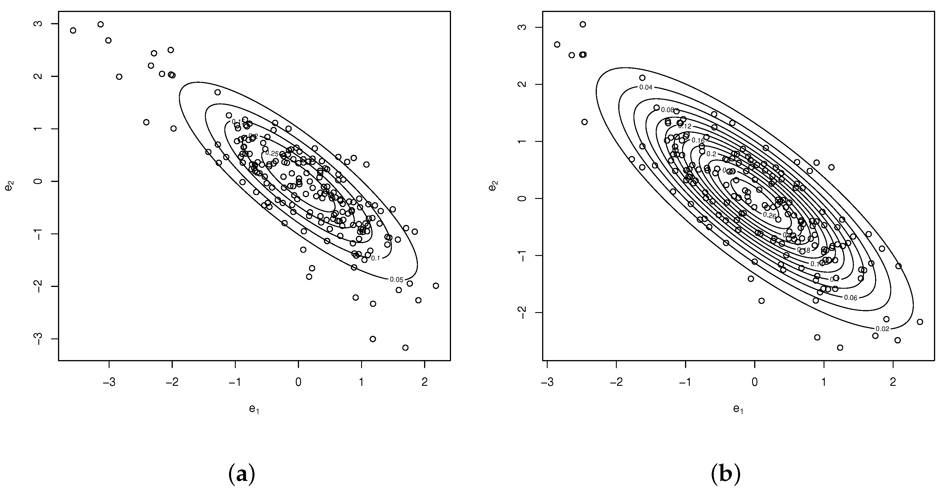
), respectively; that is, the assumption of multivariate normality is rejected. The contour plot for the BN distribution is presented in Figure 4a. Calculating the Mahalanobis distance, we find that the observations {11, 13, 14, 27, 142, 143, 192, 193, 195} are considered outliers. Eliminating this set of observations, we estimate the parameters of the model, obtaining now the ML estimates (standard errors between parentheses) presented in Table 3.
The Shapiro–Wilk and Doornik–Hansen bivariate normality tests for the vector ( e i 1 , e i 2 ) return the values 0.9914 (p- value > 0.05 ) and 3.9346 (p- value > 0.05 ), respectively; that is, the assumption of multivariate normality is not rejected.

8. Concluding Remarks

The statistical modeling of proportions, rates, or indices data is a very common activity in many areas of knowledge, such as medicine, economy, engineering, or social sciences. Although there are some proposals for modeling this type of data, in the statistical literature there are few alternatives capable of jointly modeling two or more variables of this type, even less so with the possibility of considering covariates to explain the variability of the responses.
In this work, from a transformation applied to a vector with a bivariate unit-Birnbaum–Saunders distribution, we have obtained a new bivariate distribution which is called the bivariate unit-sinh-normal (BVSHN) distribution. The new distribution is an absolutely continuous distribution and is useful for modeling data as described previously, that is, responses over the region ( 0 , 1 ) × ( 0 , 1 ) jointly. Based on the introduced proposal, the extension to the case of the regression model for bounded responses in ( 0 , 1 ) × ( 0 , 1 ) was proposed, which was called the BVUSHN regression model. In particular, for the introduced distribution, the joint probability density function and joint cumulative distribution were specified. Conditional distributions and the joint survival function were also presented. The estimation of the model parameters was carried out from a classical approach by using the maximum likelihood method together with the two-step method proposed by Joe [39]. A Monte Carlo simulation study was also carried out to evaluate the benefits and limitations of the introduced proposals, yielding good asymptotic results for the parameter estimators.
The BVUSHN distribution and the BVUSHN regression model showed great flexibility in fitting data to ( 0 , 1 ) , which is frequently encountered in many practical scenarios. The results obtained in the two applications showed better results than other existing methodologies in the literature, and therefore we conclude that our proposals are viable alternatives in the field of distribution theory and regression models.
Future works based on the results of this proposal could contemplate the extension to the case of more than two response variables and make inferences in the models considering a Bayesian perspective.

Author Contributions

Conceptualization, G.M.-F.; Data curation, A.J.L. and G.M.-A.; Formal analysis, G.M.-F., A.J.L. and G.M.-A.; Funding acquisition, R.T.-F.; Investigation, G.M.-F., A.J.L. and G.M.-A.; Methodology, G.M.-F., A.J.L. and G.M.-A.; Project administration, G.M.-F.; Resources, G.M.-A. and R.T.-F.; Software, G.M.-F. and A.J.L.; Supervision, G.M.-F., A.J.L. and G.M.-A.; Validation, A.J.L. and G.M.-A.; Visualization, G.M.-F. and A.J.L.; Writing—original draft, G.M.-F., A.J.L., G.M.-A. and R.T.-F.; Writing—review & editing, G.M.-F., A.J.L. and R.T.-F. All authors have read and agreed to the published version of the manuscript.

Funding

The research of G. Martínez-Flórez and R. Tovar-Falón was supported by project: Resolución de Problemas de Situaciones Reales Usando Análisis Estadístico a través del Modelamiento Multidimensional de Tasas y Proporciones; Esquemas de Monitoreamiento para Datos Asimétricos no Normales y una Estrategia Didáctica para el Desarrollo del Pensamiento Lógico-Matemático. Universidad de Córdoba, Colombia, Acta de Compromiso Número FCB-05-19.

Institutional Review Board Statement

Not applicable.

Informed Consent Statement

Not applicable.

Data Availability Statement

Details about the available data are given in Section 7.

Acknowledgments

G. Martínez-Flórez and R. Tovar-Falón acknowledge the support given by Universidad de Córdoba, Montería, Colombia.

Conflicts of Interest

The authors declare no conflict of interest.

Appendix A. Tables of Simulations

This section presents the results of the simulation study described in Section 6.
Table A1. Asymptotic behavior of the MLE for the BVSHN regression model with parameter vector θ = ( α 1 , β 1 , σ 1 , α 2 , β 2 , σ 2 , ρ ) . Simulation scenario 1.
ρ = 0.25 ρ = 0.50 ρ = 0.75
n EstimatesMeanAVBRMSEMeanAVBRMSEMeanAVBRMSE
α ^ 1 2.85471.35475.06992.98251.48256.57732.79541.29544.9636
β ^ 10 0.26430.01430.05880.26510.01510.05310.26310.01310.0538
β ^ 11 0.71130.03870.17530.70720.04280.16100.71460.03540.1597
σ ^ 1 0.82880.17120.31390.84690.15310.36780.83060.16940.2754
30 α ^ 2 4.15171.65179.24414.18881.68889.24864.21041.710410.1232
β ^ 20 −0.49630.00370.0900−0.48290.01710.0854−0.49010.00990.0924
β ^ 21 0.23500.01500.27290.20820.04180.26280.21690.03310.2786
σ ^ 2 0.87540.12460.17460.88410.11590.21150.87540.12460.2247
ρ ^ 0.24570.00430.03340.49440.00560.02220.74610.00390.0088
α ^ 1 2.17750.67751.72762.20950.70951.73572.07790.57791.4032
β ^ 10 0.26070.01070.02880.26440.01440.03140.25780.00780.0264
β ^ 11 0.71200.03800.08330.70820.04180.09480.71980.03020.0793
σ ^ 1 0.91440.08560.24690.90370.09630.33080.94260.05740.2417
50 α ^ 2 3.31820.81823.00383.36410.86413.17343.29900.79902.3721
β ^ 20 −0.49710.00290.0467−0.49010.00990.0461−0.49350.00650.0476
β ^ 21 0.26260.01260.13410.21680.03320.14760.22360.02640.1482
σ ^ 2 0.94120.05880.12040.93590.06410.12630.90970.09030.0834
ρ ^ 0.24580.00420.02040.49460.00540.01250.74640.00360.0047
α ^ 1 1.83090.33090.52971.78450.28450.49541.77430.27430.4677
β ^ 10 0.25920.00920.01390.26420.01420.01400.25740.00740.0127
β ^ 11 0.71360.03640.03970.71060.03940.04130.72090.02910.0383
σ ^ 1 0.94120.05880.11470.96190.03810.22670.96130.03870.1071
100 α ^ 2 2.80440.30440.82652.84060.34060.87152.85150.35150.8446
β ^ 20 −0.49720.00280.0223−0.49610.00390.0203−0.49360.00640.0193
β ^ 21 0.23910.01090.06570.23150.01850.06050.22430.02570.0612
σ ^ 2 0.97530.02470.04050.96480.03520.03780.95970.04030.0408
ρ ^ 0.24620.00380.00910.49470.00530.00580.74650.00350.0021
α ^ 1 1.67030.17030.21981.65470.15470.19251.64700.14700.1822
β ^ 10 0.25640.00640.00640.26350.01350.00670.25680.00680.0063
β ^ 11 0.71660.03340.02020.71610.03390.01950.72360.02640.0191
σ ^ 1 0.95680.04320.04540.96280.03720.05930.96160.03840.0397
200 α ^ 2 2.65810.15810.32602.67040.17040.35132.64780.14780.2894
β ^ 20 −0.50160.00160.0092−0.49620.00380.0097−0.49460.00540.0092
β ^ 21 0.24090.00910.02970.23200.01800.02930.22530.02470.0279
σ ^ 2 0.98060.01940.01690.97900.02100.01670.97790.02210.0145
ρ ^ 0.24690.00310.00440.49480.00520.00280.74760.00240.0010
α ^ 1 1.59920.09920.07271.58990.08990.06771.58750.08750.0602
β ^ 10 0.25580.00580.00300.25810.00810.00270.25630.00630.0023
β ^ 11 0.72150.02850.00900.71650.03350.00850.72620.02380.0074
σ ^ 1 0.95780.04220.01520.96450.03550.01440.96270.03730.0126
500 α ^ 2 2.56540.06540.12942.55180.05180.11702.55470.05470.0966
β ^ 20 −0.49920.00080.0039−0.49620.00380.0036−0.49580.00420.0035
β ^ 21 0.24330.00670.01170.23260.01740.01140.22820.02180.0109
σ ^ 2 0.99350.00650.00720.99360.00640.00660.98880.01120.0053
ρ ^ 0.25230.00230.00180.50480.00480.00120.74890.00110.0004
α ^ 1 1.59000.09000.03921.57490.07490.03531.56740.06740.0318
β ^ 10 0.25420.00420.00140.25790.00790.00140.25370.00370.0011
β ^ 11 0.72650.02350.00500.71680.03320.00460.72850.02150.0038
σ ^ 1 0.96040.03960.00830.98180.01820.00770.96630.03370.0070
1000 α ^ 2 2.53900.03900.05272.52700.02700.05582.53300.03300.0435
β ^ 20 −0.50050.00050.0019−0.49960.00040.0019−0.50340.00340.0018
β ^ 21 0.25360.00360.00580.23870.01130.00570.23420.01580.0058
σ ^ 2 0.99430.00570.00300.99560.00440.00330.99080.00920.0024
ρ ^ 0.24860.00140.00090.49840.00160.00060.75000.00000.0002
Table A2. Asymptotic behavior of the MLE for the BVSHN regression model with parameter vector θ = ( α 1 , β 1 , σ 1 , α 2 , β 2 , σ 2 , ρ ) . Simulation scenario 2.
ρ = 0.25 ρ = 0.75
n EstimatesMeanAVBRMSEMeanAVBRMSE
α ^ 1 3.63371.63377.81273.60731.60736.9422
β ^ 10 0.27110.02110.07310.27400.02400.0706
β ^ 11 0.62630.12370.22980.62580.12420.2177
σ ^ 1 0.82030.17970.22960.81340.18660.2227
30 α ^ 2 2.07791.57794.83522.06821.56824.8138
β ^ 20 −0.50490.00490.0103−0.50600.00600.0093
β ^ 21 0.26350.01350.03310.28090.03090.0281
σ ^ 2 0.48000.52000.50770.49410.50590.5365
ρ ^ −0.24140.00860.0353−0.73720.01280.0097
α ^ 1 2.95690.95692.78292.85850.85852.3274
β ^ 10 0.27040.02040.03860.27270.02270.0381
β ^ 11 0.62940.12060.12300.63520.11480.1233
σ ^ 1 0.85610.14390.15280.85410.14590.1058
50 α ^ 2 1.36170.86171.47471.26610.76611.1609
β ^ 20 −0.50440.00440.0048−0.50570.00570.0046
β ^ 21 0.26220.01220.01490.27680.02680.0139
σ ^ 2 0.60780.39220.44270.62160.37840.4356
ρ ^ −0.24180.00820.0200−0.73720.01280.0044
α ^ 1 2.48040.48040.83742.41970.41970.6970
β ^ 10 0.26950.01950.01900.26780.01780.0182
β ^ 11 0.62970.12030.06430.63560.11440.0656
σ ^ 1 0.88630.11370.05020.89330.10670.0416
100 α ^ 2 0.93430.43430.41760.91800.41800.3931
β ^ 20 −0.50330.00330.0022−0.50400.00400.0021
β ^ 21 0.26210.01210.00680.27570.02570.0069
σ ^ 2 0.74640.25360.32410.75760.24240.3472
ρ ^ −0.24240.00760.0105−0.73940.01060.0022
α ^ 1 2.28020.28020.35192.28940.28940.3037
β ^ 10 0.26770.01770.00870.26650.01650.0086
β ^ 11 0.63450.11550.04040.63810.11190.0377
σ ^ 1 0.91400.08600.02890.91010.08990.0239
200 α ^ 2 0.72950.22950.15670.71870.21870.1455
β ^ 20 −0.50180.00180.0012−0.50330.00330.0011
β ^ 21 0.26060.01060.00350.27560.02560.0039
σ ^ 2 0.88440.11560.31660.86160.13840.2346
ρ ^ −0.24390.00610.0044−0.73960.01040.0011
α ^ 1 2.22050.22050.14282.17410.17410.1050
β ^ 10 0.26660.01660.00380.26530.01530.0034
β ^ 11 0.63920.11080.02380.65270.09730.0216
σ ^ 1 0.91550.08450.01420.92550.07450.0113
500 α ^ 2 0.60640.10640.06190.59090.09090.0546
β ^ 20 −0.50120.00120.0005−0.50240.00240.0004
β ^ 21 0.25890.00890.00150.27510.02510.0019
σ ^ 2 1.05950.05950.25080.98630.01370.2383
ρ ^ −0.24500.00500.0018−0.74280.00720.0005
α ^ 1 2.19770.19770.08462.14320.14320.0556
β ^ 10 0.26460.01460.00210.25830.00830.0018
β ^ 11 0.64830.10170.01980.65280.09720.0175
σ ^ 1 0.91630.08370.01040.93040.06960.0076
1000 α ^ 2 0.54170.04170.03300.54280.04280.0288
β ^ 20 −0.50010.00010.0002−0.50110.00110.0002
β ^ 21 0.25740.00740.00080.26980.01980.0013
σ ^ 2 0.98700.01300.23351.01310.01310.1658
ρ ^ −0.24530.00470.0010−0.74500.00500.0004
Table A3. Asymptotic behavior of the MLE for the BVSHN regression model with parameter vector θ = ( α 1 , β 1 , σ 1 , α 2 , β 2 , σ 2 , ρ ) . Simulation scenario 3.
ρ = 0.50 ρ = 0.50
n EstimatesMeanAVBRMSEMeanAVBRMSE
α ^ 1 2.20251.45254.84263.14972.14978.8825
β ^ 10 1.50160.00160.00511.16110.33890.1740
β ^ 11 −0.50830.00830.0157−0.30150.19850.2205
σ ^ 1 0.36210.13790.27770.87010.87991.1743
30 α ^ 2 2.45971.45975.10214.67331.673314.0574
β ^ 20 −1.23970.01030.0747−1.46250.21250.2703
β ^ 21 0.73460.01540.21650.37380.12380.6797
σ ^ 2 1.07210.42790.73491.31570.18430.3368
ρ ^ −0.50340.00340.02220.48330.01670.0305
α ^ 1 1.45890.70891.37582.22091.22093.1101
β ^ 10 1.50160.00160.00321.16330.33670.1539
β ^ 11 −0.49590.00410.0087−0.30190.19810.1472
σ ^ 1 0.45270.04730.22131.07100.67901.0229
50 α ^ 2 1.78640.78641.66333.78230.78233.5003
β ^ 20 −1.25410.00410.0391−1.44900.19900.1574
β ^ 21 0.73990.01010.12470.36550.11550.3518
σ ^ 2 1.23420.26580.60931.39690.10310.1848
ρ ^ −0.50200.00200.01280.49400.00600.0197
α ^ 1 1.07000.32000.41331.67800.67801.1032
β ^ 10 1.50130.00130.00301.17410.32590.1244
β ^ 11 −0.50280.00280.0036−0.30360.19640.0917
σ ^ 1 0.54050.04050.22181.21430.53570.7571
100 α ^ 2 1.30410.30410.42073.30020.30021.0830
β ^ 20 −1.24600.00400.0209−1.43910.18910.0881
β ^ 21 0.75550.00550.05920.36160.11160.1575
σ ^ 2 1.44730.05270.48271.43760.06240.0812
ρ ^ −0.50050.00050.00570.49440.00560.0127
α ^ 1 0.87530.12530.13901.44080.44080.5224
β ^ 10 1.49890.00110.00271.18340.31660.1095
β ^ 11 −0.50220.00220.0020−0.31990.18010.0580
σ ^ 1 0.53600.03600.12211.22200.52800.5589
200 α ^ 2 1.12270.12270.16242.92380.07620.3892
β ^ 20 −1.24850.00150.0088−1.43180.18180.0560
β ^ 21 0.75360.00360.02690.34670.09670.0770
σ ^ 2 1.52440.02440.31291.47150.02850.0321
ρ ^ −0.50050.00050.00290.49470.00530.0089
α ^ 1 0.78720.03720.05871.32710.32710.2423
β ^ 10 1.50030.00030.00161.19140.30860.0991
β ^ 11 −0.50050.00050.0010−0.32870.17130.0393
σ ^ 1 0.52400.02400.08061.24610.50390.3871
500 α ^ 2 1.03940.03940.05443.04490.04490.1462
β ^ 20 −1.24950.00050.0048−1.42720.17720.0426
β ^ 21 0.74750.00250.01030.34310.09310.0346
σ ^ 2 1.51780.01780.11121.47390.02610.0118
ρ ^ −0.50040.00040.00120.49500.00500.0070
α ^ 1 0.75590.00590.02751.29690.29690.1549
β ^ 10 1.50020.00020.00091.19190.30810.0967
β ^ 11 −0.50030.00030.0007−0.32920.17080.0340
σ ^ 1 0.51730.01730.02261.26780.48220.3275
1000 α ^ 2 1.01080.01080.02472.98110.01890.0670
β ^ 20 −1.25010.00010.0017−1.42590.17590.0363
β ^ 21 0.75070.00070.00350.33650.08650.0220
σ ^ 2 1.51630.01630.04871.48600.01400.0052
ρ ^ −0.49990.00010.00050.49810.00190.0064

References

  1. Birnbaum, Z.W.; Saunders, S.C. A new family of life distributions. J. Appl. Probab. 1969, 6, 319–327. [Google Scholar] [CrossRef]
  2. Birnbaum, Z.W.; Saunders, S.C. Estimation for a family of life distributions with applications to fatigue. J. Appl. Probab. 1969, 6, 328–347. [Google Scholar] [CrossRef]
  3. Díaz-García, J.A.; Leiva-Sánchez, V. A new family of life distributions based on the elliptically contoured distributions. J. Statist. Plann. Inference 2005, 128, 445–457. [Google Scholar] [CrossRef]
  4. Vilca-Labra, F.; Leiva-Sánchez, V. A new fatigue life model based on the family of skew-elliptical distributions. Commun. Stat.-Theory Methods 2006, 35, 229–244. [Google Scholar] [CrossRef]
  5. Gómez, H.W.; Olivares-Pacheco, J.F.; Bolfarine, H. An extension of the generalized Birnbaun-Saunders distribution. Stat. Probab. Lett. 2009, 79, 331–338. [Google Scholar] [CrossRef]
  6. Castillo, N.O.; Gómez, H.W.; Bolfarine, H. Epsilon Birnbaum–Saunders distribution family: Properties and inference. Stat. Pap. 2011, 52, 871–883. [Google Scholar] [CrossRef]
  7. Martínez-Flórez, G.; Bolfarine, H.; Gómez, H.W. An alpha-power extension for the Birnbaum–Saunders distribution. Stat. J. Theor. Appl. Stat. 2014, 48, 896–912. [Google Scholar] [CrossRef]
  8. Martínez-Flórez, G.; Bolfarine, H.; Gómez, H.W. The Log-Linear Birnbaum-Saunders Power Model. Methodol. Comput. Appl. Probab. 2017, 19, 913–933. [Google Scholar] [CrossRef]
  9. Moreno-Arenas, G.; Martínez-Flórez, G.; Bolfarine, H. Power Birnbaum-Saunders Student t distribution. Rev. Integr. 2017, 35, 51–70. [Google Scholar]
  10. Balakrishnan, N.; Kundu, D. Birnbaum-Saunders distribution: A review of models, analysis, and applications. Mathematics 2018, 35, 1–41. [Google Scholar] [CrossRef]
  11. Athayde, E.; Azevedo, A.; Barros, M.; Leiva, V. Failure rate of Birnbaum–Saunders distributions: Shape, change-point, estimation and robustness. Braz. J. Probab. Stat. 2019, 33, 301–328. [Google Scholar] [CrossRef] [Green Version]
  12. Arrué, J.; Arellano, R.; Gomez, H.W.; Leiva, V. On a new type of Birnbaum-Saunders models and its inference and application to fatigue data. J. Appl. Stat. 2020, 47, 2690–2710. [Google Scholar] [CrossRef]
  13. Reyes, R.; Arruúe, J.; Víctor Leiva, V.; Martin-Barreiro, C. A new Birnbaum–Saunders distribution and its mathematical features applied to bimodal real-world data from environment and medicine. Mathematics 2021, 9, 1891. [Google Scholar] [CrossRef]
  14. Mazucheli, J.; Menezes, A.; Dey, S. The unit-Birnbaum-Saunders distribution with applications. Chil. J. Stat. 2018, 9, 47–57. [Google Scholar]
  15. Rieck, J.R.; Nedelman, J.R. A log-linear model for the Birnbaum-Saunders distribution. Technometrics 1991, 33, 51–60. [Google Scholar]
  16. Barros, M.; Paula, G.A.; Leiva, V. A new class of survival regression models with heavy-tailed errors: Robustness and diagnostics. Lifetime Data Anal. 2008, 14, 316–332. [Google Scholar] [CrossRef]
  17. Leiva, V.; Vilca, F.; Balakrishnan, N.; Sanhueza, A. A skewed sinh-normal distribution and its properties and application to air pollution. Commun. Stat. Theory Methods 2010, 39, 426–443. [Google Scholar] [CrossRef]
  18. Lemonte, A. A log-Birnbaum-Saunders Regression Model with Asymmetric Errors. J. Stat. Comput. Simul. 2012, 82, 1775–1787. [Google Scholar] [CrossRef]
  19. Santana, L.; Vilca, F.; Leiva, V. Influence analysis in skew-Birnbaum-Saunders regression models and applications. J. Appl. Stat 2011, 38, 1633–1649. [Google Scholar] [CrossRef]
  20. Kundu, D.; Balakrishnan, N.; Jamalizadeh, A. Bivariate Birnbaum-Saunders distribution and associated inference. J. Multivar. Anal. 2010, 101, 113–125. [Google Scholar] [CrossRef]
  21. Lemonte, A.J.; Martínez-Flórez, G.; Moreno-Arenas, G. Multivariate Birnbaum–Saunders distribution: Properties and associated inference. J. Stat. Comput. Simul. 2015, 85, 374–392. [Google Scholar] [CrossRef]
  22. Lemonte, A.J. Multivariate Birnbaum–Saunders regression model. J. Stat. Comput. Simul. 2013, 83, 2244–2257. [Google Scholar] [CrossRef]
  23. Kundu, D. Bivariate sinh-normal distribution and a related model. Braz. J. Probab. Stat. 2015, 29, 590–607. [Google Scholar] [CrossRef]
  24. Martínez-Flórez, G.; Azevedo-Farias, R.B.; Moreno-Arenas, G. Multivariate log-Birnbaum–Saunders regression models. Commun. Stat.-Theory Methods 2017, 46, 10166–10178. [Google Scholar] [CrossRef]
  25. Martínez-Flórez, G.; Azevedo-Farias, R.B.; Tovar-Falón, R. An Exponentiated Multivariate Extension for the Birnbaum-Saunders Log-Linear Model. Mathematics 2022, 10, 1299. [Google Scholar] [CrossRef]
  26. Paolino, P. Maximum likelihood estimation of models with beta-distributed dependent variables. Political Anal. 2001, 9, 325–346. [Google Scholar] [CrossRef]
  27. Cribari-Neto, F.; Vasconcellos, K.L.P. Nearly unbiased maximum likelihood estimation for the beta distribution. J. Stat. Comput. Simul. 2002, 72, 107–118. [Google Scholar] [CrossRef]
  28. Kieschnick, R.; McCullough, B.D. Regression analysis of variates observed on (0, 1): Percentages, proportions and fractions. Stat. Model. 2003, 3, 193–213. [Google Scholar] [CrossRef]
  29. Ferrari, S.; Cribari-Neto, F. Beta regression for modelling rates and proportions. J. Appl. Stat. 2004, 31, 799–815. [Google Scholar] [CrossRef]
  30. Vasconcellos, K.L.P.; Cribari-Neto, F. Improved maximum likelihood estimation in a new class of beta regression models. Braz. J. Probab. Stat. 2005, 19, 13–31. [Google Scholar]
  31. Branscum, A.J.; Johnson, W.O.; Thurmond, M.C. Bayesian beta regression: Applications to household expenditure data and genetic distance between foot-and-mouth diseases viruses. Aust. N. Z. J. Stat. 2007, 49, 287–301. [Google Scholar] [CrossRef]
  32. Bayes, C.L.; Bazan, J.L.; García, C. A new robust regression model for proportions. Bayesian Anal. 2012, 7, 841–866. [Google Scholar] [CrossRef]
  33. Ospina, R.; Ferrari, S.L.P. Inflated beta distribution. Stat. Pap. 2010, 51, 111–126. [Google Scholar] [CrossRef]
  34. Ospina, R.; Ferrari, S.L.P. A general class of zero-or-one inflated beta regression models. Comput. Stat. Data Anal. 2012, 56, 1609–1623. [Google Scholar] [CrossRef] [Green Version]
  35. Martínez-Flórez, G.; Bolfarine, H.; Gómez, H.W. Doubly censored power-normal regression models with inflation. Test 2014, 24, 265–286. [Google Scholar] [CrossRef]
  36. Martínez-Flórez, G.; Bolfarine, H.; Gómez, H.W. Power-models for proportions with zero/one excess. Appl. Math. Inf. Sci. 2018, 24, 293–303. [Google Scholar] [CrossRef]
  37. Martínez-Flórez, G.; Tovar-Falón, R.; Barrera-Causil, C. Inflated Unit-Birnbaum-Saunders Distribution. Mathematics 2022, 10, 667. [Google Scholar] [CrossRef]
  38. Marshall, A.W. Some comments on the hazard gradient. Stoch. Process. Their Appl. 1975, 3, 293–300. [Google Scholar] [CrossRef]
  39. Joe, H. Asymptotic efficiency of the two-stage estimation method for copula-based models. J. Multivar. Anal. 2005, 94, 401–419. [Google Scholar] [CrossRef]
  40. R Development Core Team. R: A Language and Environment for Statistical Computing; R Foundation for Statistical Computing: Vienna, Austria, 2021; Available online: http://www.R-project.org (accessed on 28 February 2022).
  41. Meintanis, S.G. Test of fit for Marshall-Olkin distributions with applications. J. Stat. Plan. Inference 2007, 137, 3954–3963. [Google Scholar] [CrossRef]
Figure 1. Asymptotic behavior of the MLE for the BVSHN regression model for scenario 1.
Mathematics 10 03125 g001aMathematics 10 03125 g001bMathematics 10 03125 g001c
Figure 2. Asymptotic behavior of the MLE for the BVSHN regression model for scenario 2.
Mathematics 10 03125 g002aMathematics 10 03125 g002bMathematics 10 03125 g002c
Figure 3. Contour plots of bivariate distributions: (a) BVLN, (b) BVBS, and (c) BVUBS.
Mathematics 10 03125 g003
Figure 4. Contour plot of the bivariate vector ( e i 1 , e i 2 ) : (a) with outliers and (b) without outliers.
Mathematics 10 03125 g004
Table 1. Estimation of the parameters with their standard errors for the BVBS, BVLN, and BVUBS distributions.
EstimatorBVBSBVLNBVUBS
α ^ 1 0.8305   ( 0.0971 ) 0.8236   ( 0.0962 )
α ^ 2 1.0659   ( 0.1253 ) 1.1160   ( 0.1301 )
β ^ 1 0.3204   ( 0.0402 ) 0.6840   ( 0.0846 )
β ^ 2 0.2209   ( 0.0339 ) 0.7786   ( 0.1218 )
μ ^ 1 0.9637   ( 0.1154 )
μ ^ 2 1.3233   ( 0.1556 )
σ ^ 1 0.7024   ( 0.0816 )
σ ^ 2 0.9469   ( 0.1100 )
ρ ^ 0.5558   ( 0.1152 ) 0.5066   ( 0.1221 ) 0.5966   ( 0.1065 )
AIC 15.7486 9.6148 11.8823
BIC 29.4732 25.3395 3.8277
Table 2. Estimation of the parameters with their standard errors for the BVUSHN regression model.
EstimatorBVUBS
α ^ 1 0.0173   ( 0.0051 )
α ^ 2 0.1786   ( 0.0952 )
β ^ 10 3.9374   ( 0.8521 )
β ^ 11 0.5342   ( 0.0420 )
β ^ 12 0.9140   ( 0.1979 )
β ^ 20 6.9501   ( 6.4588 )
β ^ 21 3.5038   ( 0.3266 )
β ^ 22 2.3048   ( 1.5009 )
σ ^ 1 6.7323   ( 2.0491 )
σ ^ 2 5.6380   ( 2.9657 )
ρ ^ 0.8435   ( 0.0251 )
Table 3. Estimation of the parameters with their standard errors for the BVUSHN regression model without outliers.
EstimatorBVUBS
α ^ 1 0.0145   ( 0.0038 )
α ^ 2 0.1412   ( 0.0554 )
β ^ 10 3.8892   ( 0.6937 )
β ^ 11 0.5408   ( 0.0339 )
β ^ 12 0.9046   ( 0.1611 )
β ^ 20 6.9470   ( 5.5195 )
β ^ 21 3.6462   ( 0.2752 )
β ^ 22 2.3220   ( 1.2821 )
σ ^ 1 6.8814   ( 1.9256 )
σ ^ 2 6.0481   ( 2.3610 )
ρ ^ 0.8172   ( 0.0274 )
Publisher’s Note: MDPI stays neutral with regard to jurisdictional claims in published maps and institutional affiliations.

