Fast Image Restoration Method Based on the L₀, L₁, and L₂ Gradient Minimization

Abstract

In this paper, we propose a novel image denoising method by coupling with $L_0$, $L_1$ and $L_2$ gradient minimization. Our proposed method smoothes the gradient difference between image pixels and noise pixels and sharpens the edges by increasing the steepness of transition. We focus on global noise processing rather than local features and adaptively process noise signals with different characteristics. Based on the half-quadratic splitting method, we perform a smoothing step realized by a Poisson approach and two edge-preserving steps through an optimization formulation. This iterative method is fast, simple, and easy to implement. The proposed numerical scheme can be performed to a discrete cosine transform implementation, which can be applied with parallel GPUs computing in a straightforward manner. Various tests are presented, including both qualitative and quantitative tests, to demonstrate that the proposed method is efficient and robust for producing image processing results with good quality.

1. Introduction

Image restoration is the process of estimating the clean image from the corrupt/noisy image. Up to now, a great number of models have been proposed to console the image restoration problem. Bilateral filtering with the explicit kernel is widely used for its effectiveness in removing noise-like structures [1]. The output of this method is a weighted average of the nearby pixels at the specific pixel, where the weight combinators depend on the intensity similarities based on the guidance image. The median filter [2] is a well-known edge-aware operator, which is a special case of local histogram filters [3]. He et al. proposed a novel explicit image filter called guided filter, which computes the filtering output by considering the content of a guidance image [4]. Edge-preserving smoothing can be achieved by other local filtering, for example, targeted image denoising filtering (TID) [5], transform-domain collaborative filtering(BM3D) [6], transform-domain collaborative filtering with shape-adaptive principal component analysis(BM3D-PCA) [7] and principal component analysis with local pixel grouping(LPG-PCA) [8]. Chambolle and Pock [9] proposed a first-order primal-dual algorithm for the non-smooth convex optimization problems with a convergence rate of $O(1/N)$. He and Yuan [10] focused on the convergence analysis and proposed a modified primal-dual algorithm for solving a saddle-point problem. Chen and Xu [11] proposed an iterative algorithm for sparse view X-ray tomography to avoid solving the large scale. They provided the rigorous proofs of the convergence for the aforementioned problems.

Another type of image regularization is total variation, which has achieved great success in image restoration and sharpening edges [12]. Chan and Shen [13] repaired the images by minimizing the image gradient based on the curvature-driven diffusions. To solve image inpainting and image reduces problems, Esedoḡlu and Shen introduced the Mumford–Shah–Euler model [14] based on the Mumford–Shah image segmentation model [15], Li et al. concerned with fast domain decomposition methods for solving the total variation minimization problems in image processing [16]. In [17], the authors proposed the group sparsity-based algorithm for nuclear radiation-contaminated video restoration. Liu presented a novel nonconvex extension model that closely incorporates the advantages of total generalized variation and edge-enhancing nonconvex penalties [18]. Bertozzi et al. [19,20] introduced a well-known inpainting method with the modified Cahn–Hilliard equation [21]. By using the Allen–Cahn equation [22], which describes the motion of mean curvature flow [23,24], Li et al. extended Chan and Shen’s model [12] and proposed the fast image inpainting method with the efficient hybrid numerical solver [25,26].

The existing diffusion methods used the $L_1$-norm or $L_2$-norm in their proposed energy term and obtained the clean images by minimizing it to convergence. However, these methods suffer from a tendency of over-smooth on the processed image data due to the property of soft-thresholding. In order to sharpen the edges during the noise reduction, a novel fast and accurate method based on the $L_0$ gradient minimization [27] has been proposed to measure the sparsity of the solution with sharper edges. Some methods treat the image noises as signal type noise [28], such as speckle noise, pepper noise, and Gaussian noise. True image noise is much different to single noise, but is a mixture type noise. In this paper, we will propose a new image restoration method by coupling with $L_0$, $L_1$, and $L_2$ gradient minimization. The proposed method can be solved by the half-quadratic splitting method. We decoupled the iterations over the smoothing step and performed a Poisson approach after the alternating reformulation. Two edge-preserving steps have been used through the optimizing process to sharpen the edge of the target. The proposed iterative method is efficient and easy to implement. The main advantage of the proposed method can be summarized as follows: (i) This method transforms the problem of denoising to the optimization problem in which the clear image can be obtained by the iterative methods. (ii) The processing of noise reduction computation is based on the pixel information of the single image, which does not require a lot of training cost for the same type of images to obtain the desired accuracy. (iii) To the best of our knowledge, this is the first investigation on the combination of the hard- and soft-thresholding, which can balance the competitive advantage with proper parameter combinators. Several numerical tests will be presented to demonstrate the robustness and efficiency of our method.

The outline of this paper is as follows. The governing equations for the image restoration method are illustrated in Section 2. The proposed operator splitting algorithm is described in Section 3. The computational examples have been presented in Section 4 to demonstrate the efficiency and robustness of our proposed method. In Section 5, we drew the conclusions.

2. Proposed Image Restoration Method

For a 2D image representation, we combine the following $L_0$, $L_1$, and $L_2$ norm with gradient regularization version:

$$\underset{\varphi }{min}{\int }_{\mathsf{\Omega }}\left({\alpha \left|\right|\nabla \varphi \left(\mathbf{x}\right)\left|\right|}_0+{\beta \left|\right|\nabla \varphi \left(\mathbf{x}\right)\left|\right|}_1+{(1-\alpha -\beta )\left|\right|\nabla \varphi \left(\mathbf{x}\right)\left|\right|}_2^2+\lambda {(\varphi \left(\mathbf{x}\right)-I\left(\mathbf{x}\right))}^2\right)d\mathbf{x}$$

(1)

where $\mathbf{x}=(x,y)$, $f\left(\mathbf{x}\right)$ is a given image in a domain $\mathsf{\Omega }\subset {\mathbb{R}}^2$. The fidelity term $\lambda {(\varphi \left(\mathbf{x}\right)-I\left(\mathbf{x}\right))}^2$ is used for the detection of similarity between the processed image $\varphi$ and the given image I in $\mathsf{\Omega }$. In Equation (1), $\left|\right|·{\left|\right|}_0$, $\left|\right|·{\left|\right|}_1$, and $\left|\right|·{\left|\right|}_2$ are the $L_0$, $L_1$, and $L_2$ norms, respectively. Let us briefly review the definition of $L_0$-norm: if $\varphi =0$, then ${\left|\right|\varphi \left|\right|}_0=0$. Otherwise, ${\left|\right|\varphi \left|\right|}_0=1$. Therefore the term ${\left|\right|\nabla \varphi \left(\mathbf{x}\right)\left|\right|}_{\mathbf{0}}$ can reduce the noises and make edges sharpen. The minimization problem (1) is difficult to optimize directly due to the combinatorial nature of $L_0$, $L_1$, and $L_2$ minimization. Recently, a scalable algorithm was proposed for image processing [27,29] and surface smoothing [30,31] by considering the $L_0$ norm gradient optimization. Our work extends the $L_0$, $L_1$, and $L_2$ minimizations concept to image restoration. Let us provide the following Theorem:

Theorem 1.

By introducing a set of auxiliary variables $\psi =({\psi }^x,{\psi }^y)$ and $\phi =({\phi }^x,{\phi }^y)$, the minimization problem (1) is equivalent minimize the following equation:

$$\begin{array}{c}\hfill \begin{array}{cc}\hfill \underset{\varphi ,\psi ,\phi }{min}{\int }_{\mathsf{\Omega }}({\alpha \left|\right|\psi \left(\mathbf{x}\right)\left|\right|}_0+{\beta \left|\right|\phi \left(\mathbf{x}\right)\left|\right|}_1& +{(1-\alpha -\beta )\left|\right|\nabla \varphi \left(\mathbf{x}\right)\left|\right|}_2^2+\lambda {(\varphi \left(\mathbf{x}\right)-I\left(\mathbf{x}\right))}^2\hfill \\ & +\gamma \left|\right|\nabla \varphi \left(\mathbf{x}\right)-{\psi \left(\mathbf{x}\right)\left|\right|}_2^2+\zeta \left|\right|\nabla \varphi \left(\mathbf{x}\right)-{\phi \left(\mathbf{x}\right)\left|\right|}_2^2)d\mathbf{x}.\hfill \end{array}\end{array}$$

(2)

Here, γ and ζ are two weight parameters directly controlling the similarity between ψ, φ, and the gradient of ϕ.

Proof. 

The minimization problem (2) generally can be minimized by an alternating minimization method in the following manner:

(1)

for $\varphi$ and $\phi$ fixed,

$$\begin{array}{c}\hfill \underset{\psi }{min}{\int }_{\mathsf{\Omega }}\left({\alpha \left|\right|\psi \left|\right|}_0+\gamma \left|\right|\nabla \varphi -{\psi \left|\right|}_2^2\right)d\mathbf{x}.\end{array}$$

(3)

(2)

for $\varphi$ and $\psi$ fixed,

$$\begin{array}{c}\hfill \underset{\phi }{min}{\int }_{\mathsf{\Omega }}\left({\beta \left|\right|\phi \left|\right|}_1+\zeta \left|\right|\nabla \varphi -{\phi \left|\right|}_2^2\right)d\mathbf{x}.\end{array}$$

(4)

(3)

for $\phi$ and $\psi$ fixed,

$$\begin{array}{c}\hfill \underset{\varphi }{min}{\int }_{\mathsf{\Omega }}\left(\gamma \left|\right|\nabla \varphi -{\psi \left|\right|}_2^2+\zeta \left|\right|\nabla \varphi -{\phi \left|\right|}_2^2+{(1-\alpha -\beta )\left|\right|\nabla \varphi \left(\mathbf{x}\right)\left|\right|}_2^2+\lambda {(\varphi \left(\mathbf{x}\right)-I\left(\mathbf{x}\right))}^2\right)d\mathbf{x}\end{array}$$

(5)

In order to eventually force $\nabla \varphi$ to match $\psi$ and $\phi$, both of these optimizations alternate until convergence by increasing $\gamma$ and $\zeta$ at each iteration. The idea is summarized as:

Step 1. By considering the independence of $\mathbf{x}$, we can rewrite Equation (3) as

$$\begin{array}{c}\hfill {\int }_{\mathsf{\Omega }}\underset{\psi }{min}\left({\alpha \left|\right|\psi \left|\right|}_0+\gamma \left|\right|\nabla \varphi -{\psi \left|\right|}_2^2\right)d\mathbf{x}.\end{array}$$

(6)

Considering every point $\mathbf{x}\in \mathsf{\Omega }$, we need to minimize

$$\begin{array}{c}\hfill G_1\left(\psi \right)={\alpha \left|\right|\psi \left|\right|}_0+\gamma \left|\right|\nabla \varphi -{\psi \left|\right|}_2^2.\end{array}$$

(7)

Let us consider Equation (7): if $\gamma =0$, the minimum of $G_1$ can be obtained by setting $\psi =\nabla \varphi$; otherwise the relationship between ${\left|\right|\nabla \varphi \left(\mathbf{x}\right)\left|\right|}_2^2$ and $\gamma /\alpha$ should be analyzed. Let us summarized the relations as: When ${\left|\right|\nabla \varphi \left(\mathbf{x}\right)\left|\right|}_2^2\ge \alpha /\gamma$, we start splitting in the following two situations.

(1)

By considering $\psi \ne 0$, the minimal value $G_1^{*}$ can be obtained by setting $\nabla \varphi \left(\mathbf{x}\right)=\psi$ which can be shown as

$$G_1^{*}(\psi \ne 0)=\underset{\psi }{min}{G}_1(\psi \ne 0)={\alpha \left|\right|\psi \left|\right|}_0+\gamma \left|\right|\nabla \varphi -{\psi \left|\right|}_2^2=\alpha .$$

(8)

(2)

By considering that $\psi =0$, we can obtain

$$\begin{array}{cc}\hfill G_1^{*}(\psi =0)& =\underset{\psi }{min}{G}_1(\psi =0)\hfill \\ \hfill & ={\alpha \left|\right|\psi \left|\right|}_0+\gamma \left|\right|\nabla \varphi -{\psi \left|\right|}_2^2={\gamma \left|\right|\nabla \varphi \left|\right|}_2^2\ge \alpha =\underset{\psi }{min}{G}_1(\psi \ne 0).\hfill \end{array}$$

(9)

Therefore, we should only let $\nabla \varphi =\psi$ to obtain the minimum $G_1^{*}$. Therefore, by combining Equations (8) and (9), the minimum energy (6) is produced when $\nabla \varphi =\psi$. Hence, we can obtain the following condition:

$$\begin{array}{c}\hfill \psi =\left\{\begin{array}{cc}\nabla \varphi \hfill & {\mathrm{if}\left|\right|\nabla \varphi \left|\right|}_2^2\ge \alpha /\gamma ,\hfill \\ \mathbf{0}\hfill & \mathrm{otherwise}.\hfill \end{array}\right.\end{array}$$

(10)

Step 2. Let us rewrite Equation (4) by considering the independence of $\mathbf{x}$ as:

$$\begin{array}{c}\hfill {\int }_{\mathsf{\Omega }}\underset{\psi }{min}\left({\beta \left|\right|\phi \left|\right|}_1+\zeta \left|\right|\nabla \varphi -{\phi \left|\right|}_2^2\right)d\mathbf{x}.\end{array}$$

(11)

For every individual point x, we need to minimize

$$\begin{array}{c}\hfill G_2\left(\phi \right)={\alpha \left|\right|\phi \left|\right|}_1+\gamma \left|\right|\nabla \varphi -{\phi \left|\right|}_2^2=G_2^x\left({\phi }^x\right)+G_2^y\left({\phi }^y\right).\end{array}$$

(12)

Here, $\nabla \varphi =({\varphi }_x,{\varphi }_y)$ and $G_2^x\left({\phi }^x\right)=\alpha \left|{\phi }^x\right|+\gamma {({\varphi }_x-{\phi }^x)}^2$ and $G_2^y\left({\phi }^y\right)=\alpha \left|{\phi }^y\right|+\gamma {({\varphi }_y-{\phi }^y)}^2$. It is obvious that ${\phi }^x={\varphi }_x-\alpha \mathrm{sign}\left({\phi }^x\right)/\left(2\gamma \right)$ and ${\phi }^y={\varphi }_y-\alpha \mathrm{sign}\left({\phi }^y\right)/\left(2\gamma \right)$ are the minima points of $G_2^x\left({\phi }^x\right)$ and $G_2^y\left({\phi }^y\right)$, respectively. Here, $\mathrm{sign}\left(\right)$ is the sign function, which is defined as 1 for positive argument and -1 for negative argument. If ${\varphi }_x>\alpha /\left(2\gamma \right)$, then $G_2^x({\phi }^x={\varphi }_x-\alpha /\left(2\gamma \right))<\alpha {\left({\varphi }_x\right)}^2=G_2^x({\phi }^x=0)$. Therefore, ${\phi }^x={\varphi }_x-\alpha /\left(2\gamma \right)$ is the minimization of $G_2^x\left({\phi }^x\right)$. In the similar fashion, if ${\varphi }_x<-\alpha /\left(2\gamma \right)$, we should set ${\phi }^x={\varphi }_x+\alpha /\left(2\gamma \right)$ to minimize the $G_2^x\left({\phi }^x\right)$. It is obvious that if $|{\varphi }_x|<\alpha /\left(2\gamma \right)$, then ${\phi }^x=0$ is the minimization of $G_2^x\left({\phi }^x\right)$. In summary, we can obtain the following condition:

$$\begin{array}{c}\hfill {\phi }^x=\left\{\begin{array}{cc}{\varphi }_x+\alpha /\left(2\gamma \right)\hfill & \mathrm{if} {\varphi }_x<-\alpha /\left(2\gamma \right),\hfill \\ 0\hfill & \mathrm{if} \left|{\varphi }_x\right|<\alpha /\left(2\gamma \right),\hfill \\ {\varphi }_x-\alpha /\left(2\gamma \right)\hfill & \mathrm{if} {\varphi }_x>\alpha /\left(2\gamma \right),\hfill \end{array}\right.\mathrm{and} {\phi }^y=\left\{\begin{array}{cc}{\varphi }_y+\alpha /\left(2\gamma \right)\hfill & \mathrm{if} {\varphi }_y<-\alpha /\left(2\gamma \right),\hfill \\ 0\hfill & \mathrm{if} \left|{\varphi }_y\right|<\alpha /\left(2\gamma \right),\hfill \\ {\varphi }_y-\alpha /\left(2\gamma \right)\hfill & \mathrm{if} {\varphi }_y>\alpha /\left(2\gamma \right).\hfill \end{array}\right.\end{array}$$

(13)

Step 3. The expression (5) is quadratic in $\varphi$ and trivial to minimize. Following the Euler–Lagrange formulation, $\varphi$ minimizes Equation (5) as

$$\begin{array}{c}\hfill \gamma \nabla ·(\nabla \varphi -\psi )+\zeta \nabla ·(\nabla \varphi -\phi )+(1-\alpha -\beta )\Delta \varphi -\lambda (\varphi -I)=0.\end{array}$$

(14)

Therefore, in order to get the solution of the minimization problem (2), three optimizations (Equations (10), (13), and (14)) alternate until convergence by increasing $\gamma$ and $\zeta$ at each iteration. □

Some notations should be summarized as follows: (i) $\alpha$ and $\beta$ are the convex combinators for controlling the similarity between $\psi$ and $\phi$ with $\nabla \varphi$. Since the $L_0$-norm and $L_1-norm$ regularized optimization problem is know as computationally intractable, we use the equivalent problem of the original optimization problem to perform the computation. (ii) The choice of $\alpha$ and $\beta$ determines the smoothing effect for the gradient of $\varphi$. The $L_1$ norm focuses on the equilibrium of noise pixels, while the $L_0$ norm focuses on the presence of noise pixels. Thus the iterated soft-thresholding algorithm for $L_1$ norms homogenizes the noise in the image, while the $L_0$ norm can enhance the contrast of image and suppress low-amplitude details. (iii) The proposed model is the convex combination of three norms with different emphases. The advantages of the proposed optimization model Equation (2) can be activated by selecting appropriate combination parameters according to the characteristics of different noisy images.

3. Numerical Solution

In this section, we consider the fast scheme with the Fourier-spectral method. Let us assume that there are $N_x\times N_y$ pixels on a 2D image, where $N_x$ and $N_y$ are even integers. Let $x_m=(2m-1)/2,y_n=(2n-1)/2$, for $1\le m\le N_x$, $1\le n\le N_y$. Furthermore, let ${\varphi }_{mn}^s$ be an approximation of $\varphi (x_m,y_n,s)$, where s is the iterative step. The discrete cosine transform $\mathfrak{F}$ is defined as

$$\begin{array}{ccc}& & \mathfrak{F}\left({\varphi }_{mn}^s\right)={\widehat{\varphi }}_{pq}^s={\alpha }_p{\beta }_q\sum _{m=1}^{N_x}\sum _{n=1}^{N_y}{\varphi }_{mn}^{s}cos\left(x_m\pi {\xi }_p\right)cos\left(y_n\pi {\eta }_q\right),\hfill \end{array}$$

where

$$\begin{array}{ccc}& & {\alpha }_p=\left\{\begin{array}{cc}\sqrt{1/N_x},\hfill & p=1,\hfill \\ \sqrt{2/N_x},\hfill & 2\le p\le N_x,\hfill \end{array}\right.\mathrm{and}{\beta }_q=\left\{\begin{array}{cc}\sqrt{1/N_y},\hfill & q=1,\hfill \\ \sqrt{2/N_y},\hfill & 2\le q\le N_y.\hfill \end{array}\right.\hfill \end{array}$$

The variables ${\xi }_p$ and ${\eta }_q$ are defined as ${\xi }_p=(p-1)/N_x$ and ${\eta }_q=(q-1)/N_y$, respectively. The inverse discrete cosine transform ${\mathfrak{F}}^{-1}$ is

$$\begin{array}{c}\hfill {\mathfrak{F}}^{-1}({\widehat{\varphi }}_{pq}^s)={\varphi }_{mn}^s=\sum _{p=1}^{N_x}\sum _{q=1}^{N_y}{\alpha }_p{\beta }_q{\widehat{\varphi }}_{pqr}^{s}cos\left({\xi }_p\pi x_m\right)cos\left({\eta }_q\pi y_n\right).\end{array}$$

(15)

At the beginning of each time step, given ${\varphi }^s$, ${\psi }^s$, ${\phi }^s$, ${\lambda }^s$, and ${\zeta }^s$, we want to find ${\varphi }^{s+1}$, ${\psi }^{s+1}$, ${\phi }^{s+1}$, ${\lambda }^{s+1}$, and ${\zeta }^{s+1}$, by solving the descretized equations of three optimizations ((10)–(14)) in time. The outline of our proposed method can be summarized as:

Step 1. Update ${\gamma }^s=\eta {\gamma }^{s-1}$ and ${\zeta }^{s+1}=\eta {\zeta }^{s-1}$, where $\eta$ is not smaller than 1 to make $\gamma$ and $\zeta$ increase with each iteration. ${\gamma }^0$ and ${\zeta }^0$ are two initial parameters.

Step 2. Solve ${\psi }^{s+1}$ from ${\varphi }^s$ and ${\gamma }^s$ by using Equation (10) as:

$$\begin{array}{c}\hfill {\psi }^{s+1}=\left\{\begin{array}{cc}\nabla {\varphi }^s\hfill & \mathrm{if}\left|\right|\nabla {\varphi }^{\mathrm{s}}{\left|\right|}_2^2\ge \alpha /{\gamma }^{\mathrm{s}},\hfill \\ \mathbf{0}\hfill & \mathrm{otherwise}.\hfill \end{array}\right.\end{array}$$

(16)

Here, $\nabla {\varphi }^s=({\varphi }_x^s,{\varphi }_y^s)$ at the $(m,n)$ node is define as

$$\begin{array}{c}\hfill {\left({\varphi }_x^s\right)}_{mn}=({\varphi }_{m+1,n}^s-{\varphi }_{m-1,n}^s)/2 \mathrm{and} {\left({\psi }_y^s\right)}_{mn}=({\varphi }_{m,n+1}^s-{\varphi }_{m,n-1}^s)/2.\end{array}$$

Here, ${\phi }_x^{x,s+1}$ and ${\phi }_y^{y,s+1}$ are defined in the similar fashion.

Step 3. Solve ${\phi }^{s+1}$ from ${\varphi }^s$ and ${\zeta }^s$ by using Equation (13) as:

$$\begin{array}{c}\hfill \begin{array}{cc}& {\phi }^{x,s+1}=\left\{\begin{array}{cc}{\varphi }_x^s+\alpha /\left(2\gamma \right)\hfill & \mathrm{if} {\varphi }_x^{\mathrm{s}}<-\alpha /\left(2\gamma \right),\hfill \\ 0\hfill & \mathrm{if} \left|{\varphi }_x\right|<\alpha /\left(2\gamma \right),\hfill \\ {\varphi }_x-\alpha /\left(2\gamma \right)\hfill & \mathrm{if} {\varphi }_x^{\mathrm{s}}>\alpha /\left(2\gamma \right),\hfill \end{array}\right.\hfill \\ & \mathrm{and}\hfill \\ & {\phi }^{y,s+1}=\left\{\begin{array}{cc}{\varphi }_y^s+\alpha /\left(2\gamma \right)\hfill & \mathrm{if} {\varphi }_y^{\mathrm{s}}<-\alpha /\left(2\gamma \right),\hfill \\ 0\hfill & \mathrm{if} \left|{\varphi }_y^{\mathrm{s}}\right|<\alpha /\left(2\gamma \right),\hfill \\ {\varphi }_y^s-\alpha /\left(2\gamma \right)\hfill & \mathrm{if} {\varphi }_y^{\mathrm{s}}>\alpha /\left(2\gamma \right).\hfill \end{array}\right.\hfill \end{array}\end{array}$$

(17)

Step 4. Solve ${\varphi }^{s+1}$ from ${\psi }^{s+1}$ and ${\phi }^{s+1}$ by using Equation (14):

$$\begin{array}{c}\hfill \begin{array}{cc}& {\gamma }^s\nabla ·(\nabla {\varphi }^{s+1}-{\psi }^{s+1})+{\zeta }^s\nabla ·(\nabla {\varphi }^{s+1}-{\phi }^{s+1})\hfill \\ & +(1-\alpha -\beta )\Delta {\varphi }^{s+1}-\lambda ({\varphi }^{s+1}-I)=0.\hfill \end{array}\end{array}$$

(18)

Equation (18) can be transformed into the discrete cosine space as follows:

$$\begin{array}{ccc}& & -\left(\lambda +({\gamma }^s+{\zeta }^s+(1-\alpha -\beta ))\left({\left({\xi }_p\pi \right)}^2+{\left({\eta }_q\pi \right)}^2\right)\right)\mathfrak{F}\left({\varphi }^{s+1}\right)\hfill \\ & & =-\mathfrak{F}\left(\lambda I\right)+{\gamma }^s\mathfrak{F}({\psi }_x^{x,s+1})+{\gamma }^s\mathfrak{F}({\psi }_y^{y,s+1})+{\zeta }^s\mathfrak{F}({\phi }_x^{x,s+1})+{\zeta }^s\mathfrak{F}({\phi }_y^{y,s+1}).\hfill \end{array}$$

Here, $i=\sqrt{-1}$ is a complex number. We employ the discrete cosine transform for the Laplacian operator, which is defined as

$$\begin{array}{c}\hfill \mathfrak{F}(\Delta \varphi )=-\left({\left({\xi }_p\pi \right)}^2+{\left({\eta }_q\pi \right)}^2\right)\mathfrak{F}\left(\varphi \right).\end{array}$$

(19)

Therefore, we obtain the following corresponding function ${\varphi }^{s+1}$:

$$\begin{array}{c}\hfill \begin{array}{cc}\hfill {\varphi }^{s+1}& ={\mathfrak{F}}^{-1}\left(\mathfrak{F}\left(\varphi \right)\right)\hfill \\ & ={\mathfrak{F}}^{-1}\left(\frac{\mathfrak{F}\left(\lambda I\right)-{\gamma }^s\mathfrak{F}\left({\psi }_x^{x,s+1}\right)-{\gamma }^s\mathfrak{F}\left({\psi }_y^{y,s+1}\right)-{\zeta }^s\mathfrak{F}\left({\phi }_x^{x,s+1}\right)-{\zeta }^s\mathfrak{F}\left({\phi }_y^{y,s+1}\right)}{\lambda +({\gamma }^s+{\zeta }^s+(1-\alpha -\beta ))\left({\left({\xi }_p\pi \right)}^2+{\left({\eta }_q\pi \right)}^2\right)}\right).\hfill \end{array}\end{array}$$

(20)

The above iterations have completed in one time step. Our alternating minimization algorithm will stop if $\gamma$ and $\zeta$ are larger than the given values ${\gamma }_{max}$ and ${\zeta }_{max}$, respectively. We should note that the proposed method, i.e., Equations (16) and (17), consists of two explicit evaluations of closed-form solutions, which makes fast convergence possible. The computational complexities are $O\left(N\right)$, where N is the size of the mesh grid. The implicit Poisson type equation can be solved by fast discrete cosine transform method (Equation (20)) with a computational complexity of $O\left(NlogN\right)$ [32].

4. Numerical Tests

Various numerical results are presented in this section on several representative images. We show that some good results can be obtained through our algorithm. In the following part of numerical experiments, we compare and explore the results from both qualitative and quantitative levels, which comprehensively evaluate the proposed noise reduction method. Unless otherwise stated, we will use the following parameters: $\alpha =0.2$, $\beta =0.2$, $\zeta =1$, $\gamma =0.4$, $\lambda =1\times {10}^5$.

4.1. Noise Reduction for Gaussian Noise Processing

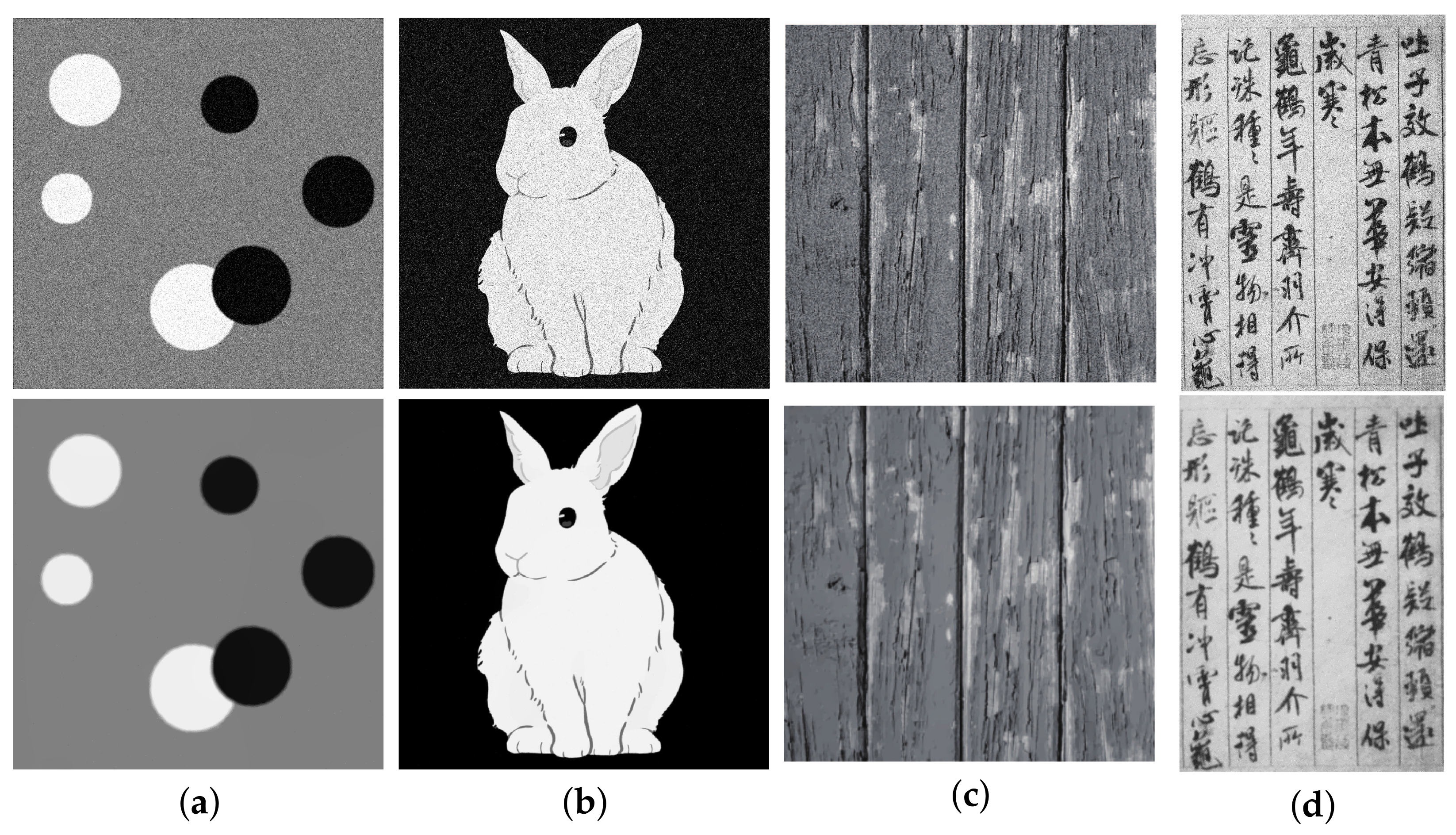
In this subsection, we use four kinds of images, i.e., electronic composite image, JEPG compressed image, photo taken by camera, and scanning image, to demonstrate the effect of our method on the images with 10% Gaussian noise as shown in Figure 1. The top row is the initial images with Gaussian noise and the bottom row is the smoothing results obtained by our method. From Figure 1a–d, the computational domains are with the $256\times 256$, $512\times 512$, $260\times 250$, and $200\times 300$ pixels, respectively. The Non-default parameters are chosen as $\alpha =0.02$, $\beta =0.1$, and $\gamma =0.04$, respectively. It is obvious that the gaussian noise can be eliminate well by the proposed method. Furthermore, some notations should be pointed that: (i) The proposed method can keep a sharp edge while reducing the noise, which can be seen in Figure 1a. (ii) The textures can be smoothed out due to the influence of the soft thresholds, which can be seen in Figure 1b. (iii) The defects in the photos, such as shadows and light spots, are considered as the part of the composition and will not be handled by our algorithm, which can be seen in Figure 1c. (iv) The small non–noisy pixels in the images can be removed due to the influence of the hard thresholds, which can be seen in Figure 1d.

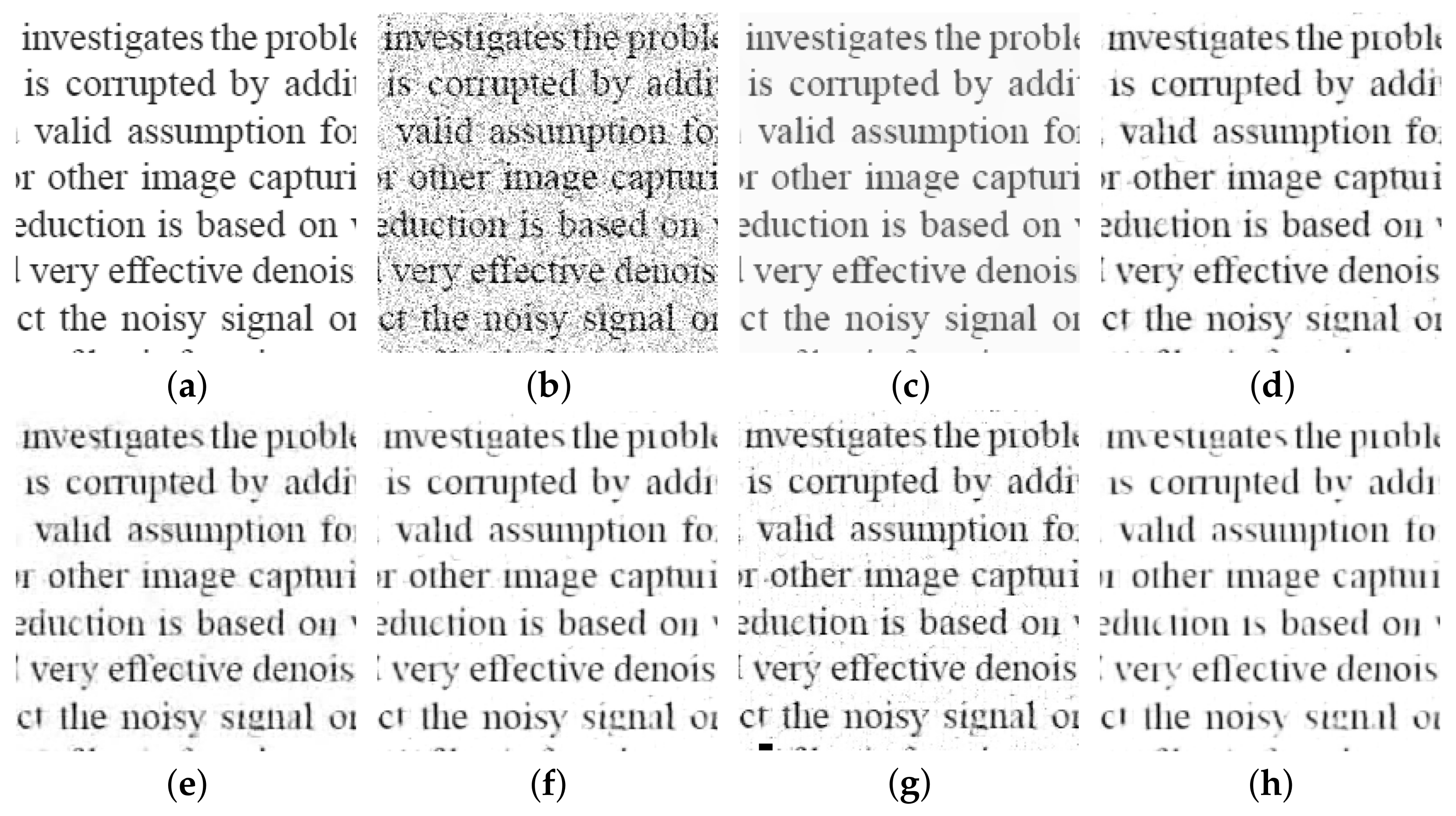
4.2. Noise Reduction for Speckle Noise Processing

Speckle noise is the noise that arises due to the effect of environmental conditions on the imaging sensor during image acquisition, it is common in active radar, synthetic aperture radar, medical ultrasound and optical coherence, and reduces the quality of tomography images [33]. In this subsection, we use the text image, photo taken by camera, remote sensing image, scanning image, to demonstrate the effect of our method on the images with speckle noise as shown in Figure 2. The top row is the initial images with speckle noise and the bottom row is the smoothing results obtained by our method. The computational meshgrid is $100\times 100$, $400\times 400$, $1024\times 1024$, and $120\times 120$, respectively. The non-default parameters are chosen as $\alpha =0.1$, $\beta =0.01$, and $\gamma =0.2$, respectively. It is obvious that the speckle noise can be removed by our method without destroying any features of the noisy images such as edges and the structure. We should emphasize that the speckle noise influence the quality of ultrasound image and it can reduces important information from image as edge, shape, and intensity value, which is easy to handle with our method. Since our method is essentially a weighted average combination of soft threshold and hard threshold, the image edge and shape can be captured well by choosing the proper weight parameters.

4.3. Noise Reduction for Poisson Noise Processing

Poisson noise is a noise model conforming to Poisson distribution, which is suitable to describe the probability distribution of the number of random events in unit time [34]. In this subsection, we use a cartoon image to demonstrate the effect of our method on the images with Poisson noise as shown in Figure 3. From Figure 3a–d, we show the original images with poission noise, the smoothing images by the proposed method, the contour line of (a), and the contour line of (b), respectively. The computational meshgrid is $320\times 320$. We chose the non–default parameters as $\alpha =0.1$, $\beta =0.1$, $\gamma =0.2$, $\zeta =10$, and $\lambda =1000$, respectively. By comparing Figure 1a,b, it can be seen that our algorithm can eliminate gaussian noise without affecting the edges and the shape of the noisy image. To better demonstrate this property, we plot the contour line of the image, which verifies that the proposed method is efficient for obtaining the clean gradient map and in accordiance with human perception.

4.4. Comparison between the Existing Method and the Proposed Method

In this subsection, we compare the results obtained by the proposed method and the existing method, i.e., TID [5], BM3D [6], BM3D-PCA [7], LPG-PCA [8], and NLM [35], to verify the efficiency of the proposed method. We have re-implemented and modified the internal method so that the above methods can be fairly compared with the proposed method. The computational meshgrid is $110\times 110$ and we choose the non–default parameters as $\alpha =0.02$, $\zeta =100$, and $\gamma =0.04$, respectively.

To prepare the numerical test, we added randomly excessive noise to the original image Figure 4a and obtain the test noisy image Figure 4b. We not only perform the corresponding qualitative numerical experiment as shown in Figure 4, but also implies the corresponding quantitative numerical experiment as shown in

Table 1. Comparison of the average PSNR and SSIM between the proposed method and other existing methods.

Methods	Ours	TID	BM3D	BM3DPCA	LPG–PCA	NLM
PSNR	$\mathbf{23.13}$	$22.91$	$21.57$	$21.59$	$22.01$	$20.14$
SSIM	$\mathbf{0.9542}$	$0.8890$	$0.8507$	$0.8551$	$0.7030$	$0.8278$

. It is obvious that our method provide the cleaner results with the same input image in Figure 4. Furthermore, the proposed method globally sharpen prominent edges and remains the text pixel while eliminating the noise. Two metrics, namely peak signal–to–noise ratio (PSNR) and structural similarity index map (SSIM), are quantitative measure used to estimate the quality of the denoised images, which can be defined as

$$\begin{array}{c}\hfill \mathrm{PSNR}=10{log}_{10}\frac{I_{max}^2}{\frac{1}{n_x·n_y}{\sum }_{i=1}^{n_x}{\sum }_{j=1}^{n_y}{\left(I_{i,j}-K_{i,j}\right)}^2}, \mathrm{SSIM}=\frac{(2{\mu }_I{\mu }_K+c_1)(2{\sigma }_{IK}+c_2)}{({\mu }_I^2+{\mu }_K^2+c_1)({\sigma }_I^2+{\sigma }_K^2+c_2)},\end{array}$$

where I is the clean image, K is the denoised image, ${\mu }_I,{\mu }_K$ are the average of I and K, respectively; and ${\sigma }_I^2,{\sigma }_K^2$ are the variance of I and K, respectively. Here, ${\sigma }_{IK}$ is the covariance of I and K, $c_1={\left(0.01L\right)}^2,c_2={\left(0.03L\right)}^2$ with $L=1$. High PSNR and SSIM values indicate a good restore of the fingerprint image [36]. By comparing these two indicators as shown in Table 1, our method shows better utilization of the target image.

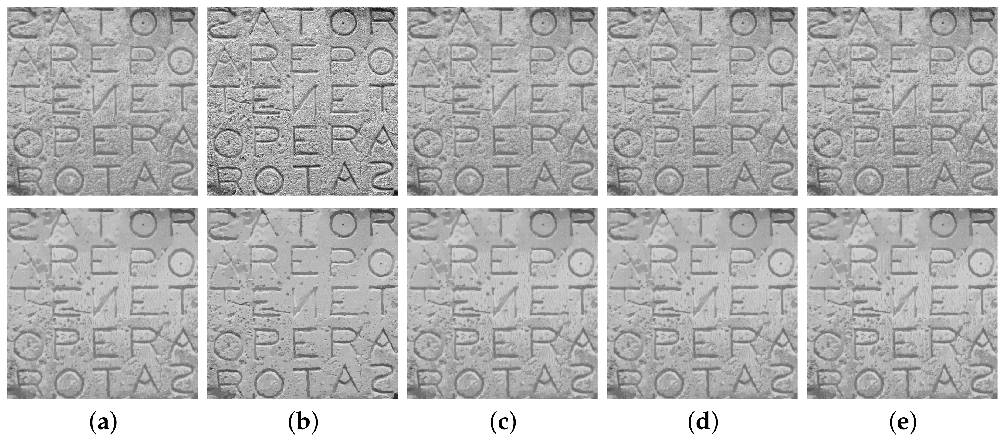
4.5. Comparison between the Smoothing Results with or without Our Method for the Existing Method

In this subsection, we compare the results obtain by the existing method with or without our method. To verify the efficiency of the proposed method, we perform the numerical test on a real scanning image for ancient ruins as shown in Figure 5, which is covered with a dense collection of weathered holes and cracks.

The computational meshgrid is $1000\times 1000$ and the non–default parameters are $\alpha =0.001$, $\gamma =0.002$, and $\zeta =10$, respectively. The smoothing results have been shown in Figure 6.

The top and bottom row shows the results obtained by the existing method without and with our method, respectively. It is obvious that the results obtained with the addition of our method will be smoother. Moreover, we compute the PSNR and SSIM indicators with Equation (21) as shown in

Table 2. Comparison of the average PSNR and SSIM with or without our method for the existing methods.

	TID	BM3D	BM3DPCA	LPG–PCA	NLM
PSNR	$19.03$	$\mathbf{28.64}$	$19.22$	$19.40$	$18.76$
SSIM	$0.5098$	$\mathbf{0.7827}$	$0.5240$	$0.5475$	$0.4849$
Our method+	TID	BM3D	BM3DPCA	LPG–PCA	NLM
PSNR	$26.80$	$\mathbf{31.52}$	$26.66$	$26.90$	$25.81$
SSIM	$0.7208$	$\mathbf{0.9491}$	$0.7230$	$0.7249$	$0.6691$

. For the five existing methods, the combination with our method can significantly improve image quality, which corresponds to our expectation.

4.6. Comparison Test between the Smoothing Results with Deep Learning Image Denoising Schemes and Our Proposed Method

In this subsection, we compare the results obtained by the deep learning image denoising schemes and our proposed method. The existing method denoises the damage images using a MATLAB solver denoisingImage in Deep Learning Toolbox based on the denoising convolutional neural networks(DcNN) [37]. We perform the numerical test on various images types, which are the scanning image, photo taken by camera, and JPEG compressed image, respectively. From Figure 7a–d, the images are the ground truth, image with 10% Gaussian noise, results obtained by our proposed method, respectively.

The computational meshgrid for the top row, middle row, and bottom row is $600\times 500$, $1000\times 500$, and $800\times 700$, respectively. The non–default parameters are $\alpha =0.001$, $\gamma =0.02$, and $\zeta =12$, respectively. As can be seen from the comparable results, our method maintains the similarity with the original image and actively reduces the amplitude gradient difference between the noise points and the surrounding pixels to obtain better results. What we need to emphasize is that our method adaptively adjusts for specific images, which can better process different noise information appropriately. Moreover, the PSNR and SSIM indicators with Equation (21) for Figure 7c,d have been shown in

Table 3. Comparison of the average PSNR and SSIM between the proposed method and DcNN based method in MATLAB.

Ours/DcNN	Top Row	Middle Row	Bottom Row
PSNR	$\mathbf{28.37}$/$24.61$	$\mathbf{24.42}$/$18.47$	$\mathbf{27.68}$/$22.76$
SSIM	$\mathbf{0.9214}$/$0.8463$	$\mathbf{0.7952}$/$0.7264$	$\mathbf{0.9017}$/$0.8911$

. We can see that our method shows better utilization of the target images from the point of perspective view.

We should note that it is unfair for this type comparison in some aspects. The proposed method works well without the training cost, while the DcNN based method require expensive training costs to improve the corresponding accuracy.

4.7. Comparison Test between the Smoothing Results with Existing Structure-Texture Decomposition Method and Our Proposed Method

In this subsection, we compare the results obtained by the existing structure-texture decomposition method and our proposed method. We perform the numerical test on a electronic composite image with complex boundaries and complicated geometry as shown in Figure 8a. Since the boundary is not clear and the covered triangles have different sizes and shapes, it brings hard challenges for boundary extraction. The computational meshgrid is $750\times 1000$ and the non–default parameters are $\alpha =0.0004$, $\gamma =0.002$, and $\zeta =15$, respectively. We add the $10\%$ Gaussian noise to the ground truth (Figure 8a) and obtain the damage image Figure 8b. Figure 8c,d are the denoising results obtain by the method in [38] and our proposed method, respectively. The images in bottom row (Figure 8e,f) show the edge detection results correspond to Figure 8c,d, respectively. As can be seen from the comparable results, the structure-texture method in [38] recognized the edges as the texture of the target images by making the boundary too smooth, while our method can increase the contrast between the two sides of the edges and prominent the boundary.

Moreover, we compute the PSNR and SSIM indicators with Equation (21). The PSNR of Figure 8c,d is $18.24$ and $22.36$, respectively. The SSIM of Figure 8c,d is $0.7634$ and $0.9142$, respectively. Based on the quantitative perspective, our method can significantly improve image quality, which corresponds to our expectation. From the comparison of Figure 8e,f, our method is easier to detect the edges with less errors.

4.8. Computational Cost

Finally, we present the performance of all above tests in

Table 4. Total CPU-time of every numerical test in this work.

Figure	Figure 1a	Figure 1b	Figure 1c	Figure 1d	Figure 2a
CPU-time (s)	5.91	18.34	4.74	3.49	1.57
Figure	Figure 2b	Figure 2c	Figure 2d	Figure 3	Figure 4c
CPU-time (s)	17.94	57.24	2.34	4.76	1.73
Figure	Figure 6	Figure 7 (top)	Figure 7 (middle)	Figure 7 (bottom)	Figure 8
CPU-time (s)	43.36	22.41	34.62	24.84	26.74

and Figure 9. The CPU times for each tests above have been presented in Table 4. Then we compute the average CPU time per iteration. Let us fit the curve with the computational domain size based on the MATLAB routine polyfit functional. The numerical tests are performed in MATLAB on a computer with a 3-GHz CPU and 8GB of RAM. It is obvious from Table 4 that the computational cost of the proposed method is low.

As can be seen from Figure 9, the computational cost is linear with respect to the domain size. Various notations should be remarked as follows: (i) The proposed method does not require the extensive training times to sacrifice an acceptable level of accuracy. (ii) The proposed scheme is based on the partial differential equation, which makes our approach independent of the specific dataset and noise type. (iii) The computational complexity of our approach depends on the fast Fourier transform, which is proved to be $O\left(NlogN\right)$ and is easy to implement from the numerical point of view.

5. Conclusions

In this paper, a novel image restoration method was proposed by coupling with $L_0$, $L_1$ and $L_2$ gradient minimization of weight average combination. The resulting algorithm was developed by using half-quadratic splitting method. Through the optimization formulation, the smoothing step has been performed by using a Poisson approach after two edge-preserving steps. The proposed iterative method is efficient and robust due to the linearity and parallelism of our algorithm, which is easy to implement. To the best of our knowledge, the present study is the first attempt to denoise the damaged images using the competitive combination of hard- and soft-thresholding model. Compared with neural networks based method, our method is more universal due to the adaptive consideration on the pixel information of a single image. The proposed numerical scheme can be performed to a discrete cosine transform (DCT) implementation with the optimal complexity $O\left(NlogN\right)$ per iteration. Several numerical tests were demonstrated to confirm that the proposed method is efficient and robust for producing image processing results with good quality.