
A Finite Element Reduced-Dimension Method for Viscoelastic Wave Equation

School of Digitalized Intelligence Engineering, Hunan Sany Polytechnic College, Changsha 410129, China
Mathematics 2022, 10(17), 3066; https://doi.org/10.3390/math10173066
Submission received: 6 August 2022
/
Revised: 20 August 2022
/
Accepted: 22 August 2022
/
Published: 25 August 2022
(This article belongs to the Section Computational and Applied Mathematics)
Abstract
:In this study, we mainly employ a proper orthogonal decomposition (POD) to lower the dimension for the unknown Crank–Nicolson finite element (FE) (CNFE) solution coefficient vectors of the viscoelastic wave (VW) equation so as to build a reduced-dimension recursive CNFE (RDRCNFE) algorithm, adopt matrix analysis to analyze the stability together with errors to the RDRCNFE solutions, and utilize some numerical experimentations to verify the effectiveness of the RDRCNFE algorithm.
Keywords:
proper orthogonal decomposition; viscoelastic wave equation; reduced-dimension recursive Crank–Nicolson finite element algorithm; stability and error estimationMSC:
65M15; 65N12; 65N351. Introduction
Let () be a bounded open region with the boundary . For convenience, we herein study the following viscoelastic wave (VW) equation with constant coefficients.
Problem 1.
Seekthat meets
in which, , , Δ represents the Laplacian, λ and ϵ are two positive reals, T represents the final moment, and , , , and are four sufficiently smooth known functions.
The VW equation is of real physical significance and is available for depicting natural phenomena such as vibration wave diffusion (see [1,2,3,4]). However, when it includes complicated initial boundary values and a source term or the irregular calculated region , it has no analytical solution. Therefore, we have to seek its approximate numerical solutions (see [1,2,3,4]).
The Crank–Nicolson finite element (FE) (CNFE) algorithm in [4] is one of the best numerical methods for finding the numerical solutions of the VW equation since its CNFE solution is unconditionally stable, but it also includes many unknowns. Hence, the object herein is to lower the dimension of unknown solution vectors in the CNFE algorithm so as to mitigate the CPU runtime, as well as the error accumulating in the calculated procedure.
It has been proven from many numerical experimentations (see, e.g., [4,5,6,7,8,9,10,11,12,13,14,15,16,17,18,19,20,21,22,23,24,25,26,27,28]) that the proper orthogonal decomposition (POD) is one of the most valid methods that reduces the unknowns in the numerical methods. Unfortunately, according to our knowledge, at the moment, there is no study in which the dimension of the unknown CNFE solution vectors for the VW equation is reduced by the POD method. Hence, we herein make use of the POD to lower the dimension of unknown CNFE solution vectors for the VW equation so as to establish the reduced-dimension recursive CNFE (RDRCNFE) algorithm. In this case, the RDRCNFE algorithm possesses the same FE subspace and accuracy as the classical CNFE algorithm, but is distinguished from the dimension reduction methods of FE subspaces in existing works [4,5,8,17] because the accuracy in the dimension reduction methods of FE subspaces would be severely affected by POD dimension reduction. Of course, the RDRCNFE algorithm is also distinguished from the reduced dimension methods of unknown solution vectors for the hyperbolic, parabolic, Sobolev, and unsteady Stokes equations in [10,11,27,28], both technically and theoretically, because the VW equation is far more complex than the hyperbolic, parabolic, Sobolev, and unsteady Stokes equations.
The rest of this paper is arranged as follows. The functional form and matrix form of the CNFE algorithm for the VW equation, the existence, as well as the stability, together with the error estimations for the CNFE solutions are given in Section 2. In Section 3, the RDRCNFE algorithm is constructed with the POD basis vectors generated by the first several CNFE solution vectors, and the stability, as well as the errors for the RDRCNFE solutions are analyzed via matrix analysis, resulting in a very simple theoretical analysis. In Section 4, several numerical experimentations are used to confirm the advantage of the RDRCNFE algorithm. The main conclusions are summarized in Section 5.
2. The CNFE Algorithm
For the sake of convenience in the theoretical analysis, we suppose that and in Section 2 and Section 3.
The Sobolev spaces, as well as the norms used herein are traditional (see [29]). If we set , by using Green’s formula for Problem 1, we may derive the following functional formulation.
Problem 2.
For, seekthat satisfies
whererepresents the inner product inand.
Assume that is a quasi-uniform triangulation onto (see [4]) and the M-dimensional FE subspace is spanned with the normalized bases with respect to the inner product in , i.e., in which may be obtained by orthonormalizing in [29], Section 1.6.3, and () are lth-degree polynomials, namely
For a given positive integer N, we assume that is the time step, is the CNFE solutions at time moments , and . Then, the CNFE algorithm of the functional-form for Problem 2 can be stated as follows.
Problem 3.
Seekthat satisfies
Herein, represents the Ritz projection (see [4]).
By using the normalized bases , the CNFE solutions to Problem 3 can be denoted by the following vector-form:
where and . Thus, Problem 3 may be rewritten in the following matrix form.
Problem 4.
Seekand () that satisfy
where is Gram’s matrix, is the symmetrical positive definite matrix, , , and and are two given vectors that are formed with function values of and at the lth-degree interpolating nodes , respectively.
Lemma 1.
The Gram matrixin Problem 4 meets the estimate:
where, is the Eulerian norm for vector, and α is a positive constant.
The following theorem gives the result for the existence, as well as the stability, together with the convergence of the CNFE solutions to Problem 3 (i.e., Problem 4).
Theorem 1.
Problem 3 (i.e., Problem 4) has a unique sequence of CNFE solutionsthat meet the following stability:
where α represents a generic positive constant that does not depend on h and, which may be unequal at different occurrences. When the solution ϖ to Problem 2 has sufficient smoothness, the set of CNFE solutionsmeets the following error estimations:
Proof.
Because the coefficient matrix of the unknown vectors in the system of Equation (5) is symmetrical positive definite (herein is the identity matrix), while , , and are given, Problem 4 (i.e., Problem 3) has a unique sequence of CNFE solutions.
Taking the inner product by left multiplying the first equation in (5) with , by Cauchy–Schwarz’s inequality, we obtain
It follows that
Noting that and because of the positive definiteness of , from (10), we obtain
which implies that the CNFE solution coefficient vectors to Problem 4 are unconditionally stable. Thereupon, we obtain
Remark 1.
While the meshes ofneed to be adequately subdivided, Problem 4, namely Problem 3, could have many unknowns, resulting in the round-off errors in the computation being quickly accumulated, and it is difficult to obtain satisfying numerical solutions. Hence, it is very necessary to lower the dimension of unknown vectors in Problem 4 by means of the POD technique.
3. The RDRCNFE Algorithm of the VW Equation
3.1. Generation of POD Bases
We first seek the first L solution vectors with Problem 4 and make a snapshot matrix ; here, . We then calculate the positive eigenvalues rank listed degressively together with the corresponding orthogonalized eigenvectors of . We finally obtain a set of POD basis vectors () from the foremost d vectors in , meeting the following equality (see [4]):
Further, the following estimates hold:
Herein, represent the th-dimension orthonormal vectors, whose only nth component is 1.
Remark 2.
Because of, namely the orderofbeing far smaller than the order M of, but their positive eigenvaluesbeing identical, we may first seek the initial d eigenvalues of together with the associated eigenvectors . Thus, we may readily obtain the initial eigenvectors so as to obtain a set of POD bases (). Especially, the ingenious construction for the above snapshot matrix Λ can bring great convenience in the following theoretical analysis.
3.2. Establishment of RDRCNFE Algorithm
If we assume that , , and , we may obtain the initial L RDRCNFE solutions () from (14). Replacing the vectors in Problem 4 with , we can set up the RDRCNFE algorithm as follows.
Problem 5.
Seekandthat satisfy
where () stand for the initial L solution vectors for Problem 4 and and are the same as those for Problem 4.
Remark 3.
It is obvious that Problem 5 has a unique set of RDRCNFE solutionsbecause of the positive definiteness of the matrix. It is worth noting that Problem 5 at every time node only contains d unknowns, whereas Problem 4 has M unknowns at the same time node, but both have the same FE basis functionsand the same accuracy. Hence, Problem 5 is distinctly superior to Problem 4, which means that Problem 5 could not only immensely decrease the unknowns, but could also vastly save the CPU runtime, lessen the rounded-off error accumulation, and enhance the accuracy of the numerical solutions in the actual calculations (see the numerical tests in Section 4).
3.3. The Stability and Error Estimates for the RDRCNFE Solutions
The RDRCNFE solutions to Problem 5 have the following stability, as well as error estimations.
Theorem 2.
Under the identical conditions of Theorem 1, the set of RDRCNFE solutionsto Problem 5 has the unconditional stability together with the following error estimations:
where therepresent the states of the solutionto Problem 1 when.
Proof.
(i) Prove the unconditional stability for the RDRCNFE solutions.
When , using the orthonormality for the POD basis vectors and the unconditional stability of in Theorem 1, we obtain
which signifies that is unconditionally stable.
When , using , we could revert (16) as
Taking the inner product by left multiplying Equation (19) with and using the Cauchy-Schwarz inequality, we gain
It follows that
Owing to the positive definiteness of the matrix , it holds that . Thus, using , as well as , by (11) and (22) we obtain
It follows that
which implies that the RDRCNFE solution vectors for Problem 5 are unconditionally stable. Furthermore, we obtain
(ii) Discuss the error estimations of the RDRCNFE solutions.
When , using and , by (14), we obtain
Taking the inner product by left multiplying Equation (27) with , we obtain
Owing to the positive definiteness of the matrix , it holds that . Thus, using and , by (11) and (29) we obtain
Thereupon, we obtain
Remark 4.
Even though the errors in Theorem 2 have one more error termthan those in Theorem 1, which is brought by adopting the POD technique to reduce the order of Problem 4, it may serve as a criterion to choose the number d of POD bases. Moreover, as long as the selected initial d POD bases meet, it would not make a big difference in the total errors. Especially, Problem 5 includes the same basis functions as Problem 4 so that its accuracy remains the same as Problem 4 in actual applied computations. It has been verified by many numerical simulating tests (see, e.g., [4,5,6,7,8,9,10,11,12,13,27,28]) that the eigenvaluecould rapidly drop off to 0; generally, when or 6, is already very small and satisfies . In particular, if the RDRCNFE solution obtained by Problem 5 at the time node cannot satisfy the desired accuracy, but at the time node still satisfies the accuracy requirement, then we can take a new snapshot matrices (where ) to construct a new set of POD basis vectors so as to construct the new RDRCNFE algorithm to seek the RDRCNFE solutions satisfying the accuracy requirement. Likewise, we can gain the RDRCNFE solutions satisfying the accuracy requirement at an arbitrary time node. This is something that the classical CNFE algorithm cannot do.
4. Some Numerical Experiments
In order to verify the correctness of the theory results and to exhibit the importance of the RDRCNFE algorithm, we herein provide some numerical experiments to show that the VW equation has the analytical solution. Generally, when its initial boundary values and source term are complicated or the calculating region is irregular, there is not an analytical solution.
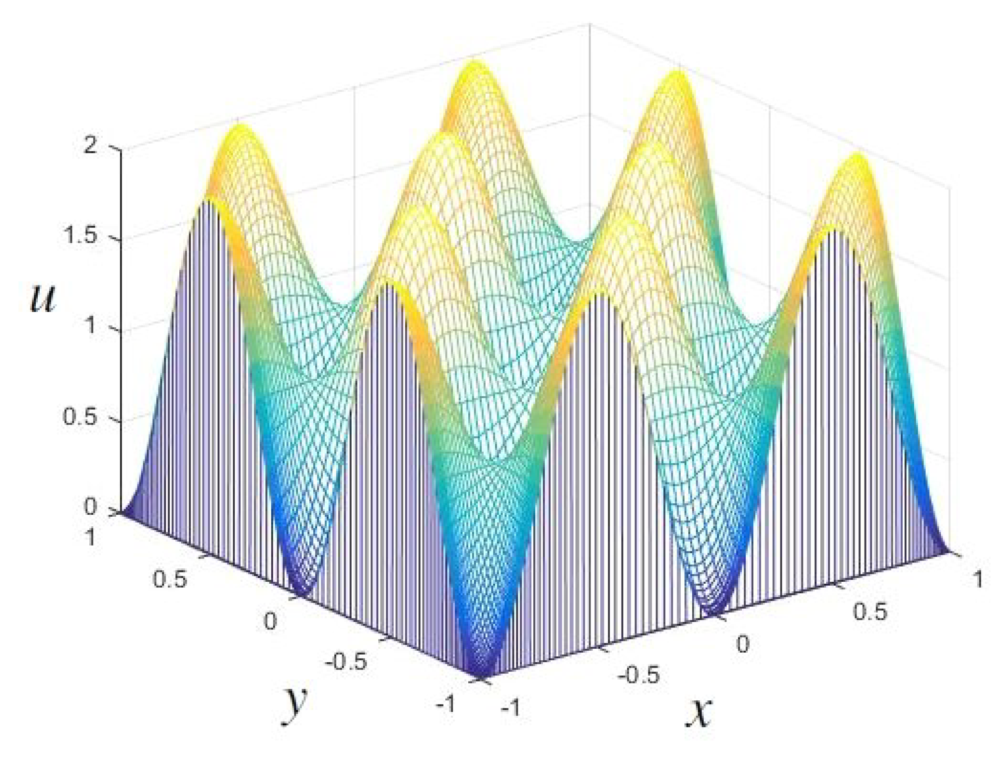
In the VW equation (i.e., Problem 1), we take , , , , (see Figure 1), and . The VW Equation (1) has an analytical solution:
The triangulation on is made up of the isosceles right triangles with the right side parallel to the x and y axes such that . If in Problem 4 consists of the piecewise linear polynomials (i.e., ), , and (here, the constant ), then the theoretical errors of both the CNFE and RDRCNFE solutions are no more than according to Theorems 1 and 2.
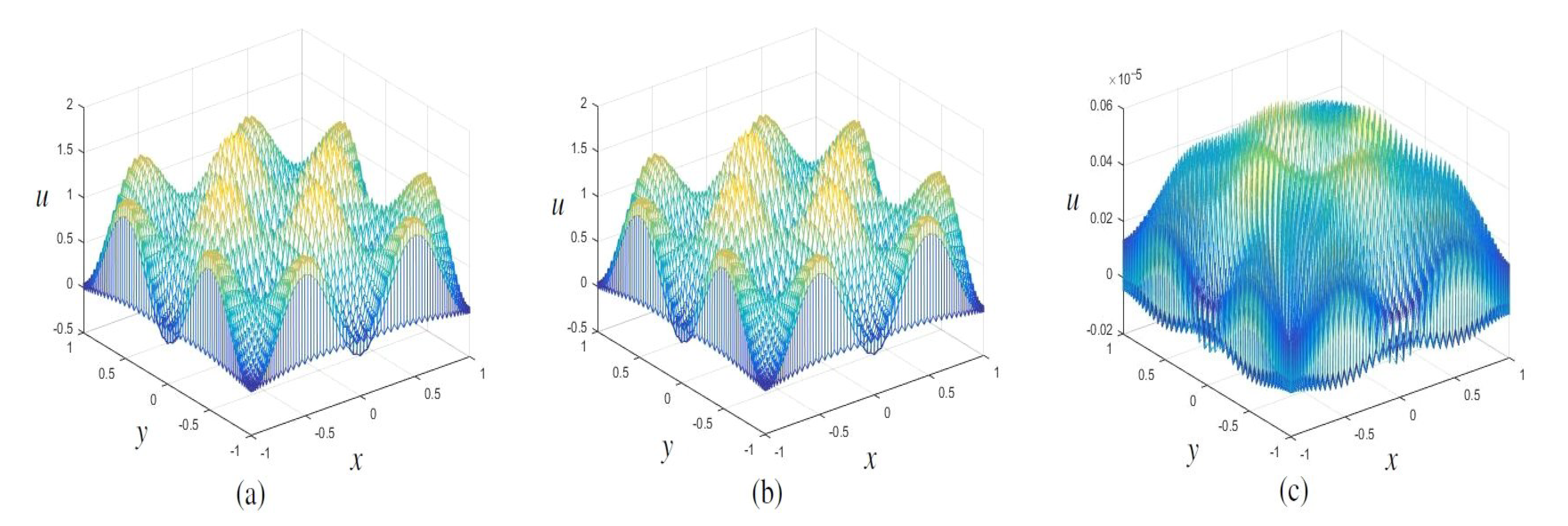
We first find the initial 20 CNFE solutions by Problem 4 and compose the matrix , in which . Afterwards, we compute the eigenvalues for (arranged degressively), so as to estimate that . Hence, we just have to take the initial five eigenvectors of to construct the POD bases with . In the end, the RDRCNFE solutions are solved by Problem 5, exhibited in Figure 2a, Figure 3a and Figure 4a, and the CPU runtime together with the numerical errors between the analytical solutions and RDRCNFE solutions are recorded and listed in Table 1, when , 1000, and 1500 (i.e., , , and ), respectively.
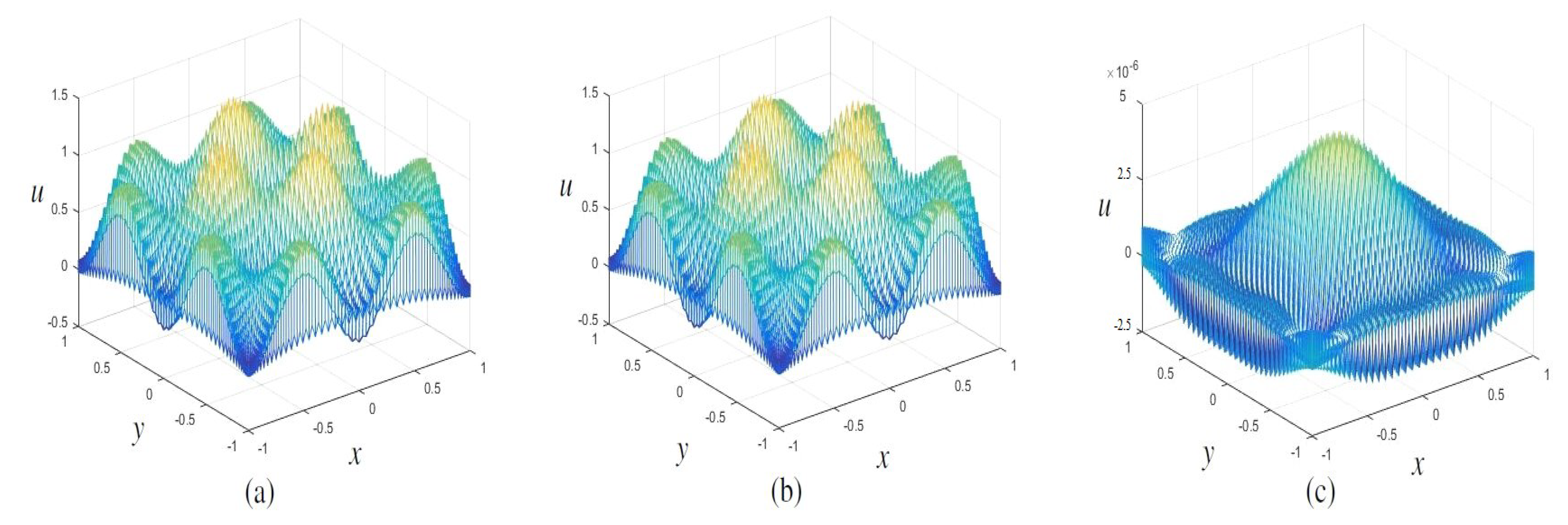
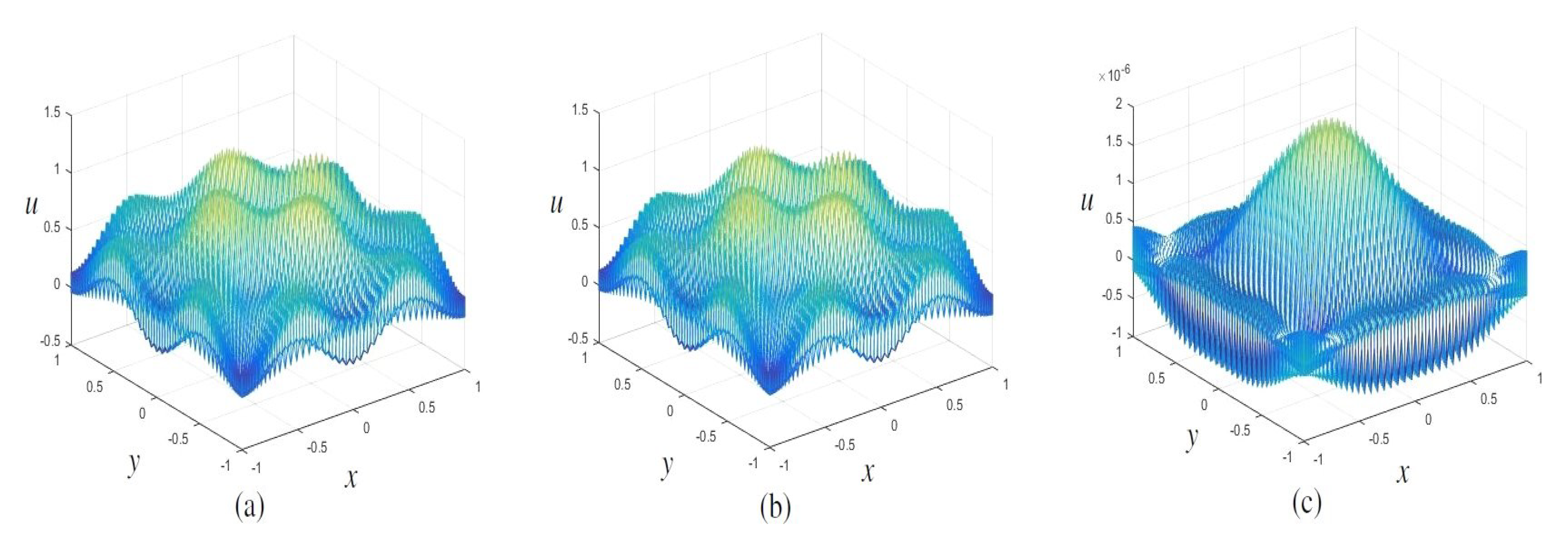
In order to exhibit the importance of the RDRCNFE algorithm, the CNFE solutions are also solved by Problem 4, shown in Figure 2b, Figure 3b and Figure 4b, and the CPU runtime together with the numerical errors between the analytical solutions and the CNFE solution are also recorded and are listed in Table 1, when , 1000, and 1500 (i.e., , , and ), respectively. Moreover, the errors between the CNFE solutions and the RDRCNFE solutions while , , and are, respectively, exhibited in Figure 2c, Figure 3c and Figure 4c, which show that the numerical errors are consistent with the theoretical errors and that the diagrams for the RDRCNFE solutions are almost identical to those for the CNFE solutions.
It follows from Table 1 that the CPU runtime of the RDRCNFE algorithm is far less than that of the classical CNFE algorithm because the RDRCNFE algorithm has only five unknowns at each time node, but the classical CNFE algorithm possesses unknowns at the same time node. Thus, the RDRCNFE algorithm could not only slow down the rounded off error accumulation and mitigate the computational load, but also save the CPU runtime and memory space in the calculation process, as well as improve the calculation efficiency. For example, the CPU runtime of the CNFE algorithm is about 63-times more than that of the RDRCNFE algorithm as . It is indicated that the RDRCNFE algorithm is far better than the CNFE algorithm. Furthermore, it is shown that the RDRCNFE algorithm is effective at settling the VW equation.
5. Conclusions
Herein, we discussed the dimension reduction by the CNFE algorithm for the VW equation. We skillfully made use of the POD to build the RDRCNFE algorithm of the VW equation, adopted the matrix approaches to analyze the stability together with the errors of the RDRCNFE solutions in detail, and accurately used some numerical experimentations to confirm the importance of the RDRCNFE algorithm. The dimension for the RDRCNFE algorithm is far lower than that for the CNFE algorithm, so that it could not only vastly lessen the accumulation of the round-off errors together with the calculation burden, but also vastly save the CPU runtime. In particular, the dimension reduction with respect to the unknown CNFE solution coefficient vectors of the VW equation was developed by the first time, so that the RDRCNFE algorithm is a new contribution and is distinguished from all previous reduced-order methods.
Although, herein, we only studied the RDRCNFE algorithm for the VW equation, the approach can be generalized to more complex real-world engineering problems, as well. Hence, the RDRCNFE algorithm has very comprehensive applications. Moreover, herein, we only considered the following VW equation with constant coefficients. However, when one studies the properties of viscoelastic materials, if one adopts the Prony series representations, one would obtain the more accurate representations of viscoelastic materials (see [30]).
Author Contributions
The author contributed independently and significantly in writing this article. Z.L. independently wrote, read, and approved the final manuscript. All authors have read and agreed to the published version of the manuscript.
Funding
This research was supported by the National Natural Science Foundation of China (11671106) and Qian Science Cooperation Platform Talent ([2017]5726-41).
Institutional Review Board Statement
Not applicable.
Informed Consent Statement
Not applicable.
Data Availability Statement
Not applicable.
Acknowledgments
The author of this paper thanks the anonymous Reviewers and Editors very much for their valuable suggestions.
Conflicts of Interest
The author declares no conflict of interest.
References
- de Saint-Venant, A.J.C. Théorie du mouvement non permanent des eaux, avec application auxcrues des rivers et a l’introduction des marées dans leur lit. Comptes Rendus De L’Académie Des Sci. 1871, 73, 147–154. [Google Scholar]
- Giovangigli, V.; Tran, B. Mathematical analysis of a Saint-Venant model with variable temperature. Math. Mod. Meth. Appl. Sci. 2010, 20, 1251–1297. [Google Scholar] [CrossRef]
- Li, H.; Zhao, Z.H.; Luo, Z.D. A space-time continuous finite element method for 2D viscoelastic wave equation. Bound. Value Probl. 2016, 2016, 53. [Google Scholar] [CrossRef]
- Luo, Z.D.; Chen, G. Proper Orthogonal Decomposition Methods for Partial Differential Equations; Academic Press of Elsevier: San Diego, CA, USA, 2018. [Google Scholar]
- Alekseev, A.K.; Bistrian, D.A.; Bondarev, A.E.; Navon, I.M. On linear and nonlinear aspects of dynamic mode decomposition. Int. J. Numer. Meth. Fluids 2016, 82, 348–371. [Google Scholar] [CrossRef]
- Deng, Q.X.; Luo, Z.D. A reduced-order extrapolated finite difference iterative scheme for uniform transmission line equation. Appl. Numer. Math. 2022, 172, 514–524. [Google Scholar] [CrossRef]
- Du, J.; Navon, I.M.; Zhu, J.; Fang, F.; Alekseev, A.K. Reduced order modeling based on POD of a parabolized Navier-Stokes equations model II Trust region POD 4D VAR data assimilation. Comput. Math. Appl. 2013, 65, 380–394. [Google Scholar] [CrossRef]
- Li, H.R.; Song, Z.Y. A reduced-order energy-stability-preserving finite difference iterative scheme based on POD for the Allen-Cahn equation. J. Math. Anal. Appl. 2020, 491, 124245. [Google Scholar] [CrossRef]
- Li, H.R.; Song, Z.Y. A reduced-order finite element method based on proper orthogonal decomposition for the Allen-Cahn model. J. Math. Anal. Appl. 2021, 500, 125103. [Google Scholar] [CrossRef]
- Luo, Z.D. The reduced-order extrapolating method about the Crank–Nicolson finite element solution coefficient vectors for parabolic type equation. Mathematics 2020, 8, 1261. [Google Scholar] [CrossRef]
- Luo, Z.D.; Jiang, W.R. A reduced-order extrapolated technique about the unknown coefficient vectors of solutions in the finite element method for hyperbolic type equation. Appl. Numer. Math. 2020, 158, 123–133. [Google Scholar] [CrossRef]
- Chaturantabut, S.; Sorensen, D.C. A state space error estimate for POD-DEIM nonlinear model reduction. SIAM J. Numer. Anal. 2012, 50, 46–63. [Google Scholar] [CrossRef]
- Sirovich, L. Turbulence and the dynamics of coherent structures part I–III. Quart. Appl. Math. 1987, 45, 561–590. [Google Scholar] [CrossRef]
- Song, Z.Y.; Li, H.R. Numerical simulation of the temperature field of the stadium building foundation in frozen areas based on the finite element method and proper orthogonal decomposition technique. Math. Method Appl. Sci. 2021, 44, 8528–8542. [Google Scholar] [CrossRef]
- Zhu, S.; Dede, L.; Quarteroni, A. Isogeometric analysis and proper orthogonal decomposition for parabolic problems. Numer. Math. 2017, 135, 333–370. [Google Scholar] [CrossRef]
- Kunisch, K.; Volkwein, S. Galerkin proper orthogonal decomposition methods for a general equation in fluid dynamischs. SIAM J. Numer. Anal. 2002, 40, 492–515. [Google Scholar] [CrossRef]
- Li, K.; Huang, T.Z.; Li, L.; Lanteri, S.; Xu, L.; Li, B. A Reduced-Order Discontinuous Galerkin Method Based on POD for Electromagnetic Simulation. IEEE Trans. Antennas Propag. 2018, 66, 242–254. [Google Scholar] [CrossRef]
- Luo, Z.D.; Wang, H. A highly efficient reduced-order extrapolated finite difference algorithm for time-space tempered fractional diffusion-wave equation. Appl. Math. Lett. 2020, 102, 106090. [Google Scholar] [CrossRef]
- Hinze, M.; Kunkel, M. Residual based sampling in POD model order reduction of drift-diffusion equations in parametrized electrical networks. J. Appl. Math. Mech. 2012, 92, 91–104. [Google Scholar] [CrossRef]
- Stefanescu, R.; Navon, I.M. POD/DEIM nonlinear model order reduction of an ADI implicit shallow water equations model. J. Comput. Phys. 2013, 237, 95–114. [Google Scholar] [CrossRef]
- Zokagoa, J.M.; Soulaïmani, A. A POD-based reduced-order model for free surface shallow water flows over real bathymetries for Monte-Carlo-type applications. Comput Methods Appl. Mech. Eng. 2012, 221–222, 1–23. [Google Scholar] [CrossRef]
- Baiges, J.; Codina, R.; Idelsohn, S. Explicit reduced-order models for the stabilized finite element approximation of the incompressible Navier-Stokes equations. Int. J. Numer. Methods Fluids 2013, 72, 1219–1243. [Google Scholar] [CrossRef]
- Luo, Z.D.; Jin, S.J. A reduced-order extrapolated Crank–Nicolson collocation spectral method based on POD for the 2D viscoelastic wave equations. Numer. Meth. Partial Differ. Equ. 2020, 36, 49–65. [Google Scholar] [CrossRef]
- Benner, P.; Cohen, A.; Ohlberger, M.; Willcox, A.K. Model Rduction and Approximation Theory and Algorithm; Computational Science & Engineering; SIAM: Philadelphia, PA, USA, 2017. [Google Scholar]
- Quarteroni, A.; Manzoni, A.; Negri, F. Reduced Basis Methods for Partial Differential Equations; Springer International Publishing: Manila, Philippines, 2016. [Google Scholar]
- Yang, J.; Luo, Z.D. Proper orthogonal decomposition reduced-order extrapolation continuous space-time finite element method for the two-dimensional unsteady Stokes equation. J. Math. Anal. Appl. 2019, 475, 123–138. [Google Scholar] [CrossRef]
- Zeng, Y.H.; Luo, Z.D. The reduced-dimension technique for the unknown solution coefficient vectors in the Crank–Nicolson finite element method for the Sobolev equation. J. Math. Anal. Appl. 2022, 513, 126207. [Google Scholar] [CrossRef]
- Luo, Z.D. The dimensionality reduction of Crank–Nicolson mixed finite element solution coefficient vectors for the unsteady Stokes equation. Mathematics 2022, 10, 2273. [Google Scholar] [CrossRef]
- Zhang, G.; Lin, Y. Notes on Functional Analysis; Peking University Press: Beijing, China, 1987. (In Chinese) [Google Scholar]
- Ghoreishy, M.H.R. Determination of the parameters of the Prony series in hyper-viscoelastic material models using the finite element method. Mater. Des. 2012, 35, 791–797. [Google Scholar] [CrossRef]
Figure 1.
The initial function .

Figure 2.
(a) The RDRCNFE solution when . (b) The CNFE solution when . (c) The error between the RDRCNFE solution and the CNFE solution when .
Figure 2.
(a) The RDRCNFE solution when . (b) The CNFE solution when . (c) The error between the RDRCNFE solution and the CNFE solution when .

Figure 3.
(a) The RDRCNFE solution when . (b) The CNFE solution when . (c) The error between the RDRCNFE solution and the CNFE solution when .
Figure 3.
(a) The RDRCNFE solution when . (b) The CNFE solution when . (c) The error between the RDRCNFE solution and the CNFE solution when .

Figure 4.
(a) The RDRCNFE solution when . (b) The CNCS solution when . (c) The error between the RDRCNFE solution and the CNFE solution when .
Figure 4.
(a) The RDRCNFE solution when . (b) The CNCS solution when . (c) The error between the RDRCNFE solution and the CNFE solution when .


Table 1.
The errors between the analytical solution and the CNFE with RDRCNFE solutions and the CPU runtime.
Table 1.
The errors between the analytical solution and the CNFE with RDRCNFE solutions and the CPU runtime.
| t | n | CPU Runtime | CPU Runtime | ||
|---|---|---|---|---|---|
| 500 | 2.224293 | 88.897 s | 2.361843 | 2.478 s | |
| 1000 | 4.227492 | 187.957 s | 4.963873 | 3.692 s | |
| 1500 | 6.746293 | 273.375 s | 5.663234 | 4.323 s |
Publisher’s Note: MDPI stays neutral with regard to jurisdictional claims in published maps and institutional affiliations. |
© 2022 by the author. Licensee MDPI, Basel, Switzerland. This article is an open access article distributed under the terms and conditions of the Creative Commons Attribution (CC BY) license (https://creativecommons.org/licenses/by/4.0/).
Share and Cite
MDPI and ACS Style
Luo, Z. A Finite Element Reduced-Dimension Method for Viscoelastic Wave Equation. Mathematics 2022, 10, 3066. https://doi.org/10.3390/math10173066
AMA Style
Luo Z. A Finite Element Reduced-Dimension Method for Viscoelastic Wave Equation. Mathematics. 2022; 10(17):3066. https://doi.org/10.3390/math10173066
Chicago/Turabian StyleLuo, Zhendong. 2022. "A Finite Element Reduced-Dimension Method for Viscoelastic Wave Equation" Mathematics 10, no. 17: 3066. https://doi.org/10.3390/math10173066
Note that from the first issue of 2016, this journal uses article numbers instead of page numbers. See further details here.