Review of Methods, Applications and Publications on the Approximation of Piecewise Linear and Generalized Functions

Abstract

Approximation of piecewise linear and generalized functions is an important and difficult problem. These functions are widely used in mathematical modeling of various processes and systems, such as: automatic control theory, electrical engineering, radio engineering, information theory and transmission of signals and images, equations of mathematical physics, oscillation theory, differential equations and many others. The widespread use of such functions is explained by their positive properties. For example, piecewise linear functions are characterized by a simple structure over segments. However, these features also have disadvantages. For example, in the case of using piecewise linear functions, solutions have to be built in segments. In this case, the problem of matching the obtained solutions at the boundaries of the segments arises, which leads to the complication of the research results. The use of generic functions has similar disadvantages. To eliminate shortcomings in practice, one resorts to the approximation of these functions. There are a large number of well-known methods for approximating piecewise linear and generalized functions. Recently, new methods for their approximation have been developed. In this study, an attempt was made to generalize and discuss the existing methods for approximating the considered functions. Particular emphasis is placed on the description of new approximation methods and their applications in various fields of science and technology. The publication-based review discusses the strengths and weaknesses of each method, compares them, and considers suitable application examples. The review will undoubtedly be interesting not only for mathematicians, but also for specialists and scientists working in various applied fields of research.

1. Introduction

In many areas of mathematics and its applications, a problem often arises related to replacing functions that are complex or inconvenient in one sense or other with simpler ones, but close to the original ones. This problem is called the approximation of functions. In many areas of mathematics and its applications, the problem often arises of replacing functions that are complex or inconvenient in one sense or other with simpler ones, but close to the original ones. A number of studies have been devoted to solving this problem, and a large amount of scientific and educational literature has been published. As an example, one can point to the fundamental books [1,2,3,4] and many others.

The review considers methods of approximation of piecewise linear and generalized functions [5,6,7,8,9,10,11,12,13,14,15,16,17], which are universal and find wide application for solving a variety of problems related to mathematical modeling of systems, processes and phenomena described using such functions.

Piecewise linear and generalized functions are widely used in various fields of scientific research. Their traditional fields of application are technical and mathematical disciplines, for example, automatic control theory, electrical engineering, radio engineering, information theory and transmission of signals and images, equations of mathematical physics, oscillation theory, differential equations and many others [18,19,20,21,22,23,24]. Using such functions, for example, they describe the dynamics of mechanical systems with nonlinear elasticities, elastic-dissipative characteristics of vehicle suspensions, systems with loads of the “dry friction” type, impulse transformations during transmission and reception of signals, distributed and concentrated loads, and many other processes.

The widespread use of piecewise linear functions is explained by the simplicity of their structure, especially by areas. At each site, these functions are straight lines and their segments, which in many cases allows one to obtain solutions using the methods of the theory of linear systems. At the same time, problems often arise when constructing solutions over the entire domain of definition of piecewise-linear functions, linking solutions for sections with the need to use special mathematical methods. Systems with piecewise linear characteristics and functions are referred to as essentially nonlinear structures, emphasizing the complexity of obtaining solutions for such structures. Despite the simplicity of piecewise linear functions over sections, the construction of solutions in problems with piecewise linear functions over the entire domain of definition requires the use of special mathematical methods, for example, the matching method [25], with the need to match solutions over sections and switching surfaces. So, when constructing periodic solutions, it is necessary to monitor the fulfillment of the conditions for the transition of the system from section to section, fixing the values of the variables at the end of the previous section and taking these values as the initial conditions for the next section. The need to match the values of the variables over the sections, as well as at the beginning and end of the cycle, leads to a cumbersome system of transcendental equations. Therefore, the application of the fitting method often requires overcoming significant mathematical difficulties, and even if the periodic solution can be found in analytical form, it is usually obtained in the form of complex expressions. In addition, the derivatives of piecewise linear functions are not continuous, which in some cases also complicates research. To simplify calculations, one often resorts to approximating piecewise linear functions. The existing approximation methods have their drawbacks.

Generalized functions were introduced in connection with the problems of physics and mathematics that appeared in the twentieth century and required a new understanding of the concept of a function. Such problems include the problems of determining the density of a point mass, the intensity of a point charge and a point dipole, problems of quantum theory and many others. Generalized functions are now widely used in a wide variety of research areas. For example, generalized functions and their derivatives represent a very convenient mathematical tool for developing control systems. The use of impulse controls significantly increases the control capabilities of various systems. An example of a generalized function is the δ-function or the Dirac function.

Generalized singular functions are very different from regular functions. In many practical applications, these unusual functions are used as purely abstract mathematical constructions, completely divorced from their physical understanding. This approach does not seem to be correct. For a better understanding of generalized functions and a conscious decision on their basis of practical problems, you can use the approximations of these functions. Some of these possible approximations are suggested in this review.

The content of the new methods is explained by a number of practical examples. The examples given are taken from a wide variety of fields: structural mechanics, medicine, quantum theory, signal theory, semiconductor theory, mechanical engineering, heat engineering, and others. The variety of the considered examples emphasizes the rather broad possibilities of practical application of the conceded approximation methods. Therefore, the review will undoubtedly be interesting not only for mathematicians, but also for specialists and scientists working in various applied fields of research.

2. Basic Provisions and Methods of Approximation Theory

This section of the review introduces the basic concepts of approximation theory, discusses the canonical methods of approximation of continuous and discontinuous functions [26,27,28,29]. The considered methods are illustrated with examples, the positive and negative sides of these methods are noted.

2.1. The Main Idea of the Approximation of the Original Function: Basic Concepts

Let $M$ be some point set in $n$-ddimensional space and let $f\left(A\right), A\in M$ be some function defined on this set. This function $f\left(A\right)$, due to some considerations that we will talk about below, we want to replace with other, the so-called approximation function $\phi \left(A,B_1, B_2, \dots , B_k\right)$, also defined on the set $M$, where $B_1, B_2, \dots , B_k$ are parameters. It is necessary to determine the parameters so that the deviation of the function $\phi \left(A,B_1, B_2, \dots , B_k\right)$ from the original function $f\left(A\right)$ would be the least according to some criteria.

It is clear that the meaning of such a replacement will be only when the original function does not suit us in some way, and therefore we want to go to a function as close to the original, as possible, but devoid of shortcomings of the original function. For example, dissimilar to the original function $f\left(A\right),$ the approximation function $\phi \left(A,B_1, B_2, \dots , B_k\right)$ can have a simpler structure, be continuous, differentiable, analytical, allow the use of any mathematical methods and so on. The approximation function must belong to a certain type of function, which has these advantages over the original function and the properties of functions of this type are well studied in mathematics. For example, an algebraic polynomial, a fractional rational function, a trigonometric sum, a spline function, and so on can act as an approximation function.

When constructing an approximating function, the question arises: what is to be understood by the deviation, or, in other words, by the proximity of functions, to determine the approximation error. To solve this issue, the concepts of metric and metric space are introduced in functional analysis.

Definition 1.

A set $Y$ is called a metric space if each pair of its elements $f_1$ and $f_2$ is associated with a real number $\rho \left(f_1,f_2\right)\ge 0$, for which the following axioms hold:

1.

Identity axiom: $\rho \left(f_1,f_2\right)=0$ if and only if $f_1=f_2$;

2.

Symmetry axiom: $\rho \left(f_1,f_2\right)=\rho \left(f_2,f_1\right)$;

3.

Triangle axiom: $\rho \left(f_1,f_2\right)+\rho \left(f_2,f_3\right)\ge \rho \left(f_1,f_3\right)$, for $\forall f_3\in Y$.

This number $\rho \left(f_1,f_2\right)$ is called the metric of the set $Y$ or the distance between the elements $f_1$ and $f_2$.

Within the framework of this monograph, we mainly consider the issues of approximation of such mathematical objects as functions. In this case, the elements (points) of the sets under consideration are functions. Therefore, we will often denote points of sets and spaces by the letter symbol $f$, as is conducted in the above definition of a metric space.

Consider examples of metrics and metric spaces that are important from the point of view of approximation of functions.

1.

Let $Y$ be the set of all continuous functions on the segment $\left[a,b\right]$. As a metric, we can take the maximum modulus of the difference $\rho \left(f_1,f_2\right)=\underset{x\in \left[a,b\right]}{\max }\left|f_1\left(x\right)-f_2\left(x\right)\right|$.

Without losing the generality of reasoning, the segment $\left[a,b\right]$ with the introduction of a new variable can always be reduced to the segment [0,1]. Therefore, the set of all continuous functions defined on a closed interval with the metric introduced in this way is called the space of all continuous functions and is denoted by $C\left[0,1\right]$;

2.

Let $Y$ be a set of all real bounded functions on the interval [0,1]. In this case, as a metric, we can take the supremum of the modulus of the difference $\rho \left(f_1,f_2\right)=\underset{x\in \left[0,1\right]}{\sup }\left|f_1\left(x\right)-f_2\left(x\right)\right|$.

The set of all real bounded functions with the metric introduced in this way is called the space $M\left[0,1\right]$. It is clear that $C\left[0,1\right]$⊂$M\left[0,1\right]$;

3.

Let $Y$ be the set of all measurable functions defined on the interval [0, 1]. Two functions that differ only on a set of measure zero (coinciding almost everywhere) will be considered identical. As a metric, we can take the equality $\rho \left(f_1,f_2\right)={\displaystyle {\int }_0^1}\frac{\left|f_1\left(x\right)-f_2\left(x\right)\right|}{1+\left|f_1\left(x\right)-f_2\left(x\right)\right|}dx$. Such a space is called the space $S\left[0,1\right]$. Convergence in this space is convergence in measure, that is, a sequence of elements $f_n\to f, \mathrm{if} \rho \left(f_n,f\right)\underset{n\to \infty }{\to } 0$;

4.

Let $Y$ be the set of all functions with integrable $p$-th power on the interval [0,1]. Recall that a function $f\left(x\right)$ is called a function with integrable $p$-th power on the interval $\left[a,b\right]$, if ${\displaystyle {\int }_a^b}{\left|f\left(x\right)\right|}^{p}dx<\infty$. The integral is considered in the sense of Lebesgue. As in the previous case, we will consider two functions that differ only on a set of measure zero to be identical. In this case, as a metric, we can take the integral $\rho \left(f_1,f_2\right)={\left({\displaystyle {\int }_a^b}{\left|f_1\left(x\right)-f_2\left(x\right)\right|}^{p}dx\right)}^{\raisebox{1ex}{$1$}\!\left/ \!\raisebox{-1ex}{$p$}\right.}$. Such a space is called the space $L_p\left[0,1\right]$. For $p=2$ we obtain the so-called functional Hilbert space.

In the further description, we need concepts such as norm and linear normed space.

Definition 2.

A set $E$ is called a linear space if the operations of adding elements and multiplying an element by a number are defined in this set, and for any elements $f_1, f_2, f_3\in E$ and for any numbers $\alpha ,\beta$ the conditions are met:

1.

$f_1+f_2=f_2+f_1$;

2.

$\left(f_1+f_2\right)+f_3=f_1+\left(f_2+f_3\right)$);

3.

$f_1+0=f_1$;

4.

$f_1+\left(-f_1\right)=0$;

5.

$\alpha \left(f_1+f_2\right)=\alpha f_1+\alpha f_2$;

6.

($\alpha +\beta$)$f_1=\alpha f_1+\beta f_2$;

7.

$\alpha \left(\beta f_1\right)=\left(\alpha \beta \right)f_1$;

8.

$1·f_1=f_1$.

Definition 3.

The norm of an arbitrary element $f$ of the set $E$ is a nonnegative number, which is denoted by $\Vert f\Vert$, for which the conditions are met:

1.

$\Vert f\Vert =0\iff f=0$;

2.

$\Vert \alpha ·f\Vert =\left|\alpha \right|·\Vert f\Vert$;

3.

$\Vert f_1+f_2\Vert \le \Vert f_1\Vert +\Vert f_2\Vert$.

Definition 4.

The linear space $E$ with the introduced norm is called a normed linear space.

A metric in a normed linear space can be introduced using the equality $\rho \left(f_1,f_2\right)=\Vert f_1-f_2\Vert$. Convergence in a normed linear space is convergence in the norm, that is, a sequence of elements $f_n\to f, \mathrm{if} \Vert f_n-f\Vert \underset{n\to \infty }{\to } 0$.

Let us give examples of some normed linear spaces that are of great importance from the point of view of approximation theory.

1.

The space of all continuous functions $C\left[0,1\right]$ with operations of addition and multiplication by a number, defined in the usual way. The norm is introduced by the relation $\Vert f\Vert$ = $\underset{x}{\max }\left|f\left(x\right)\right|$;

2.

The space $L_p\left[0,1\right]$ of all functions with integrable $p$-th power on the interval [0,1] with operations of addition and multiplication by a number, defined in the usual way. We introduce a norm in the space of such functions using the equality $\Vert f\Vert ={\left({\displaystyle {\int }_a^b}{\left|f\left(x\right)\right|}^{p}dx\right)}^{\raisebox{1ex}{$1$}\!\left/ \!\raisebox{-1ex}{$p$}\right.}$;

3.

The space of all continuous functions on the segment [0,1] with derivatives continuous on this segment up to the $k$-th order inclusive. The notation for such a space is $C^k$ [0,1]. As a norm in this space, one usually takes the relation $\Vert f\Vert =\max \left\{\underset{x}{\max }\left|f\left(x\right)\right|\right., \underset{x}{\max }\left|f^{\prime }\left(x\right)\right|,\dots$, $\left.\underset{x}{\max }\left|f^{\left(k\right)}\left(x\right)\right|\right\}.$

The basic idea of approximation in a normed linear space can be expressed by the following theorem.

Theorem 1.

Let $E$ be some normed linear space in which the elements $f_1, f_2, \dots ,f_n$ are linearly independent. Let some element $f\in E$ be given. For the element $f$ one can choose such numbers ${\lambda }_1,{\lambda }_2, \dots , {\lambda }_n$, that the value $\Delta \left({\lambda }_1,{\lambda }_2, \dots , {\lambda }_n\right)=\Vert f-\left({\lambda }_1{f}_1+{\lambda }_2{f}_2+\dots +{\lambda }_n{f}_n\right)\Vert$ obtains the smallest value.

Let us present the proof of the theorem [22].

Let ${\lambda }_1^{\ast },{\lambda }_2^{,\ast },\dots , {\lambda }_n^{\ast }$ be an arbitrary set of numbers

Using the reverse triangle inequality, we estimate the modulus of the difference

$$\left|\Delta \left({\lambda }_1^{\ast },{\lambda }_2^{,\ast },\dots , {\lambda }_n^{\ast }\right)-\Delta \left({\lambda }_1,{\lambda }_2, \dots , {\lambda }_n\right)\right|=\left|\Vert f-{\displaystyle \sum }_{k=1}^n{\lambda }_k^{\ast }{f}_k\Vert -\Vert f-{\displaystyle \sum }_{k=1}^n{\lambda }_k{f}_k\Vert \right|\le \Vert {\displaystyle \sum }_{k=1}^n\left({\lambda }_k^{\ast }-{\lambda }_k\right)f_k\Vert \le {\displaystyle \sum }_{k=1}^n\left|{\lambda }_k^{\ast }-{\lambda }_k\right|\Vert f_k\Vert \le \underset{k}{\max }\left|{\lambda }_k^{\ast }-{\lambda }_k\right|·{\displaystyle \sum }_{k=1}^n\Vert f_k\Vert .$$

Therefore, for (${\lambda }_1^{\ast },{\lambda }_2^{,\ast },\dots , {\lambda }_n^{\ast }$) $\underset{}{\to }$ (${\lambda }_1,{\lambda }_2, \dots , {\lambda }_n$) we obtain that $\left({\lambda }_1^{\ast },{\lambda }_2^{,\ast },\dots , {\lambda }_n^{\ast }\right)\underset{}{\to }\Delta \left({\lambda }_1,{\lambda }_2, \dots , {\lambda }_n\right)$. Therefore, the function $\Delta \left({\lambda }_1^{\ast },{\lambda }_2^{,\ast },\dots , {\lambda }_n^{\ast }\right)$ is continuous.

Consider a continuous function Ω $\left({\lambda }_1,{\lambda }_2, \dots , {\lambda }_n\right)=\Vert {\lambda }_1{f}_1+{\lambda }_2{f}_2+\dots +{\lambda }_n{f}_n\Vert$.

The continuity of the function Ω$\left({\lambda }_1,{\lambda }_2, \dots , {\lambda }_n\right)$ can be proved similarly to the proof of the continuity of the function $\Delta \left({\lambda }_1^{\ast },{\lambda }_2^{,\ast },\dots , {\lambda }_n^{\ast }\right)$.

The sphere ${\displaystyle {\sum }_{k=1}^n}{\left|{\lambda }_k\right|}^2$ is a bounded closed set in a finite-dimensional Euclidean space, therefore, based on the well-known Weierstrass theorem, the function Ω $\left({\lambda }_1,{\lambda }_2, \dots , {\lambda }_n\right)$ attains its minimum on this set, which we denote by $m$. Note that $m$> 0, since the function Ω$\left({\lambda }_1,{\lambda }_2, \dots , {\lambda }_n\right)$ is a norm, and the elements $f_1, f_2, \dots ,f_n$ are linearly independent.

Let $\overline{\Omega }$≥ 0 be some lower bound for the set of values of the function Ω$\left({\lambda }_1,{\lambda }_2, \dots , {\lambda }_n\right)$.

If $\sqrt{{\displaystyle {\sum }_{k=1}^n}{\left|{\lambda }_k\right|}^2}>\frac{1}{m}\left(\overline{\Omega }+1+\Vert f\Vert \right)$= R, then, it is easy to obtain

$$\Delta \left({\lambda }_1,{\lambda }_2, \dots , {\lambda }_n\right)\ge \Vert {\lambda }_1{f}_1+{\lambda }_2{f}_2+\dots +{\lambda }_n{f}_n\Vert -\Vert f\Vert \ge \sqrt{{\displaystyle {\sum }_{k=1}^n}{\left|{\lambda }_k\right|}^2}m-\Vert f\Vert >\overline{\Omega }+1,$$

therefore, to find the minimum, we can consider the function $\left({\lambda }_1,{\lambda }_2, \dots , {\lambda }_n\right)$ only in a closed bounded domain ${\sum }_{k=1}^n{\left|{\lambda }_k\right|}^2<R^2$. According to the well−known Weierstrass theorem, a continuous function reaches its minimum in such a domain. Therefore, there are numbers ${\lambda }_1,{\lambda }_2, \dots , {\lambda }_n$, that provide the best approximation of the element $f$ by the linear combination ${\lambda }_1{f}_1+{\lambda }_2{f}_2+\dots +{\lambda }_n{f}_n$.

2.2. Contraction Mapping Principle

The contraction mapping principle is one of the most important mathematical achievements and is widely used to prove existence and uniqueness theorems, find solutions to equations of various types by the method of successive approximations, and prove the convergence of iterative procedures used, for example, in approximation theory. The contraction mapping principle was formulated by the Polish mathematician S. Banach [30,31,32,33,34].

First, we give the following definition.

Let $Y$ be some metric space and $\left\{f_n\right\}$—a sequence of elements of this space.

Definition 5.

A sequence $\left\{f_n\right\}$ is called Cauchy sequence, if for any positive number $\epsilon$ there is a number $N_0$, depending on ε, such that for any numbers $n$ and $m$ it follows from the condition $n, m\ge N_0$ than $\rho \left(f_n,f_m\right)<\epsilon$.

In quantifiers, this definition will be written as follows

$$\forall \epsilon >0 \exists N_0=N_0\left(\epsilon \right)\in N \forall n,m\in N: n,m>N_0\Rightarrow \rho \left(f_n,f_m\right)<\epsilon .$$

A space $Y$ is called complete, if any Cauchy sequence converges to some limit that is an element of the same space.

Theorem 2.

 (Principle of contraction mappings). Let $Y$ be a complete metric space, in which some operator $A$, s given, transforming elements of a given space into elements of the same space, i.e., $A$:$Y\to Y$. Let, for any $f,\phi \in Y$, there exist a number $\alpha <1$, independent of $f$ and $\phi$, such that the condition $\rho \left(Af,A\phi \right)\le \alpha \rho \left(f,\phi \right)$ is satisfied. Then, there is a single element (point) $f_0:A{f}_0=f_0$. This point is called the fixed point of the operator $A$.

 Proof.

Let $f$ be an arbitrary fixed element of the set $Y$.

Let us create a sequence $f_1=Af, f_2=A{f}_1, \dots , f_n=A{f}_{n-1}, \dots$, which is fundamental. Really,

$$\begin{gathered} \rho \left(f_1,f_2\right)=\rho \left(Af,A{f}_1\right)\le \alpha \rho \left(f,Af\right), \\ \rho \left(f_2,f_3\right)=\rho \left(A{f}_1,A{f}_2\right)\le \alpha \rho \left(f_1,f_2\right)\le {\alpha }^2\alpha \rho \left(f,Af\right) \mathrm{and} \mathrm{so} \mathrm{on}. \end{gathered}$$

We obtain, $\rho \left(f_n,f_{n+1}\right)\le {\alpha }^n\alpha \rho \left(f,Af\right)$.

By the triangle axiom for the metric, we write

$$\begin{gathered} \rho \left(f_n,f_{n+p}\right)\le \rho \left(f_n,f_{n+1}\right)+\rho \left(f_{n+1},f_{n+2}\right)+\dots +\rho \left(f_{n+p-1},f_{n+p}\right) \\ \le ({\alpha }^n+{\alpha }^{n+1}+\dots +{\alpha }^{n+p-1}) \rho \left(f,Af\right)=\frac{{\alpha }^n-{\alpha }^{n+p}}{1-\alpha }\rho \left(f,Af\right), p\in N. \end{gathered}$$

Taking into account that α < 1, we obtain $\rho \left(f_n,f_{n+p}\right)\le \frac{{\alpha }^n}{1-\alpha }\rho \left(f,Af\right)$.

Therefore, $\rho \left(f_n,f_{n+p}\right)\underset{n\to \infty }{\to }0$. Therefore, the sequence $\left\{f_n\right\}$ is fundamental, and since, by the hypothesis of the theorem, the space $Y$ is complete, there is an element $f_0\in Y: \underset{n\to \infty }{\lim }{f}_n=f_0$.

Let us show that this element $f_0$ is a fixed point.

Really,

$$\rho \left(f_0,A{f}_0\right)\le \rho \left(f_0,f_n\right)+\rho \left(f_n,A{f}_0\right)=\rho \left(f_0,f_n\right)+\rho \left(A{f}_{n-1},A{f}_0\right)\le \rho \left(f_0,f_n\right)+\alpha \rho \left(f_{n-1},f_0\right).$$

Take an arbitrary number $\epsilon >0$. Since the sequence $\left\{f_n\right\}$ converges to the element $f_0$, then, there is a number $N_1$, for which for any $n\ge N_1$ the condition $\rho \left(f_0,f_n\right)<\frac{\epsilon }{2}$, will be satisfied, and there is a number $N_2$, for which for any $n\ge N_2$ the condition $\alpha \rho \left(f_{n-1},f_0\right)<\frac{\epsilon }{2}$ is satisfied.

Then, we obtain

$$\forall \epsilon >0 \exists N\left(\epsilon \right)=\max {\left\{N_1, N_2\right\}}_{}\forall n: n>N\Rightarrow \rho \left(f_0,A{f}_0\right)\le \rho \left(f_0,f_n\right)+\alpha \rho \left(f_{n-1},f_0\right)<\frac{\epsilon }{2}+\frac{\epsilon }{2}=\epsilon .$$

Since the number $\epsilon$ is arbitrary, then $\rho \left(f_0,A{f}_0\right)=0$, whence we obtain $A{f}_0=f_0$, that is, the element $f_0$ is a fixed point.

Suppose that along with the fixed point $f_0$ there is one more, belonging to $Y$, which we denote by $f_0^{\ast }$. By the definition of a fixed point, we write $A{f}_0=f_0$ and $A{f}_0^{\ast }{}_{}=f_0^{\ast }$. In this case $\rho \left(f_0,f_0^{\ast }\right)=\rho \left(A{f}_0,A{f}_0^{\ast }\right)<\alpha \rho \left(f_0,f_0^{\ast }\right)$ and $\alpha >1$, if the fixed points are different. The obtained value of $\alpha$ contradicts the hypothesis of the theorem; therefore, the fixed point is the only one. □

2.3. Weierstrass Theorems on the Convergence of a Sequence of Approximating Functions

Let us define the concept of uniform convergence of a sequence $\left\{f_n\left(x\right)\right\}$ of elements of a metric space.

Let $Y$ be a metric space.

Definition 6.

A sequence $\left\{f_n\left(x\right)\right\}$ of elements of this space $Y$ converges uniformly on the segment [0,1] to an element $f\left(x\right)\in Y$, if

$$\forall \epsilon >0 \exists N_0\left(\epsilon \right)\in N \forall n\in N:n\ge N_0\Rightarrow \rho \left(f_n\left(x\right),f\left(x\right)\right)<\epsilon \forall x.$$

Theorem 3. Weierstrass’ First Theorem.

If the function $f\left(x\right)$ is continuous on the interval [0,1], then $\forall \epsilon >0 \exists n\left(\epsilon \right)\in N$, that there is a sequence of polynomials $P_n\left(x\right)$ of degree $n$, for which the relation holds:

$$\left|f\left(x\right)-P_n\left(x\right)\right|<\epsilon , \forall x\in \left[0,1\right].$$

In other words, one can construct a sequence of polynomials $\left\{P_n\left(x\right)\right\}$, uniformly converging to the original function $f\left(x\right)$ on the segment [0,1]. The polynomials of this sequence can be used to approximate the function $f\left(x\right)$.

 Proof of Theorem.

Consider a sequence of polynomials $A_n\left(x\right)={\sum }_{k=0}^n{C}_n^k·x^k{\left(1-x\right)}^{n-k}f\left(\frac{k}{n}\right)$. where $C_n^k$ are binomial coefficients.

Differentiating the binomial relation

$${\displaystyle \sum }_{k=0}^n{C}_n^k·p^k{q}^{n-k}={\left(p+q\right)}^n$$

in $p$ twice and carrying out simple transformations, we write down the relations

$$\begin{gathered} {\sum }_{k=0}^n\frac{k}{n}{C}_n^k·x^k{\left(1-x\right)}^{n-k}=x; \\ {\displaystyle \sum }_{k=0}^n\frac{k^2}{n^2}{C}_n^k·x^k{\left(1-x\right)}^{n-k}=\left(1-\frac{1}{n}\right)x^2+\frac{1}{n}x. \end{gathered}$$

Taking into account the identity ${\sum }_{k=0}^n{C}_n^k·x^k{\left(1-x\right)}^{n-k}=1,$ the obtained relations allow us to find ${\sum }_{k=0}^n{\left(\frac{k}{n}-x\right)}^2{C}_n^k·x^k{\left(1-x\right)}^{n-k}=\frac{x\left(1-x\right)}{n}$.

Let’s write the expression

$$f\left(x\right)-A_n\left(x\right)={\displaystyle \sum }_{k=0}^n\left(f\left(x\right)-f\left(\frac{k}{n}\right)\right)C_n^k·x^k{\left(1-x\right)}^{n-k}=B_1+B_2,$$

where $B_1$ corresponds to terms for which $\left|\frac{k}{n}-x\right|\le n^{-1/4}$. $B_2$ matches all other terms.

We set ${\lambda }_n=\underset{\left|\frac{k}{n}-x\right|\le n^{-1/4}}{\max }\left|f\left(x\right)-f\left(\frac{k}{n}\right)\right|$. Then, we obtain $\left|B_1\right|\le {\lambda }_n{\sum }_{k=0}^n{C}_n^k·x^k{\left(1-x\right)}^{n-k}$= ${\lambda }_n$. Note that ${\lambda }_n\underset{n\to \infty }{\to }$ 0.

By the conditions of the theorem, the function $f\left(x\right)$ is continuous on a closed segment and, therefore, is bounded. Therefore, $f\left(x\right)\le M$ on this segment. Where we can obtain

$$\begin{array}{l}\left|B_2\right|\le 2M{B}_2{C}_n^k{x}^k{\left(1-x\right)}^{n-k}=2M{B}_2\frac{{(k-nx)}^2}{{(k-nx)}^2}{C}_n^k{x}^k{\left(1-x\right)}^{n-k}\le \\ \le 2M{B}_2\frac{{(k-nx)}^2}{n^{3/2}}{C}_n^k{x}^k{\left(1-x\right)}^{n-k}\le 2M\frac{1}{n^{3/2}}{\displaystyle \sum _{k=0}^n{(k-nx)}^2}{C}_n^k{x}^k{\left(1-x\right)}^{n-k}=\\ =2M\frac{1}{n^{3/2}}nx(1-x)\le \frac{M}{2\sqrt{n}}.\end{array}$$

We will finally write down

$$\left|f\left(x\right)-A_n\left(x\right)\right|=\left|B_1+B_2\right|\le \left|B_1\right|+\left|B_2\right|\le {\lambda }_n+\frac{M}{2\sqrt{n}}.$$

It is easy to see that ${\lambda }_n+\frac{M}{2\sqrt{n}} \to 0$.

Whence it follows that the sequence of polynomials $A_n\left(x\right)$ tends uniformly to the function $f\left(x\right)$ on a given interval. □

Theorem 4. Weierstrass’ Second Theorem.

If a periodic function $f\left(x\right)$ with period 2π is continuous, then $\forall \epsilon >0 \exists n\left(\epsilon \right)\in N$, there is a trigonometric sum $S_n\left(x\right)=\frac{a_0}{2}+{\sum }_{k=1}^n\left(a_k\sin kx+b_k\cos kx\right)$, for which the relation $\left|f\left(x\right)-S_n\left(x\right)\right|<\epsilon \forall x$ holds.

Proof. 

We introduce two even continuous functions with period 2π using the relations

$$\mu \left(x\right)=\frac{f\left(x\right)+f\left(-x\right)}{2} \mathrm{and} \nu \left(x\right)=\frac{f\left(x\right)-f\left(-x\right)}{2}\sin x.$$

Let $t=\cos x$. Then, if $x\in \left[0,\pi \right]$, then $t\in \left[-1,1\right]$. Note that due to the parity and periodicity of the functions under consideration, all conclusions that are valid for $x\in \left[0,\pi \right],$ will be valid for any $x$.

Let us introduce the functions $\phi \left(t\right)=\mu \left(x\right)$ and $\psi \left(t\right)=\nu \left(x\right)$, which are continuous for $t\in \left[-1,1\right]$. Based on the first Weierstrass theorem, for any number ε > 0 there are polynomials $P\left(t\right)$ and $Q\left(t\right)$, for which the conditions $\left|\mu \left(x\right)-P\left(\cos x\right)\right|<\frac{\epsilon }{4 }$ and $\left|\nu \left(x\right)-Q\left(\cos x\right)\right|<\frac{\epsilon }{4}$.

Since the relation $f\left(x\right)\sin x=\mu \left(x\right)\sin x+\nu \left(x\right)$ holds, there is a trigonometric sum $A\left(x\right)=Q(\cos x)+P\left(\cos x\right)\sin x$, for which, for all $x$ the relation holds

$$\begin{gathered} \left|f\left(x\right)\sin x-A\left(x\right)\right|=\left|\mu \left(x\right)-P(\cos x)\sin x+\nu \left(x\right)-Q(\cos x)\right| \\ \le \left|\mu \left(x\right)-P(\cos x)\sin x\right|+\left|\nu \left(x\right)-Q(\cos x)\right|<\frac{\epsilon }{4}+\frac{\epsilon }{4}=\epsilon . \end{gathered}$$

Similarly, for the function $f\left(\frac{\pi }{2}-x\right)$ there is a trigonometric function $B\left(x\right)$, for which $\left|f\left(\frac{\pi }{2}-x\right)\sin x-B\left(x\right)\right|<\frac{\epsilon }{2}$.

Making the substitution $\frac{\pi }{2}-x=x$, we rewrite the last inequality in the form $\left|f\left(x\right)\cos x-B\left(\frac{\pi }{2}-x\right)\right|<\frac{\epsilon }{2}$.

From the inequalities obtained, we find

$$\left|f\left(x\right){\sin }^2\left(x\right)-A\left(x\right)\sin x\right|<\frac{\epsilon }{2};\left|f\left(x\right){\cos }^2\left(x\right)-B\left(\frac{\pi }{2}-x\right)\cos x\right|<\frac{\epsilon }{2}.$$

where do we obtain

$$\begin{gathered} \left|f\left(x\right)-A\left(x\right)\sin x-B\left(\frac{\pi }{2}-x\right)\cos x\right|=\left|f\left(x\right){\sin }^2\left(x\right)-A\left(x\right)\sin x+f\left(x\right){\cos }^2\left(x\right)-B\left(\frac{\pi }{2}-x\right)\cos x\right| \\ \le \left|f\left(x\right){\sin }^2\left(x\right)-A\left(x\right)\sin x\right|+\left|f\left(x\right){\cos }^2\left(x\right)-B\left(\frac{\pi }{2}-x\right)\cos x\right|<\frac{\epsilon }{2}+\frac{\epsilon }{2}=\epsilon . \end{gathered}$$

Since ε can be any positive number, including arbitrarily small, it can be concluded that the trigonometric sum is uniformly convergent $S\left(x\right)=A\left(x\right)\sin x+B\left(\frac{\pi }{2}-x\right)\cos x$ to the function $f\left(x\right)$. □

Note that the considered Weierstrass theorems can be generalized to the case of the space $L_p\left[0,1\right]$.

2.4. Approximation by Algebraic Polynomials

The approximation by algebraic polynomials of functions [35,36,37,38,39], in particular, piecewise-linear ones, is often performed using algebraic polynomials in the system of polynomials $1,x,x^2,\dots .$ These polynomials are simple and well-studied mathematical constructions, with the possibility of simple differentiation, and the derivative is again a polynomial.

Let the function $f:R\to R$ be subject to approximation. Let $x\in \left[a,b\right]$ and the values of the function $f_k=f\left(x_k\right)$ are known at the points $x_k, k=0,1,\dots ,n$. We approximate our function by the algebraic polynomial $P_n\left(x\right)=a_0{x}^n+a_1{x}^{n-1}+\dots +a_{n-1}x+a_{n, }{a}_0\ne 0,$ for which the condition $P_n\left(x_k\right)=f\left(x_k\right)$. Such a polynomial exists and is unique.

The approximating polynomial can be found by the Lagrange formula

$$L_n\left(x\right)={\displaystyle \sum }_{k=0}^n\frac{{{\displaystyle \prod }}_{k=0}^n\left(x-x_k\right)f\left(x_k\right)}{\left(x-x_k\right){{\displaystyle \prod }}_{i=0\left(i\ne k\right)}^n\left(x_k-x_i\right)}.$$

Example. Approximate the piecewise linear function on the segment [0, 7]

$$f\left(x\right)=\left\{\begin{array}{c}2x, \forall x\in \left[0,2\right];\\ 6-x, \forall x\in \left(2,7\right].\end{array}\right.$$

Let’s calculate the values of the function at several points

$$f\left(0\right)=0, f\left(1\right)=2, f\left(2\right)=4, f\left(3\right)=3, f\left(5\right)=1, f\left(7\right)=-1.$$

Using the calculated values, we construct an approximating polynomial in the Lagrange form

$$\begin{gathered} L_5\left(x\right)=\frac{x\left(x-1\right)\left(x-2\right)\left(x-3\right)\left(x-5\right)\left(x-7\right)·0}{-210x}+\frac{x\left(x-1\right)\left(x-2\right)\left(x-3\right)\left(x-5\right)\left(x-7\right)2}{48\left(x-1\right)} \\ +\frac{x\left(x-1\right)\left(x-2\right)\left(x-3\right)\left(x-5\right)\left(x-7\right)4}{-30\left(x-2\right)}+\frac{x\left(x-1\right)\left(x-2\right)\left(x-3\right)\left(x-5\right)\left(x-7\right)3}{48\left(x-3\right)} \\ +\frac{x\left(x-1\right)\left(x-2\right)\left(x-3\right)\left(x-5\right)\left(x-7\right)1}{-240\left(x-5\right)}+\frac{x\left(x-1\right)\left(x-2\right)\left(x-3\right)\left(x-5\right)\left(x-7\right)\left(-1\right)}{1680\left(x-7\right)}. \end{gathered}$$

After transformations, we find

$$L_5\left(x\right)=-0.034x^5+0.548x^4-2.941x^3+5.495x^2-1.068x.$$

Figure 1 shows the graphs of the original function (thickened line) and the approximating function (thin line). As you can see, despite the relatively high degree of the approximating polynomial, the approximation error is large.

The approximation error can be found by the relation [35]

$$\left|f\left(x\right)-L_n\left(x\right)\right|\le \frac{M_{n+1}\left|{\prod }_{k=0}^n\left(x-x_k\right)\right|}{\left(n+1\right)!}, \mathrm{where} M_{n+1}=\underset{x\in \left[a,b\right]}{\sup }\left|f^{(n+1}\left(x\right)\right|.$$

This assessment should be carefully considered. It may not be valid for all continuous functions due to the appearance of a derivative of order n + 1. Convergence issues are considered in the works [1,2,3,4].

Since the expression for the error includes the product ${\prod }_{k=0}^n\left(x-x_k\right)$, the error depends on the choice of points $x_k$. The approximation error reaches the smallest value on the interval [–1,1] if the points $x_k$ are the roots of the Chebyshev polynomial $G_{n+1}\left(x\right)=\frac{\cos \left(\left(n+1\right)\arccos x\right)}{2^n}$, which are calculated by the formula $x_k=\cos \frac{2k+1}{2\left(n+1\right)}, k=0,1,\dots ,n$.

In the case $x\in \left[a,b\right],$ there are optimal points as follows

$$x_k=\frac{a+b}{2}+\frac{b-a}{2}\cos \left(\frac{2k+1}{2\left(n+1\right)}\right).$$

Moreover, $\underset{x\in \left[a,b\right]}{\max }\left|{\prod }_{k=0}^n\left(x-x_k\right)\right|=\frac{{\left(b-a\right)}^{n+1}}{2^{2n+1}}$, and the approximation error estimate takes the form $\left|f\left(x\right)-L_n\left(x\right)\right|\le \frac{M_{n+1}{\left(b-a\right)}^{n+1}}{2^{2n+1}\left(n+1\right)!}$.

The approximation accuracy can be improved by increasing the points (nodes) of the approximation.

To approximate the function, you can apply a polynomial in the Newtonian form

$$\begin{gathered} N_n\left(x\right)=f\left(x_0\right)+\left(x-x_0\right)f\left(x_0,x_1\right)+\left(x-x_0\right)\left(x-x_1\right)f\left(x_0,x_1,x_2\right)+\dots \\ +\left(x-x_0\right)\left(x-x_1\right)\dots \left(x-x_{n-1}\right)f\left(x_0,x_1,\dots ,x_n\right), \end{gathered}$$

where $f\left(x_i,x_j\right)=\frac{f\left(x_j\right)-f\left(x_i\right)}{x_j-x_i}$, $i,j=0,1,\dots ,n, \left(i\ne j\right)$ are separated first-order differences, $f\left(x_i,x_j,x_k\right)=\frac{f\left(x_j,x_k\right)-f\left(x_i,x_j\right)}{x_k-x_i}$, $i,j,k=0,1,\dots ,n, \left(i\ne j\ne k\right)$ are separated second-order differences, $f\left(x_i,x_{i+1},\dots .x_{i+k}\right)=\frac{f\left(x_{i+1},x_{i+2},\dots ,x_{i+k}\right)-f\left(x_i,x_{i+1},\dots ,x_{i+k-1}\right)}{x_{i+k}-x_i}$ are separated k-th-order differences.

Newton’s formula is applied at equidistant points at which the values of the original function are calculated. The advantage of Newton’s formula over Lagrange’s formula is that when adding new approximation points, all the coefficients in the Lagrange’s formula have to be recalculated, whereas only new terms are added in Newton’s formula, while the old ones remain unchanged.

Newton’s formula is a difference analogue of Taylor’s formula, which is used in the case of approximation by algebraic polynomials of an analytic function in a neighborhood of some point $x_0$, and which has the form

$$f\left(x\right)=f\left(x_0\right)+{\sum }_{k=1}^n\frac{f^{\left(k\right)}\left(x_0\right)}{k!}\left(x-x_0\right)+\frac{f^{\left(n+1\right)}\left(x_0+\theta \left(x-x_0\right)\right)}{\left(n+1\right)!}{\left(x-x_0\right)}^{n+1}, \theta \in \left[0,1\right],$$

where the remainder $\frac{f^{\left(n+1\right)}\left(x_0+\theta \left(x-x_0\right)\right)}{\left(n+1\right)!}{\left(x-x_0\right)}^{n+1}$ is written in Lagrange form.

In some cases, the original function cannot be approximated with the required accuracy by algebraic polynomials. Sometimes such an approximation is possible, but the sequence of polynomials converges very slowly. In these cases, rational fractions or fractional rational functions representing the ratio of polynomials are used to approximate the function [1,2,3].

2.5. Approximation of Piecewise Linear Functions by Fourier Series

This paragraph is based on the publications [40,41,42,43,44].

Let Y be a linear space. Let us introduce the scalar product operation on this space, which is defined as follows.

Definition 7.

To each pair of elements $f_1,f_2\in Y$ we associate some (generally complex) number $\left(f_1,f_2\right),$ satisfying the conditions:

1.

$\left(f_1,f_1\right)\ge 0,$ and $\left(f_1,f_1\right)=0\iff f_1=0$;

2.

$\left(f_1,f_2\right)$= $\overline{\left(f_2,f_1\right)}$;

3.

$\left(f_1+f_2,f_3\right)=\left(f_1,f_3\right)+\left(f_2,f_3\right), \forall f_3\in Y;$

4.

$\left(\lambda f_1,f_2\right)=\lambda \left(f_1,f_2\right)$ for any complex number λ.

So, the entered number is called the dot product of the elements $f_{1 }$ and $f_2$.

The norm of an element $f\in Y$ can be introduced using the relation $\Vert f\Vert =\sqrt{\left(f,f\right)}$, and the metric in this space can be defined by the relation $\rho \left(f_1,f_2\right)=\Vert f_1-f_2\Vert$. It is easy to verify that all the axioms of the norm and metrics are satisfied.

Elements $f_1,f_2$ are called orthogonal if $\left(f_1,f_2\right)=0$.

A system of elements $f_1,f_2, \dots , f_n\in Y$ is called orthonormal if for any elements $f_i,f_{j }$ of this system the condition $\left(f_i,f_{j }\right)={\delta }_{i,j}$ is satisfied, where ${\delta }_{i,j}$ is the Kronecker symbol equal to one for $i=j$ and zero for $i\ne j$.

Let the system of functions $\left\{f_1\left(x\right),f_2\left(x\right), \dots , f_k\left(x\right),\dots \right\}$ be orthogonal on the segment $\left[a,b\right]$. A series of the form ${\sum }_{k=1}^{\infty }{c}_k{f}_k\left(x\right)$, in which the coefficients $c_k$ are found by the formulas $c_k=\frac{1}{{\Vert f_k\left(x\right)\Vert }^2}{\int }_a^{b}f\left(x\right)f_k\left(x\right)dx$, is called the Fourier series in the orthogonal system $\left\{f_1\left(x\right),f_2\left(x\right), \dots , f_k\left(x\right),\dots \right\}$ for the function $f\left(x\right)$. For the orthonormal system of functions $\left\{f_1\left(x\right),f_2\left(x\right), \dots , f_k\left(x\right),\dots \right\}$ the coefficients of the Fourier series can be found by the formulas $c_k={\int }_a^{b}f\left(x\right)f_k\left(x\right)dx$.

There are various orthogonal systems of functions. Often the trigonometric system is $\left\{1, \sin x, \cos x, \sin 2x, \cos 2x,\dots ,\sin kx, \cos kx, \dots \right\},$ for which the scalar product is defined by the relation $\left(f_i,f_j\right)={\int }_a^b{f}_i\left(x\right)f_j\left(x\right)$.

If the functions in this system are normalized, then we obtain the orthonormal system of functions

$$\left\{\frac{1}{\sqrt{2\pi }},\frac{\sin x}{\sqrt{\pi }},\frac{\cos x}{\sqrt{\pi }}·\frac{\sin 2x}{\sqrt{\pi }},\frac{\cos 2x}{\sqrt{\pi }},\dots ,\frac{\sin kx}{\sqrt{\pi }},\frac{\cos kx}{\sqrt{\pi }},\dots \right\}.$$

A trigonometric series is a series of the form

$$f\left(x\right)=\frac{a_0}{2}+{\displaystyle \sum }_{k=1}^{\infty }\left(a_k\sin kx+b_k\cos kx\right),$$

where $a_0,a_k,b_{k }\left(k=1,2,..\right)$ are the coefficients of the trigonometric series.

The sum of a converging trigonometric series is a periodic function with a period of 2π, since the functions $\sin kx$. and $\cos kx$ are periodic with a period 2π.

If the coefficients of the trigonometric series are found by the formulas

$$a_0=\frac{1}{\pi }\underset{-\pi }{\overset{\pi }{{\displaystyle \int }}}f\left(x\right)dx; a_k=\frac{1}{\pi }\underset{-\pi }{\overset{\pi }{{\displaystyle \int }}}f\left(x\right)\sin kxdx; b_k=\frac{1}{\pi }\underset{-\pi }{\overset{\pi }{{\displaystyle \int }}}f\left(x\right)\cos kxdx,$$

Then, the trigonometric series is called the Fourier series in the orthogonal system $\left\{1, \sin x, \cos x, \sin 2x, \cos 2x,\dots ,\sin kx, \cos kx, \dots \right\}$.

Theorem 5.

Dirichlet’s Theorem.If the original function $f\left(x\right)$ is periodic with period 2π, piecewise monotone and bounded on the interval [−π,π], then the Fourier series for this function converges at all points. At the points of continuity of the function, the sum of the series is equal to the value of the function at these points. If $x_0$ is the point of discontinuity of the original function, then the sum of the series at this point is equal to the half-sum of the one-sided limits, i.e.,

$$\left(f(x_0-0\right)+f\left(x_0-0\right))/2.$$

The proof of the theorem is omitted.

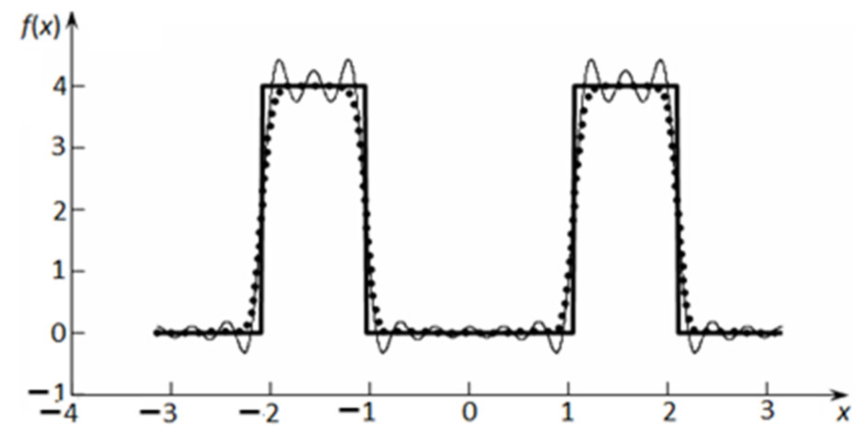
Example. Let a periodic function $f\left(x\right)$ with period 2π be defined as

$$f\left(x\right)=\left\{\begin{array}{c}0, \forall x\in \left(-\pi ,0\right];\\ x, \forall x\in \left(0,0=\pi \right].\end{array}\right.$$

Find the coefficients of the Fourier series

$$\begin{gathered} a_0=\frac{1}{\pi }\underset{-\pi }{\overset{\pi }{{\displaystyle \int }}}f\left(x\right)dx=\frac{1}{\pi }\left(\underset{-\pi }{\overset{0}{{\displaystyle \int }}}0dx+\underset{0}{\overset{\pi }{{\displaystyle \int }}}xdx\right)=\frac{1}{\pi }·\frac{{\pi }^2}{2}=\frac{\pi }{2}; \\ {a}_k=\frac{1}{\pi }\underset{-\pi }{\overset{\pi }{{\displaystyle \int }}}f\left(x\right)\sin kxdx=\frac{1}{\pi }\underset{0}{\overset{\pi }{{\displaystyle \int }}}x\sin kxdx=\frac{1}{\pi }\left(-\frac{x\cos kx}{k}{I}_0^{\pi }+\underset{0}{\overset{\pi }{{\displaystyle \int }}}\cos kxdx\right)=-\frac{1}{k}\cos kx; \\ {b}_k=\frac{1}{\pi }\underset{-\pi }{\overset{\pi }{{\displaystyle \int }}}f\left(x\right)\cos kxdx=\frac{1}{\pi }\underset{0}{\overset{\pi }{{\displaystyle \int }}}x\cos kxdx=\frac{1}{\pi }\left(\frac{x\sin kx}{k}{I}_0^{\pi }-\frac{1}{k}\underset{0}{\overset{\pi }{{\displaystyle \int }}}\sin kxdx\right)=\frac{1}{\pi k^2}(\cos kx-1). \end{gathered}$$

Then, the Fourier series for the original function will be written as follows

$$f\left(x\right)=\frac{\pi }{4}+\sin x-\frac{2}{\pi }\cos x-\frac{1}{2}\sin 2x+\frac{1}{3}\sin 3x-\frac{2}{9\pi }\cos 3x+\cdots .$$

The graphs of the original piecewise linear function (thickened line) and its approximations by several successive partial sums of the Fourier series (thin lines) on the segment [−π,π] are shown in Figure 2.

As you can see in Figure 2, the approximation error is large enough and, as will be shown in the next chapter, in the vicinity of the discontinuity points, even with an infinite increase in the number of terms in the Fourier series; the error, understood as the difference between the values of the original function and its approximation, does not tend to zero.

For an odd function, the coefficients of the Fourier series are found by the formulas

$$a_0=0; a_k=\frac{2}{\pi }\underset{0}{\overset{\pi }{\int }}f\left(x\right)\sin kxdx; b_k=0.$$

for an even function, these coefficients can be found as follows

$$a_0=\frac{2}{\pi }\underset{0}{\overset{\pi }{\int }}f\left(x\right)dx; a_k=0; b_k=\frac{2}{\pi }\underset{0}{\overset{\pi }{\int }}f\left(x\right)\cos kxdx.$$

In the case of a periodic function with a period of $2l$ by changing the variable, one can always go to a function with a period of 2π. In this case, the Fourier series for a function with a period $2l$ will have the form

$$f\left(x\right)=\frac{a_0}{2}+{\displaystyle \sum }_{k=1}^{\infty }\left(a_k\sin \frac{k\pi }{l}+b_k\cos \frac{k\pi }{l}\right),$$

where the coefficients are found by the formulas

$$a_0=\frac{1}{l}\underset{-l}{\overset{l}{\int }}f\left(x\right)dx; a_k=\frac{1}{l}\underset{-l}{\overset{l}{\int }}f\left(x\right)\sin \frac{k\pi }{l}xdx; b_k=\frac{1}{l}\underset{-l}{\overset{l}{\int }}f\left(x\right)\cos \frac{k\pi }{l}xdx.$$

If a piecewise-monotone non-periodic function is given, the values of which are of interest to us only on a certain interval $\left[a,b\right]$, then to expand this function in a Fourier series, we can use a periodic function with a period $2l\ge b-a$, which coincides with the original function on the interval $\left[a,b\right]$.

2.6. Function Approximation Using Splines

A spline is a function composed of parts of polynomials that form a basis [45,46,47,48,49]. The polynomials $1,x,x^2,\dots$ are usually taken as a basis. In the general case, the functions forming the basis may not be polynomials, but in the overwhelming majority of cases, so-called polynomial splines are constructed, the basic functions of which are precisely polynomials.

Some advantages of approximating the original function using splines can be pointed out:

1.

Stability of splines with respect to outliers and bursts;

2.

Good convergence of the approximation method;

3.

Ease of implementation on computers using well-developed mathematical methods such as the sweep method.

There are other advantages to this kind of approximation.

Let’s consider the basic idea of spline-function approximation.

Let the segment $\left[a,b\right]$ by points $x_0,x_1,x_2, \dots ,x_i,x_{i+1}, \dots , x_{n-1},x_n$, be divided into partial segments, so that

$$a=x_0<x_1<x_2<\dots <x_i<x_{i+1}<\dots <x_{n-1}<x_n=b.$$

It is said that a grid is given on the segment $\left[a,b\right]$. In addition, let $P_k$ be the set of all polynomials of degree at most $k,$ and $C^{\left(k\right)}\left[a,b\right]$ is the set of all continuous functions defined on the segment $\left[a,b\right]$ and having continuous derivatives on this segment up to the $k$-th order inclusive.

Definition 8.

The function $S_k\left(x\right)$ is called a spline of degree $k$ of a defect $d$ with a given grid if the following conditions are met:

1.

$S_k\left(x\right)\in P_k, \forall x\in \left[x_i, x_{i+1}\right], i=\overline{0,n-1};$

2.

$S_k\left(x\right)\in C^{\left(k-d\right)}\left[a,b\right]$.

Let some initial function $f\left(x\right)$ defined on the segment $\left[a,b\right]$ be given. A spline can be used to approximate this function by putting $S_k\left(x_i\right)=f\left(x_i\right), \forall i.$. In this case, the grid nodes are called approximation nodes.

Consider an example of drawing up a parabolic spline, that is, a spline of second degree.

Let there be a function $y\left(x\right)$, which at the nodes $x=0,1,2$ has the values 5, 2, 3, respectively.

For this function on the segment [0,2] we construct a spline of the form

$$S_2\left(x\right)=\left\{\begin{array}{c}{a}_1{x}^2+b_{1}x+c_1, \forall x\in \left[0,1\right);\\ a_2{x}^2+b_{2}x+c_2, \forall x\in \left[1,2\right].\end{array}\right.$$

From the condition $S_2\left(x_i\right)=y\left(x_i\right)$ we obtain

$$\left\{\begin{array}{c}{c}_1=5;\\ a_1+b_1+c_1=2;\\ a_2+b_2+c_2=2;\\ 4a_2+2b_2+c_2=3.\end{array}\right.$$

From the continuity condition for the first derivative, we find

$$2a_1+b_1=2a_2+b_2.$$

In total, we obtained five equations, but we also have six unknowns. Additional necessary equations are usually derived from some considerations, most often associated with boundary conditions. Putting, for example, $S_2^{″}\left(0\right)=0,$ we obtain the missing condition $b_1=0$.

Solving all the obtained equations in the system, we find the values of all coefficients $a_1=-3, a_2=7, b_1=0, b_2=-20, c_1=5, c_2=15$.

The desired spline will be written as follows

$$S_2\left(x\right)=\left\{\begin{array}{c}-3x^2+5, \forall x\in \left[0,1\right);\\ 7x^2-20x+15, \forall x\in \left[1,2\right].\end{array}\right.$$

The spline plot is shown in Figure 3.

Many practical examples, especially those related to mechanics, consider cubic splines, that is, splines of the third degree. Such splines allow not only the first derivative to be continuous, but also the second order derivative. In this case, it is possible to simulate the laws of motion with continuous speeds and accelerations. However, since we are primarily interested in piecewise linear functions, we will consider splines of the first degree, or, in other words, linear splines. The graphs of such splines will be continuous broken lines. For such splines, the following conditions will be met:

1.

$S_1\left(x\right)\in P_1, \forall x\in \left[x_i, x_{i+1}\right], i=\overline{0,n-1};$

2.

$S_1\left(x\right)\in C\left[a,b\right];$

3.

$S_1\left(x_i\right)=y\left(x_i\right), \forall i.$

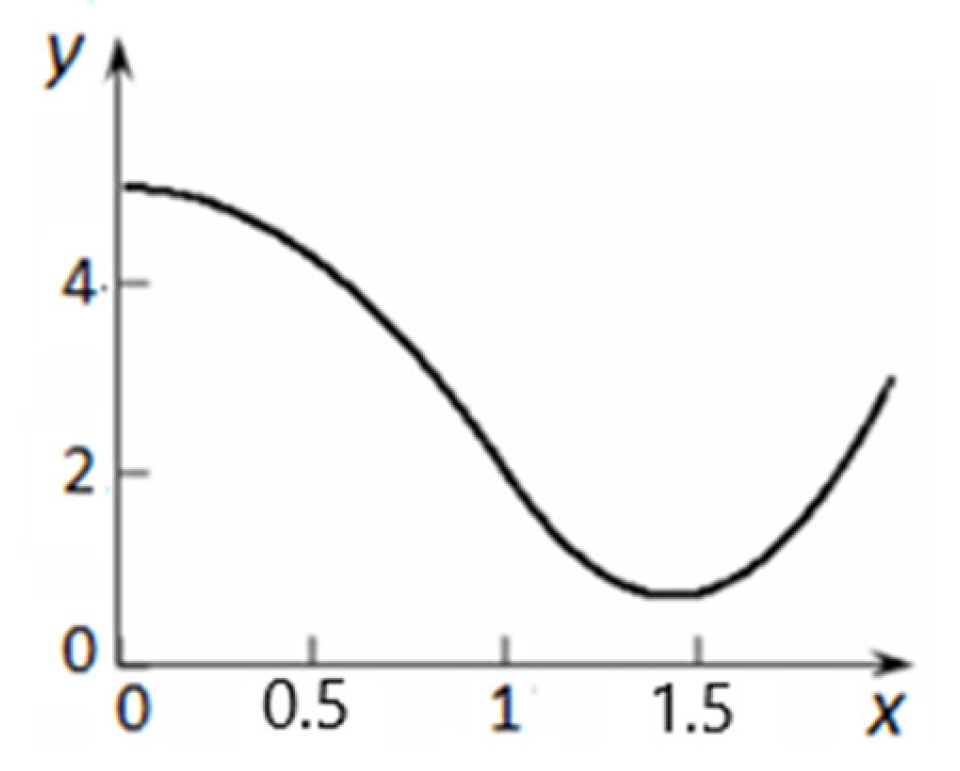
Example. The original function on the segment [0,10] is defined by the expression

$$y=\frac{5\sin x}{\sqrt[17]{2+\exp \left(3x\right)}}.$$

Taking the points at which $x=0,1,2,\dots ,10$, as the nodes of the approximation, we construct a linear spline, which will have the form

$$S\left(x\right)=\left\{\begin{array}{c}3.507x, x\in \left[0,1\right);\\ -0.314x+3.821, x\in \left[1,2\right);\\ -2.778x+8.749,x\in \left[2,3\right); \\ -2.284x+7.266, x\in \left[3,4\right);\\ -0.116x-1.404,x\in \left[4,5\right);\\ 1.499x-9.123, x\in \left[5,6\right);\\ 1.44x-9.123, x\in \left[6,7\right);\\ 0.251x-0.798, x\in \left[7,8\right);\\ -0.785x+7.483, x\in \left[8,9\right);\\ -0.8787x+8.402,x\in \left[9,10\right].\end{array}\right.$$

The graphs of the original function (solid line) and its approximating linear spline (dashed line) are shown in Figure 4.

The error in approximating the original functions using linear splines can be quite large. Nevertheless, in some cases, approximation by linear splines may be more preferable than approximation by splines of higher degrees, for example, due to simpler expressions for linear splines. In addition, the monotonicity of the values of the origin of the specified function for a linear spline is preserved, which may not be the case for splines of higher degrees.

To reduce the error, the number of nodal points can be increased, but at the same time, having a simple structure at each partial section, the linear spline acquires a cumbersome appearance as a whole, which is clearly seen in the example considered. In addition, already the first derivative for a linear spline is not continuous. This drawback often prevents linear spline functions from being used to solve practical problems. For example, the study of the dynamics of motion of various objects involves the use of velocities and accelerations, which are derivatives of the angles of rotation and displacement. Discontinuities in the functions for velocities and accelerations create uncertainties and inconsistencies between mathematical models and real processes. A way out of the situation can be the methods of approximation of piecewise linear splines, considered in the subsequent chapters and paragraphs of the review.

2.7. Least Squares Method: Linear Regression

The approximating function $F\left(x\right)$ by the least squares method [50,51] is determined from the condition of the minimum sum of squared deviations $\left({\xi }_i\right)$ of the calculated approximating function from a given array of experimental data. This criterion of the least squares method is written as the following expression:

$${\displaystyle \sum }_{i=1}^N{\xi }_i^2={\displaystyle \sum }_{i=1}^N{\left(F\left(x_i\right)-y_i\right)}^2 \to min,$$

where $F\left(x_i\right)$ are the values of the calculated approximating function $F\left(x\right)$ at the nodal points $x_i$; $y_i$ is a given array of experimental data at nodal points $x_i$.

This method can be useful when dealing with a large amount of information.

As an example, consider the method for determining the approximating function, which is given as a linear relationship [52]. In accordance with the least squares method, the condition for the minimum sum of squared deviations is written as follows:

$$S={\displaystyle \sum }_{i=1}^N{\xi }_i^2={\displaystyle \sum }_{i=1}^N{\left(a_0+a_1·x_i-y_i\right)}^2°\to min,$$

where $x_i,y_i$ are coordinates of nodal points of the table; $a_0,a_1$ are unknown coefficients of the approximating function, which is given as a linear dependence.

The necessary condition for the existence of a minimum of a function is the equality to zero of its partial derivatives with respect to unknown variables. Then, we obtain:

$$\left\{\begin{array}{c}\frac{\partial S}{\partial a_0}=2·{\displaystyle {\displaystyle \sum }_{i=1}^N}\left(a_0+a_1·x_i-y_i\right)=0;\\ \frac{\partial S}{\partial a_1}=2·{\displaystyle {\displaystyle \sum }_{i=1}^N}\left(a_0+a_1·x_i-y_i\right)·x_i=0.\end{array}\right.$$

After some transformations we have:

$$\left\{\begin{array}{c}{a}_0·N+a_1·{\displaystyle {\displaystyle \sum }_{i=1}^N}{x}_i={\displaystyle {\displaystyle \sum }_{i=1}^N}{y}_i;\\ a_0·{\displaystyle {\displaystyle \sum }_{i=1}^N}{x}_i+a_1·{\displaystyle {\displaystyle \sum }_{i=1}^N}{x}_i^2={\displaystyle {\displaystyle \sum }_{i=1}^N}{y}_i·x_i.\end{array}\right.$$

Solving the resulting system of linear equations, we find the coefficients of the approximating function:

$$\left\{\begin{array}{c}{a}_0=\frac{{{\displaystyle \sum }}_{i=1}^N{y}_i·{{\displaystyle \sum }}_{i=1}^N{x}_i^2-{{\displaystyle \sum }}_{i=1}^N\left(y_i·x_i\right)·{{\displaystyle \sum }}_{i=1}^N{x}_i}{N·{{\displaystyle \sum }}_{i=1}^N{x}_i^2-{\left({{\displaystyle \sum }}_{i=1}^N{x}_i\right)}^2};\\ a_1=\frac{N·{{\displaystyle \sum }}_{i=1}^N\left(y_i·x_i\right)-{{\displaystyle \sum }}_{i=1}^N{y}_i·{{\displaystyle \sum }}_{i=1}^N{x}_i}{N·{{\displaystyle \sum }}_{i=1}^N{x}_i^2-{\left({{\displaystyle \sum }}_{i=1}^N{x}_i\right)}^2}.\end{array}\right.$$

These coefficients are used to construct a linear approximating function according to the criterion of the minimum sum of squares of the approximating function from the given tabular values representing the experimental data.

Example. Suppose we have initial data (

Table 1. Initial data.

$x_i$	17.28	17.05	18.30	18.80	19.20	18.50
$y_i$	537	534	550	555	560	552

).

Using the above formulas, we find the pair of regression coefficients: $a_0=328.3, a_1=12.078$.

Then, the regression equation will take the form

$$y=12.078·x+328.3.$$

2.8. Hermite Interpolation

When constructing the Hermite interpolation polynomial, it is required that not only that its values coincide with the tabular data in the nodes, but also the values of its derivatives are in a certain order [53,54].

Let us now look at the nodes $x_i\in \left[a,b\right], i=0,1,\dots , m,$ among which there are no coinciding ones, the values of the function $f\left(x_i\right)$ and its derivatives $f^{\left(j\right)}\left(x_i\right),j=1,2, \dots , N_{i }-1$ up to $N_{i }-1$ order are given. In this case, the numbers $N_{i }$ are called the multiplicity of the node $x_i$. At each point $x_i$, thus, the following values $N_{i }$ are given: $f\left(x_i\right),f^{\prime }\left(x_i\right),f^{″}\left(x_i\right),\dots ,f^{\left(N_{i }-1\right)}\left(x_i\right).$ In total, the values $N_0+N_1+\dots +N_m$ are known on the entire set of nodes $x_0+x_1+\dots +x_m$, which makes it possible to raise the question of constructing a polynomial $H_n\left(x\right)$ of order $n=N_0+\dots +N_m-1,$ satisfying the requirements:

$$H_n^{\left(j\right)}\left(x_i\right)=f^{\left(j\right)}\left(x_i\right), i=0,1,\dots , m, j=1,2, \dots , N_{i }-1.$$

Such a polynomial is called the Hermite interpolation polynomial for the function $f\left(x\right)$. It is proved [] that the Hermite interpolation polynomial exists and is unique.

The construction of the Hermite polynomial in the general case for an arbitrary number of nodes and their multiplicity leads to rather cumbersome expressions and is rarely used. Therefore, we confine ourselves to one example.

Example. Construct the Hermite interpolation polynomial for the function $f\left(x\right)$ in the case when at all interpolation nodes $x_i\in \left[a,b\right], i=0,1,\dots , m,$ the values of the function $f\left(x_i\right)=f_i$ and its first derivative $f^{\prime }\left(x_i\right)=f_i^{\prime }$.

In this case $N_i=2,i=0,1,\dots , m,$ therefore, the degree of the polynomial $H_n\left(x\right)$ is $2m+1.$ We write the original polynomial in the form:

$$H_{2m+1}\left(x\right)={\displaystyle \sum }_{i=0}^m\left(f_i+{\alpha }_i\left(x-x_i\right)\right)·\frac{{\left(x-x_0\right)}^2·\dots ·{\left(x-x_{i-1}\right)}^2·{\left(x-x_{i+1}\right)}^2·\dots ·{\left(x-x_m\right)}^2}{{\left(x_i-x_0\right)}^2·\dots ·{\left(x_i-x_{i-1}\right)}^2·{\left(x_i-x_{i+1}\right)}^2·\dots ·{\left(x_i-x_m\right)}^2}.$$

When calculating the derivative of the polynomial $H_{2m+1}\left(x\right)$ at the node $x_i$, it should be taken into account that all terms of the sum, except for the term corresponding to the node itself, provide zero contribution to the derivative at this point, so we obtain

$$H_{2m+1}^{\prime }\left(x\right)=f_i·\left(\frac{2}{x_i-x_0}+\dots +\frac{2}{x_i-x_{i-1}}+\frac{2}{x_i-x_{i+1}}+\frac{2}{x_i-x_m}\right)+{\alpha }_i=f_i^{\prime }.$$

Therefore, we obtain ${\alpha }_i=f_i^{\prime }-2f_i{A}_i,$ where the numbers $A_i$ are determined by the formula

$$A_i=\frac{1}{x_i-x_0}+\dots +\frac{1}{x_i-x_{i-1}}+\frac{1}{x_i-x_{i+1}}+\frac{1}{x_i-x_m}.$$

Thus, the solution to this problem is the Hermite polynomial

$$H_{2m+1}\left(x\right)={\displaystyle \sum }_{i=0}^m\left(f_i+\left(f_i^{\prime }-2f_i{A}_i\right)·\left(x-x_i\right)\right)··\frac{{\left(x-x_0\right)}^2·\dots ·{\left(x-x_{i-1}\right)}^2·{\left(x-x_{i+1}\right)}^2·\dots ·{\left(x-x_m\right)}^2}{{\left(x_i-x_0\right)}^2·\dots ·{\left(x_i-x_{i-1}\right)}^2·{\left(x_i-x_{i+1}\right)}^2·\dots ·{\left(x_i-x_m\right)}^2}.$$

2.9. Lebesgue Functions and Lebesgue Constant in Polynomial Interpolation

The Lebesgue constant is a valuable numerical tool for linear interpolation because it provides a measure of how close the interpolation of a function is to the best polynomial approximation of a function. Many publications [55,56,57,58,59] have been devoted to finding optimal interpolation points in the sense that these points lead to the minimum Lebesgue constant for interpolation problems on the interval [−1,1].

Definition 9.

Let ${\Omega }_n={\left\{x_i\right\}}_{i=1}^n$ be a grid on $\left[a,b\right]$.

Function ${\Lambda }_n\left(x\right)={\Lambda }_n\left(x, x_1,x_2,\dots ,x_n\right)={\sum }_{i=1}^n\left|l_i\left(x\right)\right|$ is called the Lebesgue function, and the Lebesgue constant is the number

$${\Lambda }_n={\Lambda }_n\left(x_1,x_2,\dots ,x_n\right)=\underset{x\in \left[a,b\right]}{\max }{\Lambda }_n\left(x, x_1,x_2,\dots ,x_n\right).$$

Here $l_1\left(x\right), l_2\left(x\right),\dots , l_n\left(x\right)$ is some basis in the linear (vector) space of functions of dimension $n$.

The statements are true [59]:

• $1\le {\Lambda }_n\left(x\right)\le {\Lambda }_n$ for any $x\in \left[a,b\right]$.
• The value of ${\Lambda }_n$ does not depend on $\left[a,b\right]$, but depends only on the relative position of the nodes on it.

Let us pose the question: to what extent is the method of interpolation of a function by an algebraic polynomial inferior in accuracy to the best possible method of approximating a function by an algebraic polynomial of the same degree?

Let $P_{n-1 }$ be an algebraic polynomial, an approximation of the function $f$, obtained by some method. Thus, each method has its own polynomial $P_{n-1 }$. The value $\left|f\left(x\right)-P_{n-1}\left(x\right)\right|$ determines the approximation error at a point $x\in \left[a,b\right]$, and the number ${\Vert f-P_{n-1}\Vert }_{\infty }=\underset{x\in \left[a,b\right]}{\max }\left|f\left(x\right)-P_{n-1}\left(x\right)\right|$ is the maximum error of this method.

Definition 10.

An algebraic polynomial $L_{n-1 }$ is called a polynomial of best uniform approximation if ${\Vert f-L_{n-1}\Vert }_{\infty }=\underset{P_{n-1}}{\min }{\Vert f-P_{n-1}\Vert }_{\infty }.$ The solution to this problem exists and is uniquely determined. The value $E_n\left(f\right)={\Vert f-L_{n-1}\Vert }_{\infty }$ is called the error of the best uniform approximation.

Let’s make the following remarks:

• If $F_{n-1}$ is an approximation of $f$ obtained by some method (for example, $F_{n-1}$ is an interpolation polynomial), then ${\Vert f-F_{n-1}\Vert }_{\infty }\ge E_n\left(x\right)$.
• $E_n\left(x\right) \to 0$ as $n\to \infty$ for any function $f$ continuous on $\left[a,b\right]$. This follows directly from the Weierstrass’ theorem.

Theorem 6.

The estimates $E_n\left(f\right)\le {\Vert f-R_{n-1}\Vert }_{\infty }\le \left(1+{\Lambda }_n\right)E_n\left(f\right)$ are valid.

Proof. 

Let $L_{n-1 }$ be a polynomial of the best uniform approximation of $f$. Since the interpolation polynomial is unique, $L_{n-1 }\left(x\right)={\sum }_{i=1}^n{L}_{n-1 }\left(x_i\right)l_i\left(x\right).$ Therefore,

$$\begin{array}{ll}\left|f\left(x\right)-R_{n-1}\left(x\right)\right|& =\left|f\left(x\right)-L_{n-1 }\left(x\right)+L_{n-1 }\left(x\right)-R_{n-1}\left(x\right)\right|\\ & \le \left|f\left(x\right)-L_{n-1 }\left(x\right)\right|+{\displaystyle {\displaystyle \sum }_{i=1}^n}\left|L_{n-1 }\left(x_i\right)-f\left(x_i\right)\right|l_i\left(x\right)\\ & \le \left(1+{\Lambda }_n\left(x\right)\right){\Vert f-L_{n-1}\Vert }_{\infty }\le \left(1+{\Lambda }_n\right)E_n\left(f\right).\end{array}$$

□

The lower estimate is valid by the definition of $E_n\left(f\right)$. It follows from the upper estimate that the interpolation polynomial $R_{n-1}\left(x\right)$ is less accurate than the best uniform approximation by a maximum of $1+{\Lambda }_n$ times in accuracy.

Let’s pose the second question: how sensitive is the interpolation polynomial to the error in setting the function?

Let the approximate values $\tilde{f}\left(x_i\right)$ be known at the interpolation nodes instead of the exact values of $f\left(x_i\right)$ with an error $ϵ\left(x_i\right)$ not exceeding $\epsilon :\left|ϵ\left(x_i\right)\right|=\left|f\left(x_i\right)-\tilde{f}\left(x_i\right)\right|\le \epsilon .$ Thus, instead of $R_{n-1}\left(x\right)$ the perturbed polynomial ${\tilde{R}}_{n-1}\left(x\right)$ will be constructed from the values of $\tilde{f}\left(x_i\right)$. Of practical interest is the deviation of ${\tilde{R}}_{n-1}$ from $f$.

Theorem 7.

The estimate is $\left|f\left(x\right)-{\tilde{R}}_{n-1}\left(x\right)\right|\le \left|f\left(x\right)-R_{n-1}\left(x\right)\right|+\epsilon {\Lambda }_n$.

Proof. 

Obviously,

$$\left|R_{n-1}\left(x\right)-{\tilde{R}}_{n-1}\left(x\right)\right|=\left|{\displaystyle \sum }_{i=1}^n\left(f\left(x_i\right)-\tilde{f}\left(x_i\right)\right)l_i\left(x\right)\right|\le \epsilon {\Lambda }_n.$$

Therefore,

$$\left|f\left(x\right)-{\tilde{R}}_{n-1}\left(x\right)\right|\le \left|f\left(x\right)-R_{n-1}\left(x\right)\right|+\left|R_{n-1}\left(x\right)-{\tilde{R}}_{n-1}\left(x\right)\right|\le \left|f\left(x\right)-R_{n-1}\left(x\right)\right|+\epsilon {\Lambda }_n.$$

□

It follows from estimate that the larger ${\Lambda }_n$, the more sensitive the interpolation procedure to the error in setting the function.

Important conclusions follow from the estimates obtained [59]:

1.

The smaller the Lebesgue constant ${\Lambda }_n$, and the smoother the function, the better both in terms of accuracy and the sensitivity of interpolation to the error of setting the function;

2.

If the sequence of grids ${\Omega }_n={\left\{x_i\right\}}_{i=1}^n$ satisfies the condition ${\Lambda }_n{E}_n\left(f\right)\to 0$ as $n\to \infty$, then $\left|f\left(x\right)-R_{n-1}\left(x\right)\right|\to 0$ as $n\to \infty$ uniformly in $x$ (in this case one speaks of the convergence of the interpolation process);

3.

During calculations, the following picture can be observed: the error $\left|f\left(x\right)-{\tilde{R}}_{n-1}\left(x\right)\right|$ as $n$ increases, it first decreases and then begins to increase.

The value of ${\Lambda }_n$ depends on the choice of nodes ${\Omega }_n$.

A detailed consideration of issues related to the significance of the Lebesgue constant, moduli of smoothness, selection of optimal nodes, weighted polynomial interpolation is given in fundamental works [1,2,3,4].

3. New Methods of Approximation of Piecewise-Linear and Generalized Functions

This section of the review describes new methods for approximating piecewise-linear functions, especially, piecewise constant functions, and generalized functions, a comparative analysis of the proposed and existing methods for approximating such functions by analytical dependences based on Fourier series is carried out. In addition, the issues of convergence and error of the proposed methods are studied, numerous examples and applications are considered.

The general idea of using a repeating procedure, which gives a more accurate result with each subsequent application, is the basis, for example, of the mathematical theory of deep learning. Deep learning is a type of machine learning using multi-layer neural networks that learn on their own on a large dataset. Artificial intelligence with deep learning itself finds an algorithm for solving the original problem, learns from its mistakes, and after each iteration of training gives a more accurate result.

3.1. Disadvantages of Approximating Piecewise Linear Functions by Fourier Series

To simplify calculations, when working with piecewise linear and generalized functions, in many cases they resort to approximation methods. Replacing piecewise linear functions with more regular $C^k$ functions allows you not to worry about tracking and matching the values of process variables at the boundaries of the sections, which greatly simplifies the calculations. In some cases, algebraic polynomials are used to approximate piecewise linear functions. Another of the most widely used methods for approximating piecewise linear functions is the expansion of these functions using Fourier series $f={\sum }_{k=1}^{\infty }{c}_k{\phi }_k$, where $\left\{{\phi }_1,{\phi }_2, \dots ,{\phi }_n, \dots \right\}$ is orthogonal system in the functional Hilbert space $L_2\left[-\pi ,\pi \right]$ of measurable functions with Lebesgue integrable squares,$f\in L_2\left[-\pi ,\pi \right], c_k=\left(f,{\phi }_k\right)/{\Vert {\phi }_k\Vert }^2$. The trigonometric system of 2π-periodic functions $\left\{1,\sin nx,\cos nx, n\in N\right\}$ is often taken as the orthogonal system.

As for the approximation of continuous functions by polynomials or Fourier series, we can discuss the uniform convergence of the approximating functions based on the Weierstrass theorems.

However, for discontinuous piecewise linear functions, the Weierstrass theorems do not hold. Therefore, when approximating such functions, problems may arise that cause negative consequences when solving applied problems. For example, the use of Fourier series, along with positive properties, has certain disadvantages. With a relatively small number of terms in the Fourier series used for the expansion of piecewise-linear functions, the approximating function has a pronounced wavy character even within one rectilinear section of the piecewise-linear function, which leads to a sufficiently large approximation error. to approximate continuous functions. Curves 1 and 2 in Figure 5 illustrate this drawback.

Moreover, even for a large number of terms in the expansion using the Fourier series, there are characteristic jumps of the approximating function in the vicinity of the discontinuity points $O_{\delta }(x_0)$ of the original function. For such points $\underset{x\in O_{\delta }(x_0)/\left\{x_0\right\}}{\sup }\left|f(x)-S_n(x)\right|\underset{n\to \infty }{\to }A\ne 0$, where $S_n(x)$ is the partial sum of the Fourier series [60].

For example, for the function

$$f_0(x)=\mathrm{sign}(\sin x)$$

(1)

with rectangular pulses, the point $x=\pi /m$, where $m=2[(n+1)/2], [A]$ is the integer part of the number $A$, is the maximum point of the partial sum $S_n(f_0)$ of the trigonometric Fourier series [61], moreover $S_n\left(f_0,\pi /m\right) \underset{\hspace{1em}n\to \infty \hspace{1em}}{\to } \frac{2}{\pi }{\int }_0^{\pi }\frac{\sin t}{t}dt\approx 1.17898$. That is, the magnitude of the absolute error $\left|f_0\left(\pi /m\right)-\underset{n\to \infty }{\lim }{S}_n\left(f_0, \pi /m\right)\right| > 0$.178, and the relative error is more than 17%, regardless of the number of terms in the partial sum of the Fourier series. Notice, that $x=\pi /m \underset{n\to \infty }{\to } 0+0$.

In Figure 5, curve 3 corresponds to the graph of the approximating function $f_n\left(x\right)={\sum }_{n=1}^{20}{c}_n{\phi }_{n }$ and illustrates the increased approximation error in the vicinity of the discontinuity points of the original Function (1). This is the manifestation of the so-called Gibbs effect, and with an increase in the number of harmonics, the Gibbs effect does not disappear, which leads to extremely negative consequences of using the approximating function. Figure 6 shows a graph of the partial sum $S_{20}\left(f_0\right)$ of the trigonometric series on the segment [−π,π], illustrating the manifestation of the Gibbs effect.

The most unpleasant thing is that the Gibbs effect is general in nature, it manifests itself for any function $f\in L_2[a, b]$, that has bounded variation on a segment $[a, b]$, with an isolated breakpoint $x_0\in (a, b)$. For such functions, the following condition is satisfied [61]

$$\underset{n\to \infty }{\lim }{S}_n(f, x_0+\pi /m)=f(x_0+0)+\frac{d}{2}\cdot \left(\frac{2}{\pi }{\displaystyle \underset{0}{\overset{\pi }{\int }}\frac{\sin t}{t}dt-1}\right),$$

where $d=f(x_0+0)-f(x_0-0)$.

Let us show that the absolute $\Delta =\Delta (x)$ and conditional $\delta =\delta (x)$ approximation errors in the vicinity of the discontinuity points can be arbitrarily large.

Really,

$$\begin{array}{l}\underset{n\to \infty }{\lim }\Delta (x_0+\pi /m)=\underset{n\to \infty }{\lim }\left|S_n(f,x_0+\pi /m)-f(x_0+\pi /m)\right|=\left|\underset{n\to \infty }{\lim }{S}_n(x_0+\pi /m)-\underset{n\to \infty }{\lim }f(x_0+\pi /m)\right|\\ =\left|f(x_0+0)+\frac{d}{2}\cdot \left(\frac{2}{\pi }{\displaystyle \underset{0}{\overset{\pi }{\int }}\frac{\sin t}{t}dt-1}\right)-f(x_0+0)\right|=\left|\frac{d}{2}\cdot \left(\frac{2}{\pi }{\displaystyle \underset{0}{\overset{\pi }{\int }}\frac{\sin t}{t}dt-1}\right)\right|=\Delta (d).\end{array}$$

For each $d$ there exists a function $f=f_{d }$ satisfying the previous conditions. The property $\Delta \left(d\right) \to +\infty$ has to be understood in this way. The function $\Delta (d)$ is infinitely large since

$$\forall M>0 \exists \hspace{0.17em}d=d^{\ast }(M)>0 \forall d: \left|d\right|>d^{\ast }\Rightarrow \Delta (d^{\ast })=\left|\frac{d^{\ast }}{2}\cdot \left(\frac{2}{\pi }{\displaystyle \underset{0}{\overset{\pi }{\int }}\frac{\sin t}{t}dt-1}\right)\right|>M.$$

As $d^{\ast }$ you can take, for example, $\left[2M\pi /\left(2{\displaystyle \underset{0}{\overset{\pi }{\int }}\frac{\sin t}{t}dt-\pi }\right)\right]+1$.

For the relative error $\delta (x)=\Delta (x)/\left|f(x)\right|$ the proof is similar. Moreover, even with a fixed value $d\in \mathit{R}$$(d\ne 0)$ for any $M>0$ you can choose a function $f(x)\in L_2[a,b]$, for which $\delta (x_0+0,d)=\Delta (x_0+0,d)/\left|f(x_0+0)\right|>M$. As such a function, for example, one can take a function $f,$ or which $\left|f(x_0+0)\right|<\Delta (x_0+0,d)/M, f(x_0+0)\ne 0$.

Note that even on the set of continuous functions $C [-\pi , \pi ]$ the Fourier series, as is known [31], does not yet have to converge at every point.

The existence of the Gibbs effect leads to extremely negative consequences of using a partial sum of a trigonometric series as an approximating function for solving problems of mathematical modeling, for example, when studying periodic movements of technical systems, distortions in signal transmission, etc.

The approximation error is especially striking when using Fourier series for generalized functions, for example, δ—function or, in other words, Dirac function. This function is widely used to describe the density of a point mass, the density of a point charge, quantum theory, concentrated loads, instantaneous impulse processes, shock effects, the intensity of a point heat source, diffusion processes in semiconductors, etc.

Generalized functions were introduced in connection with the problems of physics and mathematics that appeared in the twentieth century and required a new understanding of the concept of a function. Generalized singular functions are very different from regular functions. It is known that the δ—function is not a function in the usual sense of this word; rather, it is determined by a functional, and informally by the expression

$$\delta (x)=\left\{\begin{array}{l}+\infty , x=0, \\ 0, \forall x\ne 0,\end{array}\right.$$

moreover ${\displaystyle \underset{-\infty }{\overset{+\infty }{\int }}\delta (x)dx=1}$.

Generalized functions were introduced in mathematics by Sobolev and Schwartz [62,63,64,65]. Generalized functions have become a key tool in much of PDE theory and form a huge part of analysis.

Let us provide a mathematically more precise definition of a generalized function.

Definition 11.

A generalized function in the sense of Sobolev-Schwartz is any linear continuous functional on the space of basic functions [23].

Thus: (1) the generalized function $f$ is a functional on the set of basic functions $D$ [23], that is, each support of the piecewise continuous function [23] $\phi \in D$ is associated with a (complex) number $\left(f,\phi \right)$; (2) a generalized function $f$ is a linear functional on $D$, that is, if $\phi ,\psi \in D$ and $\lambda ,\mu$ are complex numbers, then $\left(f,\lambda \phi +\mu \psi \right)=\lambda \left(f,\phi \right)+\mu \left(f,\psi \right);$ (3) the generalized function $f$ is a continuous functional on $D$, that is, if ${\phi }_k\to \phi , k\to \infty$ in $D$, then $\left(f,{\phi }_k\right)\to \left(f,\phi \right), k\to \infty$.

A very intuitive graph of δ—function is shown in Figure 7.

For the convenience of using analytical research methods, the delta function is decomposed into a Fourier series.

We introduce a sequence of step functions of the form

$${\delta }_n(x)=\left\{\begin{array}{l}n/2, \forall x\in [-1/n, 1/n],\\ 0, \forall x\notin [-1/n, 1/n].\end{array}\right.$$

The functions of this sequence have graphs corresponding to the graph of the step function shown in Figure 8.

It is easy to see that for any $n$ the area of the figure under the graph of such a step function is equal to one.

For the function, the graph of which is shown in Figure 8, we find the values of the coefficients of the Fourier series on the segment [−π,π]:

$$a_0=\frac{1}{\pi }{\displaystyle \underset{-\pi }{\overset{+\pi }{\int }}{\delta }_n(x)dx=}\frac{1}{\pi }{\displaystyle \underset{-1/n}{\overset{1/n}{\int }}\frac{n}{2}dx=}\frac{1}{\pi };$$

$$\begin{gathered} a_k=0, \mathrm{due} \mathrm{to} \mathrm{the} \mathrm{parity} \mathrm{of} \mathrm{the} \mathrm{function}; \\ {b}_k=\frac{1}{\pi }{\displaystyle \underset{-\pi }{\overset{\pi }{\int }}{\delta }_n(x)\cos kxdx}=\frac{1}{\pi }{\displaystyle \underset{-1/n}{\overset{1/n}{\int }}\frac{n}{2}\cos kxdx=\frac{1}{\pi }\cdot \frac{n}{2}\cdot \frac{2}{n}\cos (k{x}^{\ast })=\frac{\cos (k{x}^{\ast })}{\pi }}, \\ {x}^{\ast }\in [-1/n, 1/n], \end{gathered}$$

by virtue of the theorem on the mean value of a definite integral.

Equalities with $\delta \left(x\right)$ have to be meant in the sense of limits of sequences distributions.

The equalities with δ(x) have to be meant in the sense of limits of sequences distributions. In the theory of generalized functions, the limit of a sequence of distributions is the distribution that sequence approaches. The distance, suitably quantified, to the limiting distribution can be made arbitrarily small by selecting a distribution sufficiently far along the sequence. This notion generalizes a limit of a sequence of functions; a limit as a distribution may exist when a limit of functions does not.

Given a sequence of distributions $f_n$, its limit $f$ is the distribution given by $f\left(\phi \right)=\underset{n\to \infty }{\lim }{f}_n\left(\phi \right)$ for each test function $\phi$, provided that distribution exists.

Since the delta function $\delta (x)=\underset{n\to \infty }{\lim }{\delta }_n(x)$ and noticing that $x^{\ast }\underset{n\to \infty }{\to }0$, we find $b_k=\frac{1}{\pi }$.

Consequently, the expansion of the delta function in a Fourier series on the interval $[-\pi , \pi ]$ has the form

$$\delta (x)=\frac{1}{2\pi }+\frac{1}{\pi }{\displaystyle \sum _{k=1}^{\infty }\cos (kx).}$$

For a finite series, we have an approximate relation

$$\delta (x)\approx \frac{1}{2\pi }+\frac{1}{\pi }{\displaystyle \sum _{k=1}^n\cos (kx).}$$

This approximate equality is only informal because the point value $\delta \left(x\right)$ has no meaning in Sobolev-Schwartz theory. Generalized function can be considered as set-theoretical maps (in a non-Archimedean ring of scalars) [24].

The graph of the approximation of the delta function by the Fourier series is shown in Figure 9.

Comparison of the graphs (Figure 7 and Figure 9) shows that even with a significant number of harmonics (in our case n = 1000), the approximation error is very large. The minimum value of the constructed approximation is negative and is −69.182. Moreover, with an infinite increase in the number of terms in the approximating Fourier series, the minimum value of its sum tends to −∞ (Figure 10), which fully corresponds to the assertion proved in this section about the possible infinitely large error in approximation using the Fourier series.

The existence of the Gibbs effect in the approximation of functions by trigonometric expressions also makes the proof of some important theorems critical. In particular, in the theory of signal transmission, the classical sampling Nyquist-Shannon-Kotelnikov theorem is widely used. When proving the theorem [66] to approximate functions, it uses the so-called integral sine determined by the expression.

On the basis of the integral sine Kotelnikov V.A. to prove the theorem [66] builds a function $Si(T(\omega +{\omega }_1))-Si(T(\omega -{\omega }_1))$, where $\omega$ is argument, $T, {\omega }_1$ are some parameters. At the same time, he claims that with increasing $T$ this function tends to the limits shown in Figure 11a, that is, we quote literally, is equal to zero at $\omega >{\omega }_1$ and equal to $\pi$ at $\omega <{\omega }_1$.

In fact, this is not the case. The graph of the limiting function will have the form shown in Figure 11b. That is, for any, even arbitrarily large but finite values of the parameter $T$, there will always be those $\omega <{\omega }_1$, for which the values of the function constructed by Kotelnikov will be different from $\pi$, and there will always be those $\omega >{\omega }_1$, for which its values will be different from zero. Moreover, it is important to note that the indicated difference with increasing $T$ does not tend to zero, but tends to some number other than zero, approximately equal to 0.281, that is, constituting a sufficiently large value. Therefore, the classical sampling Nyquist-Shannon-Kotelnikov theorem requires a careful revision.

In the practice of creating images, the noted errors lead to a speckle effect, which manifests itself in the spotting of such images, their increased graininess (Figure 12). The speckle effect is the result of the interference of many waves of the same frequency, having different phases and amplitudes, which add up to the resulting wave, the amplitude and, therefore, the intensity of which changes randomly. It seems to the viewer that the image is covered with frequent, small spots, which, of course, degrades the quality of these images. Such disadvantages in signal transmission led to signal distortions, which can be significant.

The described shortcomings clearly indicate the need to develop new, more efficient methods for approximating piecewise linear functions.

3.2. Description of New Methods of Approximation of Piecewise-Linear Functions and Their Convergence

To eliminate the noted shortcomings, S. Aliukov [5,6,11,14,16] proposed new methods for approximating piecewise-linear functions, based, like the Fourier series, on the use of trigonometric expressions, but in the form of recursive functions.

To explain these methods, consider, for example, step Function (1) in more detail. This function is often used for an example of the application of Fourier series and therefore it is convenient to take this function for a comparative analysis of the traditional Fourier series expansion and the proposed method.

The expansion of Function (1) in a Fourier series has all the above-described disadvantages. To eliminate them, it is proposed to approximate the original step function by a sequence of recursive periodic functions

$$\left\{f(x)n \left|{ f}_n(x)=\sin \left((\pi /2)\cdot f_{n-1}(x)\right), f_1(x)=\sin x; n-1\in \mathit{N}\right.\right\}\subset C^{\infty }[-\pi ,\pi ]$$

(2)

The graphs of the original function (thickened line) and its five successive approximations in this case have the form (Figure 13).

As you can see, even with relatively small values when using the iterative procedure (2), the graph of the approximating function approximates the original Function (1) quite well. In this case, the approximating functions obtained using the proposed method are free from the drawbacks of expansion in Fourier series. The Gibbs effect is completely absent.

Let us note some features of the proposed approximating iteration procedure.

Note that the functions $f_n(x)$ and $f_0(x)$ are odd and periodic with a period $2\pi$. The functions $f_n(x+\pi /2)$ and $f_0(x+\pi /2)$ are periodic even. Therefore, it is sufficient to consider the sequence of approximating functions (2) on an interval $\left[0, \pi /2\right]$.

Theorem 8.

The sequence of functions $f_n(x)$ converges to the original function $f_0(x)$, and the convergence is pointwise, but not uniform.

Proof. 

At points $x=0$ and $x=\mathit{\pi }/2$ we have $f_n(x)-f_0(x)=0, \forall n\in \mathit{N}$. Therefore, at these points $f_n(x)\underset{n\to \infty }{\to }{f}_0(x)$.

Since $\sin x>(2/\pi )\cdot x, \forall x\in (0, \pi /2)$, then the condition $f_n(x)=\sin \left((\pi /2)\cdot f_{n-1}(x)\right)>f_{n-1}(x)>\dots >f_1(x)>0$ is satisfied for any $x\in (0, \pi /2)$. Then, the sequence $f_n(x), \forall x\in (0, \pi /2)$ is positive, increasing, and bounded, and therefore has a finite limit, which we denote by $\underset{n\to \infty }{\lim }f(x)n=A\in \mathit{R}$. We obtain $A=\underset{\mathit{n}\to \infty }{\lim }\sin ((\pi /2)\cdot f_{n-1}(x))=\sin ((\pi /2)\cdot \underset{\mathit{n}\to \infty }{\lim }{f}_{\mathit{n}-1}(x))=\sin ((\pi /2)\cdot A)$, whence we find that $A=0$ or $A=1$. Since the sequence is positive and increasing, then $A=1=f_0(x)$. Then, on the considered interval $f_n(x)\underset{n\to \infty }{\to }{f}_0(x)$. Taking into account the previously made conclusion about the convergence of the sequence at the points $x=0$ and $x=\pi /2$, we conclude that $f_n(x)\underset{n\to \infty }{\to }{f}_0(x), \forall x\in [0, \pi /2]$. This convergence is only pointwise and not uniform since the function $f_0(x)$ is not continuous on the segment $\left[0, \pi /2\right]$. □

Theorem 9.

In the space of measurable functions $L_1[0,\pi /2]$ and in the Hilbert space $L_2[0,\pi /2]$ the sequence of approximating functions $f_n(x)$ converges in the norm to the original function $f_0(x)$.

Proof. 

We introduce a sequence of minorants with respect to a sequence $f_n(x)$ of functions

$$\left\{{\eta }_n(x) \left| {\eta }_n(x)=(2/\pi )\cdot \mathrm{arctg}(n\pi ); n\in \mathit{N}\right.\right\}\subset C^{\infty }[0,\pi /2].$$

It can be shown that $f_n(x)\ge {\eta }_n(x), \forall n\in \mathit{N}, \forall x\in [0, \mathit{\pi }/2]$. Note that the measure of the set of discontinuity points of the function $f_0(x)$ is equal to zero. Then, taking into account the non-negative sign and boundedness of the functions $f_n(x)$ and ${\eta }_{\mathit{n}}(x)$ and on the segment under consideration, in space $L_1[0, \pi /2]$ we obtain

$$\left|\left|f_0(x)-f_n(x)\right|\right|={\displaystyle \underset{0}{\overset{\pi /2}{\int }}(1-f_n(x))dx}\le {\displaystyle \underset{0}{\overset{\pi /2}{\int }}(1-{\eta }_n(x))dx}=\frac{\pi }{2}-\mathrm{arctg}\frac{\pi n}{2}+\frac{1}{\pi n}\cdot \ln \left(1+{(\pi n)}^2/4\right).$$

Since $\underset{n\to \infty }{\lim }\left(\frac{\pi }{2}-\mathrm{arctg}\frac{\pi n}{2}+\frac{1}{\pi n}\cdot \ln \left(1+{(\pi n)}^2/4\right)\right)=0$, then $\left|\left|f_0(x)-f_n(x)\right|\right|\underset{n\to \infty }{\to }0$.

Similarly, one can prove that the sequence $f_n(x)$ converges in the norm to a function $f_0(x)$ in the space $L_2[0,\pi /2]$. □

Thus, the sequence of approximating functions $f_n(x)$ in spaces $L_1[-\pi ,\pi ]$ and $L_2[-\pi ,\pi ]$ is fundamental. In space $C[-\pi ,\pi ]$ the sequence $f_n(x)$ is not fundamental.

The function $f_1(x)$ will be called initial (or angular). Instead of sine, we can use another (not necessarily periodic) function as an initial function. Note that when using the iterative procedure (2) and under the condition $\left|f_1(x)\right|<2$ we obtain $\underset{n\to \infty }{\lim }{f}_n(x)=\mathrm{sign}(f_1(x))$. In this case, any step function can be approximated. Indeed, for the step function

$$f(x)=\left\{\begin{array}{l}h, x\in (x_1,x_2),\\ 0, x\notin (x_1,x_2)\end{array}\right.$$

(3)

take the initial function in the form $f_1(x)=\exp (1-{(ax+b)}^2)-1$. From the condition $f_1(x_1)=f_1(x_2)=0$ we find $a=2/(x_1-x_2); b=(x_1+x_2)/(x_2-x_1)$. For these values of the coefficients $a$ and $b$ the sequence

$$\left\{f_n(x) \left| f_n(x)=(h/2)\cdot (1+\sin {\phi }_{\mathit{n}}(x)), {\phi }_{\mathit{n}}(x)=(\pi /2)\cdot \sin {\phi }_{\mathit{n}-1}, {\phi }_1(x)=(\pi /2)\cdot f_1(x), n-1\in \mathit{N} \right.\right\}$$

converges to the step function $f(x)$. Then, any step function with values $h_i$ on the intervals $(x_{1i},x_{2i})$ can be approximated by the sum of similar sequences ${\displaystyle \sum _{\mathit{i}=1}^{\mathit{k}}{\left\{f_n(x)\right\}}_{\mathit{i}}}$.

The proved Theorem 2 is of a general nature and is valid for an arbitrary step function. Therefore, for example, an arbitrary periodic step function can be represented as a linear combination $f\left(x\right)={\sum }_{i=1}^k{h}_i·f_{0i}\left(x\right), h_i\in R,$ shifted in phase and along the ordinate axis functions $f_{0i}\left(x\right)=\mathrm{sign}\left(\sin \left(l_{i}x-x_i\right)\right),l_i,x_i\in R$. According to the proved theorem, in the spaces $L_1\left[-\pi ,\pi \right]$ and $L_2\left[-\pi ,\pi \right]$ we have the convergence $\Vert f_{0i}\left(x\right)-f_{ni}\left(x\right)\Vert \underset{n\to \infty }{\to }0$,$\forall i$, therefore the function $f_n\left(x\right)={\sum }_{i=1}^k{h}_i·f_{ni}\left(x\right)$ converges in the norm to the function $f\left(x\right)$, since

$$\Vert f\left(x\right)-f_n\left(x\right)\Vert =\Vert {\displaystyle \sum }_{i=1}^k{h}_i·f_{0i}\left(x\right)-{\displaystyle \sum }_{i=1}^k{h}_i·f_{ni}\left(x\right)\Vert \le {\displaystyle \sum }_{i=1}^k\left|h_i\right|·\Vert f_{0i}\left(x\right)-f_{ni}\left(x\right)\Vert \underset{n\to \infty }{\to }0.$$

3.3. Approximation Error

To estimate the error of approximation (2), we use the relation

$${\phi }_n\left(x\right)\le f_n\left(x\right)\le {\psi }_n\left(x\right)$$

(Figure 14), where

$${\psi }_n\left(x\right)={\left(\pi /2\right)}^{n-1}·x, x\in \pi /2, n\in N.$$

Functions ${\phi }_n\left(x\right)$ and ${\psi }_n\left(x\right)$ are constructed from the condition of equality of derivatives at zero ${\phi }_n^{\prime }\left(x\right)={\psi }_n^{\prime }\left(x\right)=f_n^{\prime }\left(x\right)$, which allows one to obtain a narrow interval for estimating the approximation error.

In space $L_1\left[0,\pi /2\right]$ the estimates for the absolute and relative errors are, respectively

$$\frac{{\left(2/\pi \right)}^{n-1}}{2}\le {\Vert f_n\left(x\right)-f_0\left(x\right)\Vert }_{L_1\left[0,\frac{\pi }{2}\right]}\le {\left(\frac{2}{\pi }\right)}^{n-1}·\left(1-\exp \left(-{\left(\frac{\pi }{2}\right)}^n\right)\right);$$

$$\frac{{\left(2/\pi \right)}^n}{2}\le \frac{\left({\Vert f_n\left(x\right)-f_0\left(x\right)\Vert }_{L_1\left[0,\frac{\pi }{2}\right]}\right)}{\left(\frac{\pi }{2}\right)}\le {\left(\frac{2}{\pi }\right)}^n·\left(1-\exp \left(-{\left(\frac{\pi }{2}\right)}^n\right)\right).$$

For space $L_2\left[0, \pi /2\right]$, these estimates take, respectively, the form

$${\left({\left(2/\pi \right)}^{n-1}/3\right)}^{1/2}\le {\Vert f_n\left(x\right)-f_0\left(x\right)\Vert }_{L_2\left[0,\frac{\pi }{2}\right]}\le {\left({\left(\frac{2}{\pi }\right)}^{n-1}·\frac{\left(1-\exp \left(-2{\left(\frac{\pi }{2}\right)}^n\right)\right)}{2}\right)}^{\frac{1}{2}};$$

$${\left({\left(2/\pi \right)}^n/3\right)}^{1/2}\le \frac{\left({\Vert f_n\left(x\right)-f_0\left(x\right)\Vert }_{L_2\left[0,\frac{\pi }{2}\right]}\right)}{{\left(\frac{\pi }{2}\right)}^{\frac{1}{2}}}\le {\left({\left(\frac{2}{\pi }\right)}^n·\frac{\left(1-\exp \left(-2{\left(\frac{\pi }{2}\right)}^n\right)\right)}{2}\right)}^{\frac{1}{2}}.$$

The graphs of the upper and lower estimates of the relative error $\delta$ depending on $n\in N$ for the space $L_1\left[0,\pi /2\right]$ (curves 1) and space $L_2\left[0,\pi /2\right]$ (curves 2) are shown in Figure 15.

Considering the approximation of the step function $f(x)$ (3), we assumed that its position and height are precisely known. In real problems, the parameters are usually set approximately. Let, for example, the initial parameters are specified with absolute errors

$$\left|{\hat{x}}_1-x_1\right|=\Delta x_1\in [0, {\Delta }^{\ast }{x}_1), \left|{\hat{x}}_2-x_2\right|=\Delta x_2\in [0, {\Delta }^{\ast }{x}_2), \left|\hat{h}-h\right|=\Delta h\in [0, {\Delta }^{\ast }h),$$

where ${\Delta }^{\ast }{x}_1=\sup \Delta x_1, {\Delta }^{\ast }{x}_2=\sup \Delta x_2, {\Delta }^{\ast }h=\sup \Delta h$, ${\hat{x}}_1, {\hat{x}}_2, \hat{h}$ are the approximate values of the parameters. Consider the step function (3) on the segment $[c, d]$, for which $[x_1-{\Delta }^{\ast }{x}_1, x_2+{\Delta }^{\ast }{x}_2]\subset [c, d]$. In this case, in spaces $L_1[c, d], L_2[c, d], M[c,d]$, where $M[c, d]$ is the set of functions bounded on an interval $[c,d]$ with a metric $\rho (f^{(1)}(x), f^{(2)}(x))=\underset{x\in [\mathit{c},\mathit{d}]}{\sup }\left|f^{(1)}(x)-f^{(2)}(x)\right|$, for the absolute error of approximation in the norm, we obtain, respectively, the estimates

$$\begin{gathered} \left|\left| \Delta f \right|\right|< \underset{\Delta x_1}{\sup }\underset{\Delta x_2}{\sup }\underset{\Delta h}{\sup }\underset{\mathit{n}\to \infty }{\lim }{\left|\left|f(x)-f_n(x)\right|\right|}_{{\mathit{L}}_1[c, d]}=(\left|h\right|+{\Delta }^{\ast }h)\cdot ({\Delta }^{\ast }{x}_1+\Delta x_2)+(x_2-x_1)\cdot {\Delta }^{\ast }h; \\ \left|\left| \Delta f \right|\right|<\underset{\Delta x_1}{\sup }\underset{\Delta x_2}{\sup }\underset{\Delta h}{\sup }\underset{\mathit{n}\to \infty }{\lim }{\left|\left|f(x)-f_n(x)\right|\right|}_{{\mathit{L}}_2[c, d]}=\sqrt{{(\left|h\right|+{\Delta }^{\ast }h)}^2\cdot ({\Delta }^{\ast }{x}_1+{\Delta }^{\ast }{x}_2)+(x_2-x_1)\cdot {\Delta }^{\ast }{h}^2}; \\ \left|\left| \Delta f \right|\right|<\underset{\Delta x_1}{\sup }\underset{\Delta x_2}{\sup }\underset{\Delta h}{\sup }\underset{\mathit{n}\to \infty }{\lim }{\left|\left|f(x)-f_n(x)\right|\right|}_{M[c, d]}=\left|h\right|+{\Delta }^{\ast }h. \end{gathered}$$

As we can see from the estimates obtained, the approximation error does not accumulate, which is a positive side of the proposed method.

Since in practice, as a rule, we only know the approximate values of the parameters and measurement errors, it is better to express the upper estimates for the absolute approximation error in the form

$$\begin{gathered} {\left|\left| \Delta f \right|\right|}_{L_1[\mathit{c},\mathit{d}]}<(\left|\hat{h}\right|+2{\Delta }^{\ast }h)\cdot ({\Delta }^{\ast }{x}_1+{\Delta }^{\ast }{x}_2)+({\hat{x}}_2-{\hat{x}}_1+{\Delta }^{\ast }{x}_1+{\Delta }^{\ast }{x}_2)\cdot {\Delta }^{\ast }h; \\ {\left|\left| \Delta f \right|\right|}_{{\mathit{L}}_2[\mathit{c},\mathit{d}]}<{(\left|\hat{h}\right|+2{\Delta }^{\ast }h)}^2\cdot ({\Delta }^{\ast }{x}_1+{\Delta }^{\ast }{x}_2)+({\hat{x}}_2-{\hat{x}}_1+{\Delta }^{\ast }{x}_1+{\Delta }^{\ast }{x}_2)\cdot {\Delta }^{\ast }{h}^2; \\ {\left|\left| \Delta f \right|\right|}_{\mathit{M}[\mathit{c},\mathit{d}]}<\left|\hat{h}\right|+2{\Delta }^{\ast }h. \end{gathered}$$

Let us return to function (1) and its approximation using sequence (2) in the space of bounded functions $M[0, \pi ]$.

Let $\Delta =\left|f_0(x)-f_n(x)\right|\in [0, 1]$ be the absolute error of approximation.

Let’s write down a sequence $\left\{r_n \left| r_n=\underset{\Delta }{\max }\underset{\mathit{x}1,\mathit{x}2 \in [0,\pi ] : f_n(x1)={\mathit{f}}_n(x2)}{\max }\left|x2-x1\right|\right.\right\}$ of maximum metrics. From the equation $f_n(x)=1-\Delta$ we obtain that this sequence can be represented as

$$\left\{r_n \left| r_n=\pi -2\arcsin {\lambda }_{\mathit{n}}, {\lambda }_{\mathit{n}}=(2/\pi )\cdot \arcsin {\lambda }_{\mathit{n}-1}, {\lambda }_1=1-\Delta , n-1\in \mathit{N} \right.\right\}.$$

It can be proved similarly to the proof of Theorem 1 that the sequence $r_n(\Delta )n\underset{\mathit{n}\to \infty }{\to }{r}^{\ast }(\Delta )=\left\{\begin{array}{l}\pi , \Delta \in (0, 1],\\ 0, \Delta =0,\end{array}\right.$ where the convergence on an interval [0,1] is pointwise but not uniform. It is important to note that the sequence $\left\{r_n\right\}$ also converges to a step function.

The graphs of the first few functions in the sequence are shown in Figure 16.

As we can see in Figure 16, the length of the gap at which the approximation error does not exceed $\Delta$, sharply increases with an increase $n$ in the region of sufficiently small error values $\Delta$. This fact speaks of the fast convergence of the proposed method and is its positive feature.

For a quantitative assessment of the change in the length of this interval, we derive an approximate dependence for the function $\Delta r(n, \Delta )=r_n-r_{n-1}$. For this purpose, we use the ratio $r_n-r_{n-1}=2(x_{n-1}-x_n)$, where $x_n=\arcsin \left((2/\pi )\cdot x_{n-1}\right)$, $x_1=\arcsin (1-\Delta )$. Then, $r_n-r_{n-1}=2(x_{n-1}-\arcsin ((2/\pi )\cdot x_{n-1}))$. Expanding $\arcsin ((2/\pi )\cdot x_{n-1})$ in a Maclaurin series and taking into account the sufficiently small values $x_{n-1}$, we obtain approximately $r_n-r_{n-1}\approx (2/\pi )\cdot (\pi -2)\cdot x_{n-1}$. Then, $r_n-r_{n-1}\approx {\left(2/\pi \right)}^{n-1}\cdot (\pi -2)\cdot \arcsin (1-\Delta )$.

Let us indicate some properties of the proposed approximation (2).

Property 1.

The maximum value of the difference in the lengths of the intervals $r_n-r_{n-1}$ does not depend on $n$ and is found by the ratio:

$$\underset{\Delta \in [0, 1]}{\max }(r_n-r_{n-1})=\sqrt{{\pi }^2-4}-2\arcsin \sqrt{1-4/{\pi }^2}, n-1\in \mathit{N}.$$

Proof. 

Based on the previously obtained relation $r_n-r_{n-1}=2(x_{n-1}-\arcsin ((2/\pi )\cdot x_{n-1})), n-1\in \mathit{N}$, we find the derivative

$$\frac{d(r_n-r_{n-1})}{d\Delta }=-2^{n-1}\cdot \left(\sqrt{{\pi }^2-4x_{n-1}^2}-2\right)/\sqrt{{\displaystyle \prod _{i=1}^{n-1}({\pi }^2-4x_i^2)}(1-{(1-\Delta )}^2)}.$$

The points $x_{n-1}=x_{n-2}=\dots =x_1=\pi /2$ are the minimum points at which $r_n-r_{n-1}=0$. In case $\Delta =1$ we also have $r_n-r_{n-1}=0$. The points $x_{n-1}=\sqrt{({\pi }^2/4)-1}$ are maximum points and are independent of $n$. Then, we obtain that

$$\underset{\Delta \in [0, 1]}{\max }(r_n-r_{n-1})=\sqrt{{\pi }^2-4}-2\arcsin \sqrt{1-4/{\pi }^2}.$$

□

For reference, we point out that $\underset{\Delta \in [0, 1]}{\max }(r_n-r_{n-1})\approx 0.661$.

Property 2.

The maximum value of the difference between the values of the functions $f_n(x)-f_{n-1}(x)$ does not depend on $n$ and is found by the ratio:

$$\underset{x\in [0, \pi ]}{\max }(f_n(x)-f_{n-1}(x))=(\sqrt{{\pi }^2-4}-2\arccos (2/\pi ))/\pi , n-1\in \mathit{N}.$$

The proof is similar to the proof of Property 1.

Moreover, for reference, we point out that $\underset{x\in [0, \pi ]}{\max }(f_n(x)-f_{n-1}(x))\approx 0.211$.

Property 2 shows that the sequence of approximating functions $f_n(x)$ (2) does not converge in the Cauchy sense, that is, it is not fundamental, since $\exists \epsilon >0 \forall n^{\ast }\in \mathit{N} \exists n,m>n^{\ast }$, that $\underset{x\in [0,\pi ]}{\max }\left|f_n(x)-f_m(x)\right|>\epsilon$. As $\epsilon$ you can take, for example, the number 0,1, setting $m=n^{\ast }+1, n=n^{\ast }+2$.

The obtained relations can be used to estimate the approximation error in solving applied problems.

3.4. Generalized Functions and Their Approximation by a Sequence of Recursive Functions

Generalized functions [67] became widespread in the 20th century, when new problems in physics and mathematics led to an urgent need to expand the definition of a function.

Let $Y$ be a linear space whose elements are functions in the sense of the usual definition.

If there is a rule according to which a certain number is assigned to each function $y\in Y$, then it is said that on the set $Y$ there is a given functional. We denote the functional by $I:Y\to R$, or more simply $I\left(y\right)$.

A functional is called linear if the condition $I\left({\alpha y}_1+{\beta y}_2\right)=\alpha I\left(y_1\right)+\beta I\left(y_2\right),\forall y_1,y_2\in Y,\forall \alpha ,\beta \in R$ holds.

A functional is called continuous if the condition $y_n\Rightarrow y^{\ast }$ implies the fulfillment of the condition $I\left(y_n\right)\to I\left(y^{\ast }\right), \forall y_n,y^{\ast }\in Y$.

We will consider functions on the set R.

A function $\phi \left(x\right)$ is said to be compactly supported if it equals zero outside a finite interval $\left[a,b\right]$, and the boundaries of the interval depend on $\phi \left(x\right)$. Any continuous compactly supported function is called basic. The set of basic functions will be denoted by $C_0$.

Let the function $f\left(x\right)$ be ordinary in the sense of the definition, and it is continuous except, perhaps, a finite number of discontinuity points, and bounded on any finite interval.

We define the functional by the integral $I\left(\phi \right)={\int }_{-\infty }^{+\infty }f\left(x\right)\phi \left(x\right)dx$, which for any basic function $\phi \left(x\right)$ will be finite. A functional of this kind is called a regular functional.

Definition 12.

A linear functional $\xi : C_c^{\infty }\left(ℝ\right)\to ℝ$ is continuous, if for every convergent sequence ${\left\{f_n\right\}}_{n=1}^{\infty }$ of functions $f_n\in C_c^{\infty }\left(ℝ\right)$ we have $\underset{n\to \infty }{\lim }\langle \xi ,f_n\rangle =\langle \xi ,\underset{n\to \infty }{\lim }{f}_n\rangle .$ We use the notation $\langle \xi ,f\rangle$ instead of $\xi \left(f\right)$.

Definition 13.

A generalized function is any linear continuous functional $I\left(\phi \right)$, defined on the set $C_0$, having the properties

• $I$(α${\phi }_1$ + β${\phi }_2$) $=\alpha I\left({\phi }_1\right)+\beta I\left({\phi }_2\right), \forall {\phi }_1,{\phi }_2\in C_0, \forall \alpha ,\beta ϵR$;
• $I\left({\phi }_n\right)\to I\left(\phi \right),$ if ${\phi }_n\Rightarrow \phi$ in $C_0$.

Not every generic function is regular. A generic function that cannot be represented by the integral $I\left(\phi \right)={\int }_{-\infty }^{+\infty }f\left(x\right)\phi \left(x\right)dx$, is called singular. An example of a singular generalized function is the function $I\left(\phi \right)=\phi \left(0\right)$. This function is called the δ-function or the Dirac function.

Using the proposed methods, one can also approximate singular generalized functions, for example, a δ-function.

The meaning of singular generalized functions can be understood based on their approximations, perceiving the generalized function as the limit of some approximating sequence of ordinary functions. For example, as noted, the delta function can be viewed as the limit of a sequence of step functions (Figure 8). However, the use of a sequence of step functions does not allow adequate representation of the derivatives of the delta function, which, in turn, are also generalized functions. The problem is that step functions have discontinuity points at which they are not mathematically differentiable. Therefore, to represent the derivatives of a delta function, it is necessary to use an approximating sequence of analytic functions with derivatives of any order.

The expression used for approximation in this case can be of the form [11]

$$f\left(x\right)=\cos \left(A\left(A\left(\dots A\left(x\right)\right)\right)\right), \mathrm{where} A\left(x\right)=\frac{\pi }{2}\sin \left(x\right).$$

In particular, Figure 17 shows the graph of the function

$$f\left(x\right)=310\cos (A(A(A(A(A(A(A(A(A(A(A(A(A(A(A(A(A(A(A(A\left(x\right))))))))))))))))))))).$$

Comparing the graphs in Figure 7, Figure 9 and Figure 17, we note that the proposed approximation methods give a much more accurate approximation of the δ-function than the Fourier series. Moreover, the accuracy of the approximation can be increased to an arbitrarily large degree by increasing the number of nested functions. The height of the approximation peak (amplitude) can be determined by the integral condition in the definition of the δ-function.

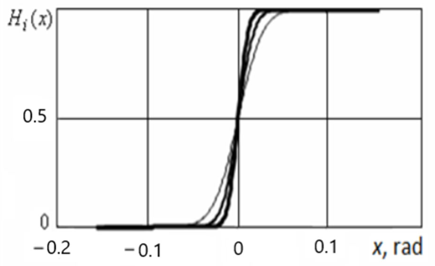
To determine the height of the approximation peak, we use the fact that the δ-function is the derivative of the Heaviside function, or the unit jump function, which is defined as

$$H\left(x\right)=\left\{\begin{array}{c}1, \forall x>0;\\ 0, \forall x<0.\end{array}\right.$$

The Heaviside function can be approximated by a sequence of functions of the form $H_n\left(x\right)=0.5\left(1+f_n\left(x\right)\right)$, where the sequence of functions $f_n\left(x\right)$ is defined by relation (2) and is considered on the interval $[-\pi /2,\pi /2]$.

For example, Figure 18 shows graphs of three successive approximations

$$\begin{gathered} H_9(x)=0.5(1+\sin (A(A(A(A(A(A(A(A(x)))))))))), \\ {H}_{10}(x)=0.5(1+\sin (A(A(A(A(A(A(A(A(A(x)))))))))), \\ {H}_{11}(x)=0.5(1+\sin (A(A(A(A(A(A(A(A(A(A(x))))))))))), \end{gathered}$$

where $A(x)=\frac{\pi }{2}\sin x$.

The thickness of the graph in Figure 18 increases as the number of the approximating dependence increases.

Finding the first derivatives of the approximations of the Heaviside function, we obtain successive approximations $\frac{d{H}_9(x)}{dx}$, $\frac{d{H}_{10}(x)}{dx}$ and $\frac{d{H}_{11}(x)}{dx}$ for the delta function. Their graphs are shown in Figure 19.

With a sufficiently large number of nested functions, we obtain an approximating function $\frac{d{H}_{18}(x)}{dx}$, the graph of which was obtained using the MathCAD computer program and is shown in Figure 17.

Differentiating the approximating functions of the considered sequence $H_n(x)=0.5(1+f_n(x))$, we obtain

$$\frac{d{H}_n(x)}{dx}=\frac{{\pi }^{n-1}}{2^n}{\displaystyle \prod _{k=1}^{n-1}\cos \left(\frac{\pi }{2}{f}_k(x)\right)}\cdot \cos x.$$

Substituting into the resulting expression for the derivatives $x=0$, taking into account the parity of the $\delta$-function, we find the value for the peak height $A_n$ of the approximating functions $H_n(x)$

$$A_n=\frac{{\pi }^{n-1}}{2^n}$$

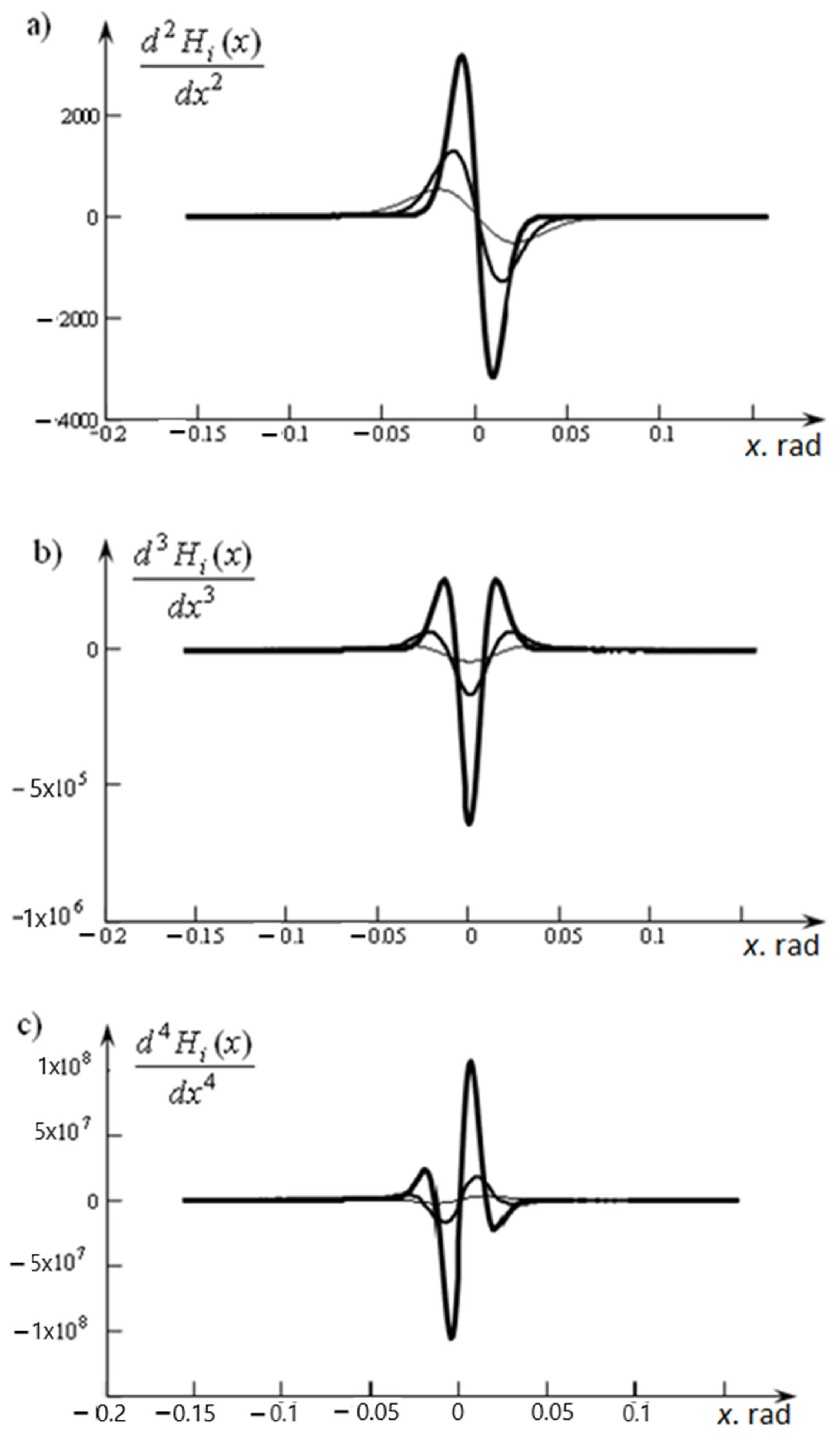
3.5. Approximation of Derivatives of Generalized Functions: Comparison of Approximation Methods

Since we approximated the generalized functions with analytical functions, we can differentiate these approximating functions and find them to obtain approximations of the derivatives of the generalized functions with any degree of accuracy. For example, similarly to how it was conducted in the previous section, we can build graphs of approximations of the derivatives of the δ-function. Figure 20 shows graphs of successive approximations of the first, second and third derivatives of the δ-function.

Derivatives of higher orders can be found in the same way. The plotted graphs give a good idea of the behavior of the derivatives of the δ-function. By mentally increasing the number of the approximating function [11], according to the graphs (Figure 20), it is possible to continue the traced tendencies of changes in the approximations and to present the limiting positions of the sequences of functions approximating the derivatives of the δ-function. This will help to improve the understanding of generalized functions that are derivatives of the δ-function, to use them not just as an abstract mathematical apparatus, but to consciously understand their structure, even if they are written in limiting form. This approach can also be used to better understand other generic functions and their behavior.

The δ-function can also be approximated by other continuously differentiable functions, for example, such

$$\begin{gathered} \delta (x,\alpha )=\frac{\alpha }{\pi ({\alpha }^2{x}^2+1)}, \alpha \to \infty , \\ \delta (x,\alpha )=\frac{\alpha }{\sqrt{\pi }}\exp (-{\alpha }^2{x}^2), \alpha \to \infty , \\ \delta (x,\alpha )=\frac{\alpha }{\pi }\cdot \frac{\sin (\alpha x)}{\alpha x}, \alpha \to \infty , \end{gathered}$$

for which $\underset{\alpha \to \infty }{\lim }\delta (x, \alpha )=0(x\ne 0)$ and $\underset{\alpha \to \infty }{\lim }{\displaystyle \underset{-\infty }{\overset{+\infty }{\int }}\delta (x, \alpha )dx=1}$.

The disadvantage of approximating the δ-function using the third of these functions is a big deviation from the δ-function since this function has not only positive, but also negative values. The graphs of such a function correspond to the graph shown in Figure 10. Moreover, the sequence of negative values is not limited from below, that is, the error can be arbitrarily large.

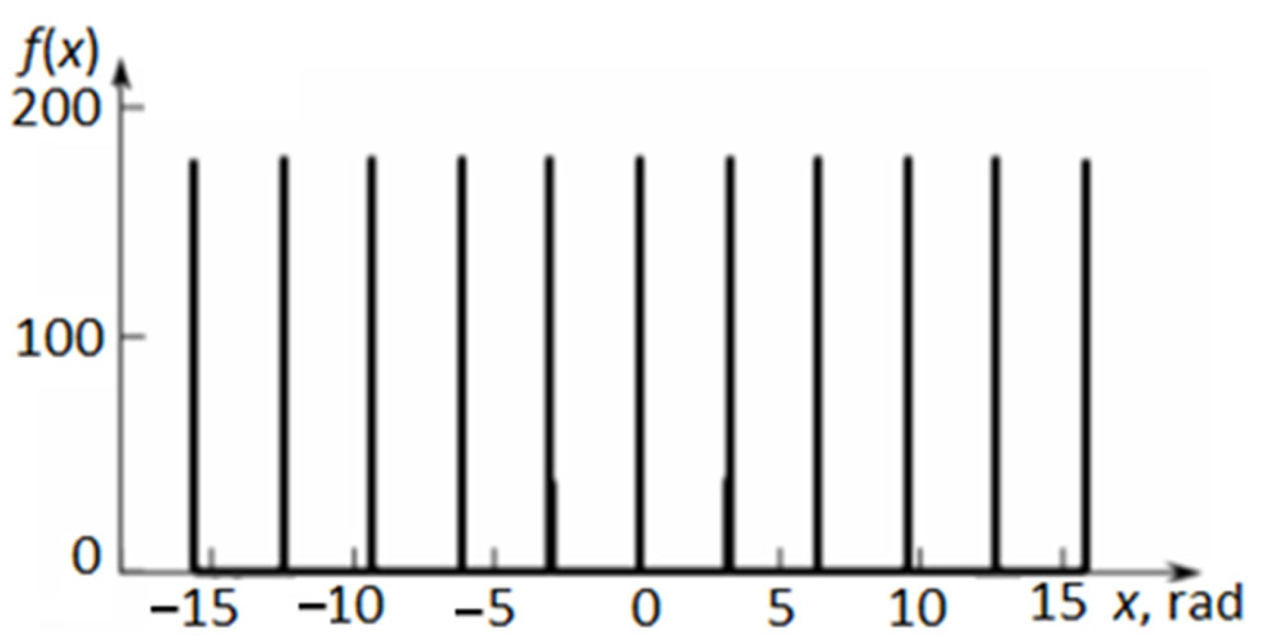
As for the approximation using the first two functions, they allow for approximating the periodic delta function only as a sum $\delta (x)={\displaystyle \sum _{-\infty }^{+\infty }\delta (x-2\pi k)}$, which can be inconvenient for practical use, while the approximating functions according to the proposed method are periodic in nature and allow approximating the periodic delta function without any additional constructions. By a periodic delta function, we mean a generalized function whose argument values, in which the function is not equal to zero, repeat periodically.

An example is the graph of the function

$$f\left(x\right)=\frac{{\pi }^{13}}{2^{14}}\cos (A(A(A(A(A(A(A(A(A(A(A(A(A\left(x\right))))))))))))))),$$

where $A\left(x\right)=\frac{\pi }{2}\sin \left(x\right)$, is shown in Figure 21.

The constructed function $f\left(x\right)$ can be used to approximate the distribution function of a discrete random variable using the relation $F\left(x\right)=P{\int }_{t_0}^{t}f\left(x\right)dx$, where $P$ is a parameter determined from the properties of the distribution function. An example of a distribution function constructed in this way is shown in Figure 22 [5,6,14].

These techniques can be used in the context of mathematical models represented by ODEs or PDEs. For example, in the case of systems with a variable structure, mathematical models are often presented in the form of several systems of differential equations in sections. In this case, problems arise in constructing a solution to equations during a cycle, periodic solutions, the need to track the transitions of the system from section to section and coordinate solutions at the boundaries of sections. Similar problems arise when solving differential equations with piecewise linear and impulse characteristics. The use of the developed approximation methods makes it possible to overcome these problems. In particular, the authors applied the developed methods in studies, the results of which are published in the following articles [6,7,8,9,13,68,69,70] and others.

4. Practical Application and Examples of Using the Developed Approximation Methods

This section of the review discusses various possibilities of using the developed methods for approximating piecewise linear and generalized functions. The examples given are characterized by specific content, a more complete reflection of physical reality. In reality, even fast-flowing processes occur, albeit in a short, but not zero time. For example, in reality there cannot be an instantaneous change in the speed of a material object with a non-zero mass, since such an instantaneous change would require an infinite amount of energy.

4.1. Application of New Methods of Approximation in Problems of Structural Mechanics

The proposed approximation methods, similarly to the Fourier series, are universal. They can be applied in a wide variety of fields of science and technology. One of the many possible examples of the use of these methods in practice is their application in problems of resistance of materials in the broad sense of this term and in problems of structural mechanics in particular.

When calculating building structures such as trusses, beams, etc. it is necessary to take into account the action of distributed and concentrated loads [71]. Loads, as a rule, have piecewise linear characteristics and Fourier series are widely used for their approximation.

Consider, for example, a beam on which a uniformly distributed load with an intensity p acts on a section of length 2c (Figure 23). Other parameters are directly given in Figure 23.

By transforming the argument, without losing the generality of reasoning, we can always consider the load function $f=f\left(x\right)$ only on the interval $\left[-\pi ,\pi \right]$. In this case, the expansion of the load in a Fourier series in our case has the form

$$f\left(x\right)=\frac{pc}{\pi }+\frac{2p}{\pi }{\displaystyle \sum }_{k=1}^{\infty }\frac{1}{k}\sin \left(kc\right)·\cos \left(k\left(x-d\right)\right).$$

Figure 24 shows some other types of loads and their representations in the form of Fourier series.

Similarly, if necessary, you can write down the corresponding Fourier series for other symmetric and asymmetric types of loading of building structures.

The decomposition of loads (acting forces) in Fourier series will have all the disadvantages noted in Section 2.1. Therefore, to eliminate these disadvantages, one can use the proposed approximation methods.

For the load shown in Figure 24a, for $c=\pi /6, d=\pi /2, p=4$ the Fourier series expansion will have the form

$$f\left(x\right)=\frac{4}{3}+\frac{\pi }{16}{\displaystyle \sum }_{k=1}^{\infty }\sin \left(k\frac{\pi }{6}\right)\cos \left(k\frac{\pi }{6}\right)\cos \left(kx\right).$$

Approximating function by the proposed method is found by the expression

$$f\left(x\right)=2-2\sin \left(\frac{\pi }{2}\sin \left(\frac{\pi }{2}\sin \left(\dots \sin \left(0.5+\cos 2x\right)\right)\right)\right).$$

Figure 25 shows the graphs of the original function and its approximating functions. Here, the graph of the original function is highlighted with a thickened stepped line. The graph of the approximating function, constructed using the Fourier series for k = 1, 2, …, 17, is shown by a thin line. The dotted line corresponds to the graph of the approximating function constructed by the proposed method for four nestings.

From Figure 25 we see that, despite the fact that for the expansion in the Fourier series we used seventeen harmonic terms (k = 17), and in the approximation by the proposed method we used only four compositions, the last approximating function approximates the original function much better. Moreover, one could graphically show that a further, arbitrarily large increase in the number of harmonic terms in the Fourier series does not save the situation. The reason for this lies in the aforementioned Gibbs effect.

The advantages of approximating the load using the proposed methods are clearly manifested for concentrated actions on a beam. For example, for the case shown in Figure 26 under the action of two equal in magnitude, but oppositely directed forces applied at symmetrically located points, the expansion in a Fourier series has the form

$$f\left(x\right)=\frac{2P}{\pi }{\sum }_{k=1}^{\infty }\sin \left(kd\right)·\sin \left(kx\right).$$

For $d=\pi /2, P=10$ we approximate this loading scheme by the finite sum of the Fourier series $f\left(x\right)=\frac{2P}{\pi }{\sum }_{k=1}^{20}\sin \left(kd\right)·\sin \left(kx\right)$ and function

$$y\left(x\right)=\cos \left(\frac{\pi }{2}\sin \left(\frac{\pi }{2}\sin \left(\frac{\pi }{2}\sin \left(\frac{\pi }{2}\sin \left(\frac{\pi }{2}\sin \left(\frac{\pi }{2}\cos \left(x\right)\right)\right)\right)\right)\right)\right)·40x.$$

Figure 27 shows the graphs of the obtained approximating functions. The thin line corresponds to the approximation using the Fourier series, the thickened line corresponds to the approximation by the proposed method. As you can see, the results of the approximation clearly speak in favor of the proposed method. We have proposed an approach that allows us to model the load using an analytical function that allows finding derivatives of any order. This function is a single analytical expression for the entire domain of definition and is not composite across sections. This approach can describe a given design load circuit with any degree of accuracy.

4.2. Application of New Approximation Methods for Modeling Diffusion Processes in Semiconductor Materials

Based on the developed methods for approximating piecewise linear and generalized functions, modified models of diffusion processes in semiconductor materials were created [70,72,73,74,75,76]. These models make it possible to provide a more accurate description of diffusion processes in comparison with the known models.

In the modified models, the possibilities of using a new method of continuous approximation of step functions based on the use of trigonometric expressions in the form of recursive functions are considered. Calculations are performed for the classical model of diffusion of minority charge carriers generated by a wide electron beam in a two-layer semiconductor material.

To quantitatively describe the phenomenon of diffusion of nonequilibrium minority charge carriers generated in a semiconductor by an external energy action, the following two approaches are usually used:

(1)

a model of collective motion of minority charge carriers [77,78], according to which diffusion of nonequilibrium minority charge carriers from any microvolume of a semiconductor is influenced by other electrons or holes from other microregions of the material. Mathematically, this is expressed in the fact that the differential diffusion equation as a function of generation of minority charge carriers (usually written in the right-hand side of the differential equation) includes a function that describes the dependence on the coordinates of the density of minority charge carriers generated per unit time in the target. This model is successfully used to quantitatively describe the diffusion processes of minority charge carriers generated by a wide electron beam in homogeneous semiconductors, for which the right-hand side of the differential equation is a continuous function of coordinates. The use of a wide electron beam makes it possible to neglect the edge effects and to solve the one-dimensional problem of heat and mass transfer;

(2)

the model of independent sources, according to which the diffusion of nonequilibrium minority charge carriers from any microvolume of the semiconductor is not influenced by other electrons or holes from other microregions of the material. Mathematically, this is expressed in the fact that first the diffusion equation is solved for each of the point sources of minority charge carriers, after which, by integrating over the volume occupied by the sources of minority charge carriers, their concentration in the semiconductor is found as a result of their diffusion. The idea of this approach is borrowed from classical work [79]. This model was previously used to quantitatively describe the processes of one-dimensional diffusion of minority charge carriers generated by a wide electron beam in inhomogeneous and multilayer planar structures, for which the distribution of electrophysical parameters of materials over depth has break points of the first kind [80,81].

A modification of the first model was proposed, allowing it to be used to simulate the diffusion of minority charge carriers in a two-layer material. The possibility of using this model to solve such a problem appears if, instead of piecewise constant coefficients (electrophysical parameters) of the differential equation of diffusion of minority charge carriers we use their new approximations based on trigonometric expressions in the form of recursive functions [5]. Note that the approximating functions are continuous and analytical, and therefore, at the boundary of the layers, they correspond to a greater extent than step functions to the dependence of the values of real electrophysical parameters on the coordinate [82].

Within the framework of the considered mathematical model, in the case of one-dimensional diffusion into the final semiconductor, the concentration of minority charge carriers in depth is found as a solution to the differential equation [68,70]

$$D\left(z\right)\frac{d^2\Delta p\left(z\right)}{d{z}^2}-\frac{\Delta p\left(z\right)}{\tau \left(z\right)}=-\rho \left(z\right)$$

with boundary conditions

$$D_1\frac{d\Delta p\left(z\right)}{dz}{|}_{z=0}={\nu }_{s_1}\Delta p\left(0\right),\Delta p\left(l\right)=0.$$

In the modified models in the equation, instead of piecewise-constant coefficients (electrophysical parameters), their new approximations are used, based on the use of trigonometric expressions in the form of recursive functions [5]:

$$\begin{array}{c}\left\{f_n\left(z\right)\right|f_n\left(z\right)=\left(\frac{H}{2}\right)\left(1+\sin \left({\phi }_n\left(z\right)\right)\right), {\phi }_n\left(z\right)=\left(\frac{\pi }{2}\right)\sin \left({\phi }_{n-1}\left(z\right)\right),\\ {\phi }_1\left(z\right)=\left(\frac{\pi }{2}\right)f_1\left(z\right), n-1\in N\}.\end{array}$$

As an initial function, a function of the form is taken

$$f_1\left(z\right)=\exp \left(1-{\left(az+b\right)}^2\right)-1.$$

Figure 28 shows the results of calculations carried out using the mathematical package Matlab (MathWorks, Inc., Natick, MA, USA) for the parameters characteristic of the semiconductor structure “epitaxial GaAs film—single-crystal GaAs substrate”.

The following estimates were obtained for the relative error between the exact analytical solution of the problem and the numerical one for n = 5:

$$\Delta =\frac{\underset{0\le i\le n}{\max }\left|\delta p\left(z_i\right)-\delta p_i\right|}{\underset{0\le i\le n}{\max }\left|\delta p\left(z_i\right)\right|}·100\%=9.66\%$$

and for n = 11: $\Delta =0.37\%$.

Thus, for n = 5, the influence of the approximations on the simulation result is visible, and for n = 11, the error in the results is rather small, which indicates the convergence of the approximating procedure used.

The authors of the modified model note [68,70] that the described model allows, with a relatively small number of recursive functions (up to 11), to estimate the concentration of minority charge carriers generated by a wide electron beam in a semiconductor target with an accuracy sufficient for practical use. The model subsequently makes it possible to relatively easily take into account the features of real semiconductor structures (the number and nature of the layers, the space charge region, possibly the energy distribution of electrons that occurs during the interaction of the primary beam with the target, etc.), which makes it promising for quantitative descriptions of the processes of one-dimensional diffusion of minority charge carriers in inhomogeneous and multilayer planar structures.

Note that modified models have been developed for various other examples describing diffusion processes in semiconductor technology [69,70,72,73,74,75,76].

5. Conclusions

As the review has shown, the developed methods for approximating periodic and non-periodic piecewise-linear and generalized functions are undoubtedly promising and have a number of advantages. These methods are characterized by fast convergence and low approximation errors. Similarly to the Fourier series, these methods can be based on the use of well-studied trigonometric functions that have good implementation in applied computer programs. While retaining the positive qualities of the Fourier series in this respect, the new methods are devoid of their drawbacks and can be widely used in solving applied problems. The developed methods are characterized by the complete absence of negative consequences of the Gibbs effect. There is also no wavelike character of the approximation on straight sections of the original piecewise-linear function, even with a small number of nested functions used for approximation.

The proved theorems and properties concerning the convergence and error of the developed approximation methods have confirmed all of the positive aspects of these methods.

The developed methods are illustrated by a large number of theoretical and practical examples taken from a wide variety of areas, so we can confidently speak about the universality of these methods. Despite the wide variety of examples given, these examples by no means exhaust all possible areas of application of new methods. The developed methods can find wide application in the field of signal transmission, the theory of automatic control and regulation systems, mathematical models of technical systems of variable structure, systems with discontinuous characteristics, systems with distributed and concentrated loads and influences, the theory of quantum and mathematical physics, and many other areas. These methods make it possible to find analytical functions for approximating singular generalized functions, and therefore, using differential calculus methods, construct approximations for the derivatives of generalized functions, thereby helping to achieve a better understanding of the meaning of generalized functions when applied to real applied problems. In other words, the developed methods also perform an epistemological function.

Numerical tests carried out on the basis of various practical applications have convincingly shown the correctness of the theoretical studies and the assumptions made.

Note also that the proposed approximating functions are continuous and analytical and even more than step functions correspond to real processes, since in reality even jump-like processes occur, albeit for short, but not zero time intervals. So, for example, an instantaneous change in the speed of a material object requires infinite energy, which is impossible to implement in practice. Concentrated impact in reality does not occur at a point, but is a distributed impact in some small neighborhoods of this point. These realities are fully consistent with the approximating functions obtained using the considered methods based on recursive sequences. In addition, we note that the widespread approximating functions based on splines, for example, are not analytical. Smoothing abrupt changes in the function, the proposed approximation methods bring mathematical models closer to reality, contributing to a deeper understanding of the laws of the world around us.