
Reinforcement Learning-Based Routing Protocols in Flying Ad Hoc Networks (FANET): A Review

 , , and
Abstract
:1. Introduction
- This paper proposes a detailed classification of reinforcement learning-based routing methods in FANETs. This classification includes three main parts: learning algorithm, routing algorithm, and the data dissemination process.
- This paper introduces and compares the state-of-the-art RL-based routing methods in FANETs according to the suggested classification. Furthermore, it studies and reviews the most important advantages and disadvantages of each scheme.
- Finally, this paper expresses some challenges and open issues related to RL-based routing methods in FANETs and presents future research directions.
2. Related Works
3. Fundamentals of Reinforcement Learning (RL)
3.1. Reinforcement Learning
- Reward: This component is a function such as a random function, which depends on state and the action selected by the agent. In fact, it indicates the response of the environment with regard to the selected action. After taking the action, the environment changes its state and produces a reward. The purpose of the agent is to increase the sum of rewards obtained from the interaction with the environment because the reward reflects the main mechanism for modifying the policy. Now, if the agent finds out that the selected action leads to a small reward, it changes its selection and chooses another action when there is a similar condition in the future. This helps the agent to explore different probabilities [19,29].
- Value function: This component is also called the value-action function. Although, the reward represents whether the current selected action is suitable. However, the agent must follow solutions that make more profit in the middle and long term. The value of a certain state represents the sum of received rewards by passing from that state. Thus, actions are selected by searching for the maximum value and not the highest reward. However, it is difficult to calculate the value compared to the reward because the reward is immediately received from the environment. In contrast, the agent must estimate the value by searching for previous interactions with the environment. In all RL algorithms, it is a very challenging issue to estimate the value function [29].
- Model: This component describes the performance of the environment. This model estimates the future state and immediate reward according to a specific state and the selected action. Based on this view, two reinforcement learning methods can be defined: model-based and free-model. Model-based methods design a model for solving RL problems. However, free-model methods learn the optimal policy based on trial and error [18,29].
- Trade-off between exploration and exploitation: Exploration and exploitation are two important concepts in reinforcement learning. In exploration, the agent searches for unknown actions to obtain new knowledge. In exploitation, the agent utilizes the existing knowledge and uses the explored actions to produce high feedback. In the learning process, it is necessary to make a trade-off between exploration and exploitation. The agent can exploit its existing knowledge to achieve the suitable value and can explore new actions to increase its knowledge and obtain more valuable rewards in the future. As a result, the agent should not focus only on exploration or exploitation and must experience various actions to gradually obtain the actions with the highest value.
- Uncertainty: Another challenge for RL is that the agent may face uncertainty when interacting with the environment and updating its state and reward, whereas the purpose of RL is to learn a policy that leads to a high value over time.
3.2. Markov Decision Process
- S indicates the state space.
- A indicates the action space.
- R is the reward function, which is defined as .
- P is defined as the state transition probability .
- γ indicates the discount factor, where .
3.3. Reinforcement Learning Techniques
- Dynamic programming (DP) assumes that there is a complete model of the environment, such as the Markov decision process (MDP). DP consists of a set of solutions that are used to compute the optimal policy according to this model.
- Monte Carlo (MC) approaches are known as the free-model RL techniques, meaning that they do not need to know all the features of an environment. These approaches interact with the environment to achieve experiences. MC methods solve the reinforcement learning problem by averaging sample returns. They are episodic. As a result, MC assumes that the experience is divided into episodes. At the end step, all episodes will be finished no matter what action is selected. Note that the agent can only change values and policies at the end of an episode. Therefore, MC is an incremental episode-by-episode method.
- Q-learning is one of the most important RL algorithms. In this algorithm, the agent tries to learn its optimal actions and store all the state-action pairs and their corresponding values in a Q-table. This table includes two inputs, state and action, and one output called Q-value. In Q-learning, the purpose is to maximize the Q-value.
- State–action–reward–state–action (SARSA), similar to Q-learning, tries to learn MDP. However, SARSA, dissimilar to Q-learning, is an on-policy RL technique that chooses its actions by following the existing policy and changing Q-values in a Q-table. In contrast, an off-policy RL method such as Q-learning does not pursue this policy and selects its actions using a greedy method to maximize the Q-values.
- Deep reinforcement learning (DRL) uses deep learning to improve reinforcement learning and solve complex and difficult issues. Deep learning helps RL agents to become more intelligent, and improves their ability to optimize policies. Compared to other machine learning techniques, RL does not need any dataset. In DRL, the agent interacts with the environment to produce its dataset. Next, DRL uses this dataset to train a deep network.
4. Flying Ad Hoc Networks
- Connectivity: In this network, UAVs have high mobility and low density, which cause the failure of communications between UAVs and affect network connectivity. These features lead to unstable links and high delay in the data transmission process [38].
- Battery: The biggest challenge in these networks is energy consumption because small UAVs use small batteries to supply their required energy for real-time data processing, communications, and flight [38].
- Computational and storage capacity: Flying nodes have limited resources in terms of storage and processing power. It is another challenge in FANETs that must be considered when designing a suitable protocol for sending data packets by UAVs to the ground station [38].
- Delay: Multi-hop communications are suitable for ad hoc networks such as FANETs, which are free-infrastructure, to guarantee end-to-end connectivity. However, this increases delay in the data transmission process. As a result, providing real-time services on these networks is a serious challenge [38].
- Interference management: UAVs are connected to each other through wireless communication. Due to the limited bandwidth capacity in this communication model and dynamic topology in FANETs, interference management is difficult and complex [38].
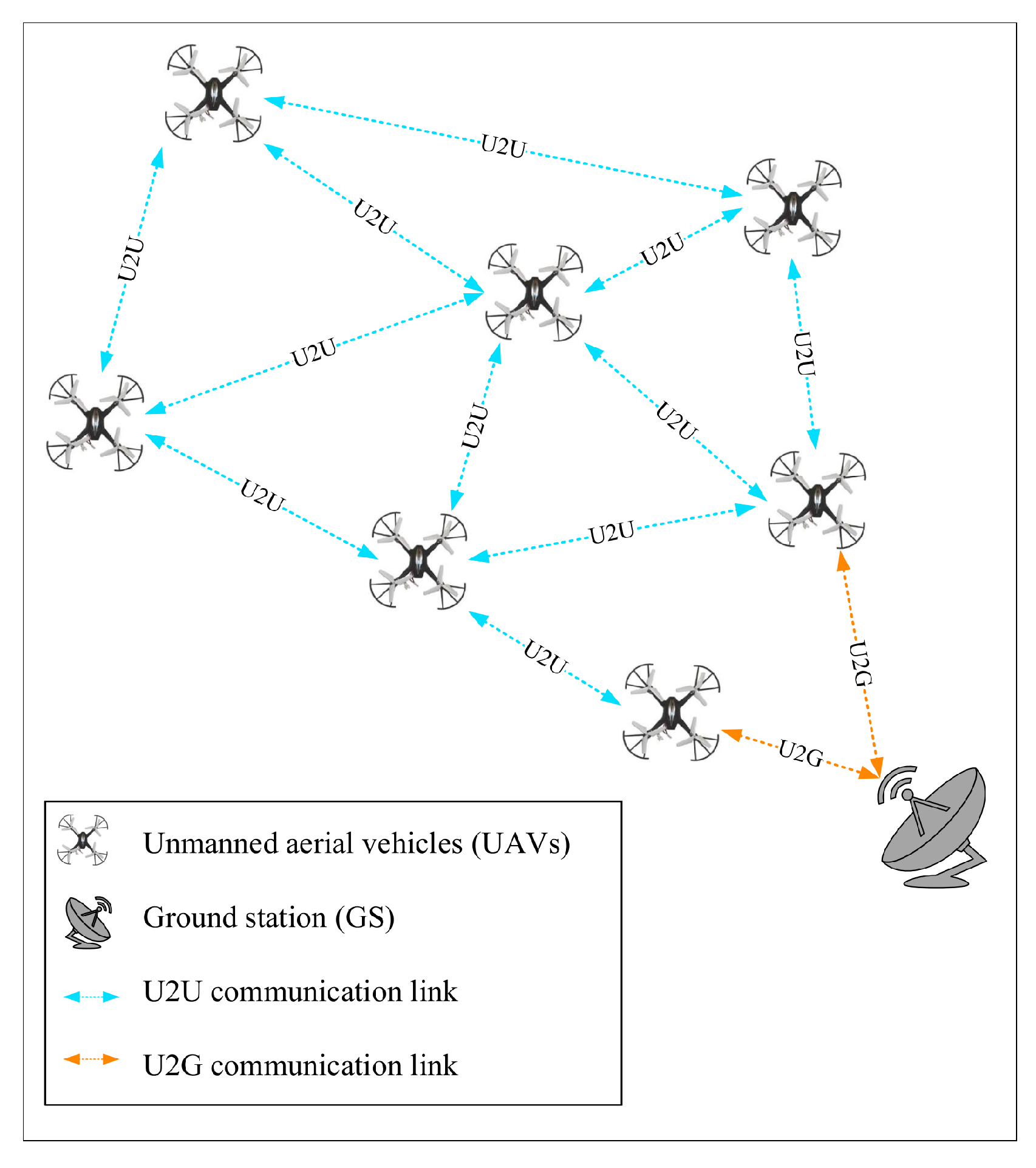
- UAV-to-UAV communication (U2U): As shown in Figure 2, UAVs communicate with each other using U2U communication in a multi-hop manner. This improves their communication range and increases the data rate. This communication is used when a UAV wants to send its data packet to another UAV or ground station beyond its communication radius [39].
- UAV-to-GS communication GS (U2G): As shown in Figure 2, UAVs communicate directly with GS through U2G communication when it is in their communication range. In this communication, GS provides the necessary services to flying nodes, and UAVs send important data to the ground station.
- Hybrid communication: This is a combination of U2U and U2G communications and helps UAVs to send their data to GS in a single-hop or multi-hop manner using intermediate nodes [39].
4.1. Unmanned Aerial Vehicles (UAVs)
- Rotary-wing UAVs (RW-UAVs): These drones can be fixed in the air and perform vertical take-off and landing. As a result, they are more stable and more suitable for indoor areas. However, these drones have higher energy restrictions, slower speeds, and a low capacity compared to fixed-wing UAVs. These features affect their flight time because this time depends on various factors such as path plan, speed, weight, and energy source. RW-UAV is represented in Figure 4a [44,45].
- Fixed-wing UAVs (FW-UAVs): These drones have a longer flight duration, higher flight speed, and aerodynamic design compared to rotary-wing UAVs. These drones can be used for aerial surveillance. They include one body and two wings and are made in different sizes (small and large). However, their weight is more than rotary-wing UAVs. They are similar to traditional aircraft, and cannot be fixed in the air. Therefore, these drones are not suitable for fixed applications. FW-UAVs are displayed in Figure 4b [44,45].
- Remote control-based UAV: These drones are piloted directly by a pilot in line of sight (LoS) or based on feedback received from UAV sensors [45].
- Fully automatic UAV: They perform the flight operations completely independently and without human intervention and can complete their mission when faced with unforeseen operational and environmental conditions [45].
- Low-altitude UAVs: These drones are almost small, lightweight, and cheap. One feature of these drones is that they can easily deploy in an area and fly at a low flight altitude (from 10 meters to a few kilometers). Their speed is very high. However, they suffer from energy restrictions, and therefore, have a short flight duration. Due to fast and easy deployment, these drones are suitable for time-sensitive applications and can be used as an aerial station to provide a high data rate and wireless services at high-risk areas, sports events, and festivals [46].
- High-altitude UAVs: These drones are almost heavy and large and perform their flight operations at a high altitude (more than 10 km). Compared to low-altitude drones, high-altitude UAVs have a longer flight duration and can cover a wide area. However, they are more expensive than low-altitude drones and their deployment is more difficult. They are suitable for applications, which need a longer flight duration and more area coverage. For example, internet broadcasting, remote sensing, and navigation [46].
- Large UAVs: These drones are commonly used in single-UAV systems to carry out some specific missions. They are expensive. Furthermore, their maintenance and repair costs are very high because their structure is complex.
- Small UAVs: These drones can be used in multi-UAV systems and swarms, and are very useful for civilian applications because they have many advantages, including suitable price and less maintenance and repair costs compared to large UAVs. Furthermore, they have simpler structures and include lightweight equipment, such as a cheap body, small batteries, lightweight radio module, and microprocessor. However, their ability is less than larger UAVs. These drones have a short flight time and low coverage range because they are limited in terms of weight and payload. These restrictions can be a serious issue in important missions, for example, search and rescue scenarios.
4.2. Applications
- Search and rescue operations: In this application, flying ad hoc networks can act as the first defensive line during natural disasters due to their fast and easy deployment capability. Furthermore, drones play the role of human relief forces in high-risk areas and pursue specific goals such as finding the precise location of survivors or victims.
- Wildfire monitoring: Flying ad hoc networks can be used to monitor temperature, diagnosis, and prevent fire in forests.
- Traffic monitoring: Highway traffic monitoring is one of the FANET applications. Drones can easily perform this monitoring task to detect gridlock and report traffic management data. This is a viable and economical option. Moreover, these networks can achieve different real-time security solutions to provide security on roads and trains [43].
- Reconnaissance: In aerial surveillance applications, drones fly statically to identify a particular area without human intervention. During surveillance operations, drones collect images of the desired goals and sites in a wide area. This information is quickly processed and sent to a smart control station. When drones oversee a particular target or area, they periodically patrol the target to inspect and monitor their security goals. For example, the border police can identify illegal border crossing through a flying ad hoc network [43].
- Agricultural monitoring: This application is known as precision agriculture. It includes all information technology-based solutions and methods that monitor the health of agricultural products. This application can be upgraded by FANETs to overcome the existing problems in this area. In this case, drones collect information on the quality of agricultural products, growth, and chemical fertilizers in a short period of time and analyze them based on precision scales and criteria [42].
- Remote sensing: Recently, flying ad hoc networks are used with other networks such as wireless sensor networks (WSN). It includes the use of drones equipped with sensors and other equipment. These drones automatically fly throughout the area to obtain information about the desired environment.
- Relaying networks: In this application, drones act as aerial relays to send information collected by ground nodes to base stations efficiently and securely; for example, sending data produced by ground nodes in wireless sensor networks and vehicular ad hoc networks. UAVs are also used to increase the communication range of ground relay nodes.
4.3. Routing
- Limited resources: One of the main challenges in small-sized drones is resource restrictions, including energy, processing power, storage capacity, communication radius, and bandwidth. These restrictions affect the routing protocols. For example, a small communication radius proves that routing protocols should be designed in a multi-hop manner to send data packets to the destination node by assisting intermediate nodes. Limited storage capacity and processing power also indicate that the routing protocol should be optimal and lightweight. Additionally, limited storage capacity and bandwidth can affect the size of packets exchanged on the network. Constrained energy also states that intermediate relay nodes should be carefully selected [13].
- Dynamic topology: FANETs have a highly dynamic topology, which is rooted in the failure of drones due to hardware malfunction, battery discharge, environmental conditions, and the mobility of UAVs. Thus, wireless links between flying nodes must be constantly re-configured. As a result, the routing protocols should be sufficiently flexible to adapt to the dynamic network topology [47].
- Scalability: Flying ad hoc networks have various sizes. This means that they are different in terms of the number of nodes and covered geographical area. Therefore, scalability should be considered when selecting relay nodes (next-hop nodes) on the routing path [13].
- Partitioning and void areas: Another important challenge is that the routing process may be faced with network partitioning and void areas in the network because the FANET is a low-density network. The network partitioning means that one or more network parts cannot connect with other network parts, and the nodes in these parts cannot communicate with the nodes in other network parts. Furthermore, the void area means that one part of the network environment is disconnected, meaning that this area is not covered by flying nodes because there is no node in that part that connects to the outside nodes [47].
- Delay: Delay is the time required to transmit a data packet from the source to destination. When designing a routing algorithm, delay should be considered because real-time applications, such as monitoring, are sensitive to delay. In these applications, a high delay in the data transmission process can lead to unpleasant results [28].
- Packet delivery rate (PDR): It is equal to the ratio of the number of data packets delivered to the destination to the total number of packets sent by the source. Obviously, routing protocols need a higher packet delivery rate. If routing protocols are weakly designed, and the formed paths include routing loops, this has a negative effect on PDR [48].
- Adaptability: This means that routing protocols must quickly react to the network dynamics. For example, if a routing path is broken due to the link failure or discharging battery of nodes, the routing protocol should quickly find the alternative route.
- Load balancing: Routing protocols must evenly distribute their operational load, including energy consumption, calculations, and communications in the network, so that no route does not consume resources faster than other routes [28].
- Routing loops: The routing process should be free-loop to achieve a successful packet delivery rate.
- Routing overhead: Routing protocols must have low routing overhead, meaning that drones can communicate with each other with the least overhead in an efficient routing protocol.
- Communication stability: High mobility of nodes and different environmental conditions such as climate changes can lead to the disconnection of communication links. Therefore, a routing technique must guarantee communication stability in the network.
- Bandwidth: In applications such as aerial imaging, it is very important to consider bandwidth because there are restrictions such as communication channel capacity, drone speed, and sensitivity of wireless links relative to error.
5. Proposed Classification
- Based on the reinforcement learning algorithm;
- Based on the routing algorithm;
- Based on the data dissemination process.
5.1. Classification of RL-Based Routing Protocols Based on Learning Algorithm
5.1.1. Traditional Reinforcement Learning-Based Routing Method
Single-Agent Routing
Multi-Agent Routing
Model-Based Routing
Free-Model Routing
5.1.2. Deep Reinforcement Learning-Based Routing Method
5.2. Classification of RL-Based Routing Protocols Based on Routing Algorithm
- Routing path;
- Network topology;
- Data delivery method;
- Routing process.
5.2.1. Routing Path
- Single-path routing: It means that only one route is formed between the source and destination. Single-path routing is shown in Figure 13. Compared to multi-path routing, this routing method can easily manage routing tables in each UAV. However, single-path routing is not fault-tolerant, meaning that there is no alternative path for sending data packets when failing the routing path. This increases packet loss in the network.
- Multi-path routing: This routing technique creates several routes between the source and destination [55]. Multi-path routing is shown in Figure 14. In this case, it is more difficult to maintain routing tables in UAVs because a UAV may act as intermediate nodes in two or more different paths. This routing method is fault-tolerant, meaning that if one path fails, it is easy to detect and replace this failed path. However, the configuration of this routing scheme is more difficult than the single-path routing approaches because the least errors cause routing loops in the network.
5.2.2. Network Topology
- Hierarchical routing: In this routing technique, UAVs are divided into several hierarchical levels shown in Figure 15. At each level, UAVs can be directly connected to each other. Furthermore, they are connected to a node called the parent node (at their upper level) to communicate with other UAVs at the upper level. The parent node is responsible for managing its children (UAVs at the lower level) and sending their data to the UAVs at the upper level. In this method, determining the different roles for nodes leads to the efficient consumption of the network resources in the route calculation process and reduces routing overhead. This method is scalable. However, there are important research challenges, including the management of different roles and the selection of parent nodes, especially if the UAVs have high mobility in the network. These challenges should be considered in these methods.
- Flat routing: In a flat routing scheme, all UAVs play a similar role in the network, meaning that, dissimilar to hierarchical methods, it does not define any different roles such as parent node and cluster head node in the network to manage the routing process. The flat routing scheme is shown in Figure 16. In this approach, each UAV executes a simple routing algorithm and makes its routing decisions based on its status and neighbors on the network. These routing methods suffer from low scalability and high routing overhead.
5.2.3. Data Delivery Method
- Greedy: The purpose of this routing technique is to reduce the number of hops in the created path between the source UAV and destination UAV. The main principle in the greedy method is that the closest UAV to the destination is geographically selected as a next-hop node, and this process continues until the packet reaches the destination. Figure 17 shows this process. The performance of this method is desirable when the network density is high. However, trapping in a local optimum is the most important weakness of this method. In this case, the data transmission process is stopped at the nearest node to the destination because there is no node closer to the destination. As a result, a path recovery technique is used to find an alternative path and guarantee the reliability of this method.
- Store-carry-forward: This routing technique is efficient when the network is periodically connected and the source node fails to find an intermediate node to send its data packets. In this case, the source UAV must carry this data packet until it finds a suitable relay or destination node. This process is presented in Figure 18. According to this figure, the source UAV has no intermediate node around itself to send data packets. Therefore, it carries its data until it meets the destination UAV. This method is beneficial in low-density networks such as FANETs. In addition, this routing method has low routing overhead and is scalable. However, it is not suitable for real-time applications because it increases delay in the data transmission process.
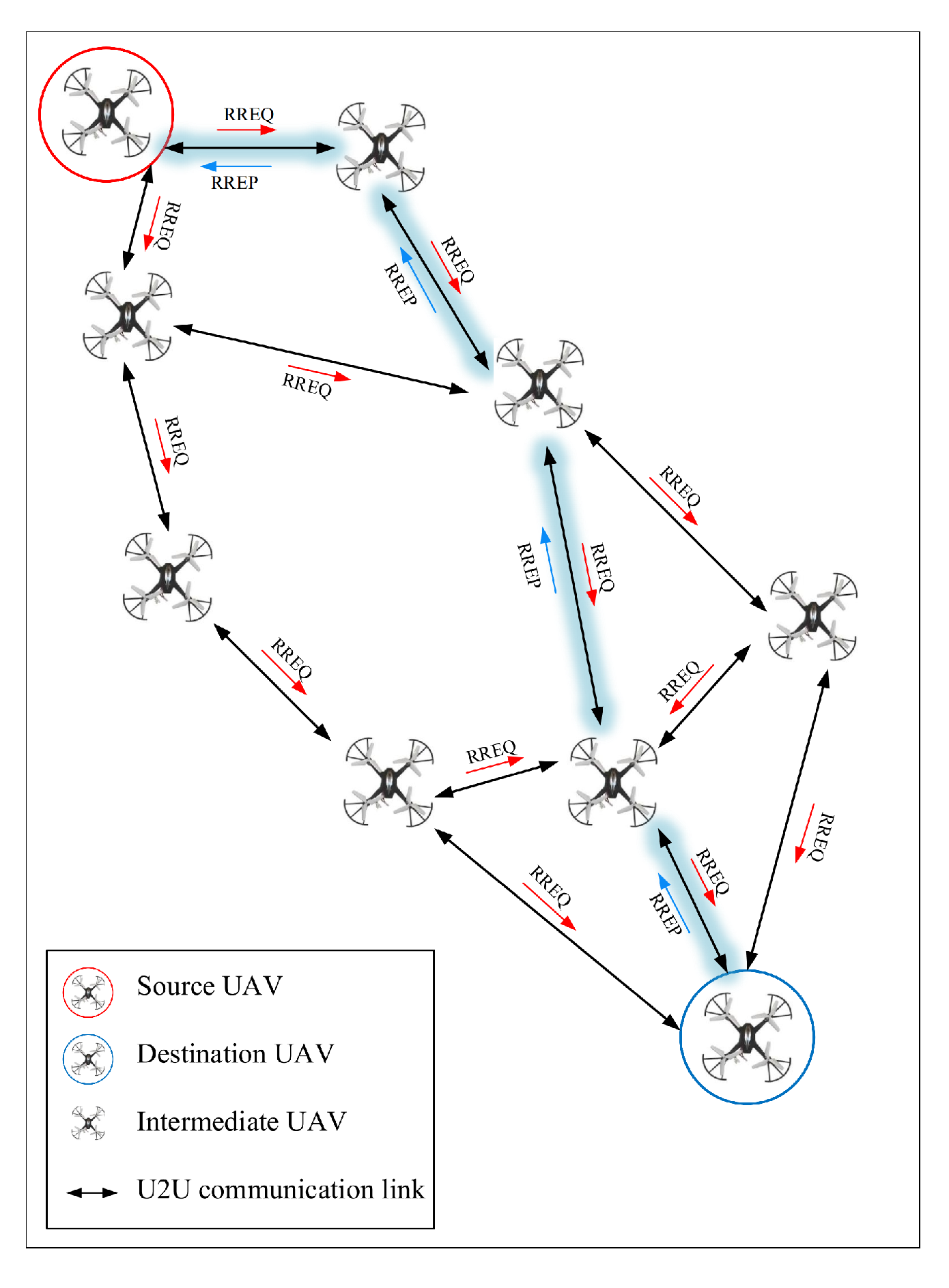
- Route discovery: When the source UAV does not know the geographic position of the destination UAV, the route discovery technique is suitable. In this case, UAVs use the flooding technique and broadcast the route request (RREQ) packets to discover all possible paths to the destination UAV. After receiving the RREQ packet, the destination node is responsible for selecting a suitable path among the discovered paths based on certain criteria. Finally, this route is used to transfer the data packet between source and destination. This process is shown in Figure 19. This routing technique is highly regarded by researchers due to its simplicity. However, it has a high routing overhead due to flooding messages. This issue can lead to a broadcast storm in some cases. This greatly increases bandwidth consumption.
5.2.4. Routing Process
- Centralized routing: In this routing method, a central server manages the routing process. This process is shown in Figure 20. This scheme assumes that the central server has global knowledge of the entire network. The central server is responsible for managing all UAVs and calculating the optimal routing paths on the network. The most important advantage of these methods is that the central server can fully control the entire network and obtains optimal routes at the lowest computational cost. However, this routing technique has disadvantages, such as server maintenance cost, lack of fault-tolerance, single point of failure, high delay, and high routing overhead. In highly dynamic networks such as FANET, it is difficult or even impossible to obtain complete knowledge of the network by the central server. For this reason, these methods are not successful in FANETs, and are not scalable.
- Distributed routing: In this routing method, UAVs share their information with their neighboring UAVs to obtain local knowledge from the network. Then, each UAV participates in the routing process and decides on routing paths based on this limited knowledge. This process is shown in Figure 21. This technique is scalable and flexible because UAVs can quickly and locally react to any issue related to the network dynamics. Therefore, these methods are more suitable for real-time applications. Due to relying on local information, distributed routing methods may form sub-optimal routes and distribute loads using an unbalanced manner in the network. In addition, these methods have more computational overhead compared to centralized routing methods.
5.3. Classification of RL-Based Routing Protocols Based on the Data Dissemination Process
- Unicast-based routing: This routing technique uses point-to-point communication, meaning there is only one source and one destination. In unicast-based routing, UAVs need to know the precise location of themselves and the destination. Thus, they must use a localization system such as a global positioning system (GPS). Figure 22 displays this routing technique. Note that the data traffic in FANETs, similar to other wireless networks, has a broadcast nature. Therefore, a unicast-based routing technique is not compatible with the nature of these networks. These routing methods suffer from problems such as high communication overhead compared to the multicast technique, high delay in the route discovery process, and high bandwidth consumption, and show poor performance in dynamic topology networks [56,57,58].
- Multicast-based routing: Multicast means that data packets are disseminated for a group of UAVs on the network. This method is suitable for applications with limited energy and bandwidth. Multicast-based routing must define multiple multicast groups. A multicast group includes a set of UAVs. Therefore, if a UAV wants to receive a multicast message, it must become a member of a multicast group because when the source UAV sends a multicast message to the multicast group, all group members receive this message. This process is shown in Figure 23. Multicast-based routing protocols use tree-like or mesh-like structures to transfer multicast data from the source to a group of destination nodes. The main weakness of this routing technique is that it must constantly reconstruct the routing tree when changing the network topology [59,60]. This is very challenging in FANETs.
- Broadcast-based routing: In this technique, UAVs flood routing messages in the whole network. This process is represented in Figure 24. The flooding strategy can increase the reception probability of the routing message by the destination, but it consumes a lot of bandwidth. This strategy does not need the spatial information of UAVs in the network and is implemented easily. This method is useful for low-density networks. However, it has a weak performance in dense networks and can cause communication overhead, network congestion, and the broadcast storm problem. The most important disadvantage of this technique is high energy and bandwidth consumption. In addition, this process has a lot of redundancy [61,62,63].
- Geocast-based routing: It is a type of multicast technique. The purpose of this routing technique is to send data packets from the source to all UAVs in a particular geographic area. This process is shown in Figure 25. In this method, the geographic area is inserted into each geocast packet. Then, the geocast packet is delivered to the UAVs in that area. In this method, a geocast group includes a set of nodes in a particular geographic area. To determine the members of this group, each node must know its geographical location on the network. Therefore, they need a positioning system [64,65,66].
6. Investigating Reinforcement Learning-Based Routing Protocols
6.1. DQN-VR
6.2. QTAR
6.3. TQNGPSR
6.4. QMR
6.5. QGeo
6.6. QSRP
6.7. QLGR
6.8. FEQ-Routing-SA
6.9. Q-FANET
6.10. PPMAC+RLSRP
6.11. PARRoT
6.12. QFL-MOR
6.13. 3DQ
6.14. ICRA
- Is the receiver node a CH? If yes, it sends the data packet to the closest CH node or inter-cluster forwarding node to the destination.
- Is the receiver node an inter-cluster forwarding node? If yes, it selects the closest node to the destination among its CH node and its neighboring nodes in other clusters and sends the packet to the selected node.
- Is the receiver node a cluster member node? If yes, it sends this data packet directly to its CH.
6.15. TARRAQ
7. Discussion
8. Challenges and Open Issues
- Mobility models: Most RL-based routing protocols use RWP and GM mobility models to simulate the movement of drones in the network. However, these models cannot simulate the actual movement of drones. Therefore, the simulation results may not guarantee the performance of the routing protocols in real conditions. As a result, in future research directions, researchers must consider realistic mobility models such as [82,83,84,85,86] to simulate the movement of UAVs in the network because they are close to real mobility models and can evaluate the performance of the routing protocols under realistic scenarios.
- Simulation environment: In many RL-based routing protocols, researchers have implemented drones in a two-dimensional environment. However, this implementation is incompatible with the three-dimensional environment of FANETs and affects the performance of these methods. Therefore, researchers must close the simulation environment to the real conditions to evaluate the performance of these protocols more accurately. As a result, deploying the routing methods in a 3D environment and considering all FANET needs and restrictions are subjects that must be studied in future research directions.
- Simulation tool: Most RL-based routing protocols are simulated using simulators such as WSNet, NS3, and MATLAB to evaluate their performance in a virtual environment. They require low cost. However, these tools cannot accurately simulate a real environment, and the simulation results do not usually match the real environment. Therefore, these methods must be implemented in real environments to analyze their performance in real conditions. However, this is extremely expensive.
- Localization: Most RL-based routing methods must obtain location information using a positioning system. Therefore, their performance is dependent on a positioning system. If the positioning system is not accurate and cannot properly measure the position of drones, the network performance will be weakened. GPS is the most common positioning system used in RL-based routing protocols. The accuracy of this positioning system depends on environmental conditions. For example, if UAVs are in an open environment with a good climate, GPS can predict the position of drones with proper accuracy. In contrast, in indoor areas such as tunnels or in inappropriate weather conditions, GPS signals are not properly received. This has a negative effect on network performance. Focusing on free infrastructure localization methods and calculating the position of nodes without the need for GPS is a good solution, which can be considered by researchers in the future.
- Efficiency: Reinforcement learning algorithms are useful for designing RL-based routing methods in FANETs when they can solve a serious problem in this area. These algorithms can improve the routing policy and build an optimal path between nodes in the network, but impose a lot of computational costs on UAVs in the network. When designing a RL-based routing method, researchers must determine whether these algorithms help routing protocols to improve network performance and reduce computational cost and energy consumption. In some cases, solving a challenge in FANETs may not need to use reinforcement learning techniques, and existing methods can successfully address this challenge. As a result, proper use of reinforcement learning techniques is a very important issue, which must be considered by researchers.
- Routing overhead: In most RL-based routing methods in FANETs, the periodic exchange of control messages is essential to obtain the location and other information of neighboring nodes. However, this increases bandwidth consumption and routing overhead and greatly increases network congestion. Therefore, an essential need is to adaptively adjust the broadcast intervals of these messages based on network dynamics when designing RL-based routing methods.
- Convergence speed: It is an important issue in reinforcement learning algorithms. When the size of the state and action spaces are large, the convergence speed of the RL algorithm is greatly reduced. Thus, obtaining an optimal response requires a long time. In this case, the Q-table size also increases sharply. This needs a large storage capacity to store this table. On the other hand, the update process of this table is also associated with high delay, computational costs, and communication overhead. Therefore, reducing the size of the state space by filtering some states based on specific criteria and utilizing clustering techniques in the routing process can be studied and evaluated in the future. Furthermore, the use of deep reinforcement learning techniques is a useful response to deal with this challenge.
- Trade-off between exploration and exploitation: The dynamic adjustment of learning parameters, including learning rate and the discount factor, is very important in a RL-based routing algorithm to create a balance between exploration and exploitation. Researchers should consider this issue in the future.
9. Conclusions
Author Contributions
Funding
Institutional Review Board Statement
Informed Consent Statement
Data Availability Statement
Acknowledgments
Conflicts of Interest
References
- Sharma, V.; Kumar, R. Cooperative frameworks and network models for flying ad hoc networks: A survey. Concurr. Comput. Pract. Exp. 2017, 29, e3931. [Google Scholar] [CrossRef]
- Yousefpoor, M.S.; Barati, H. Dynamic key management algorithms in wireless sensor networks: A survey. Comput. Commun. 2019, 134, 52–69. [Google Scholar] [CrossRef]
- Siddiqi, M.A.; Iwendi, C.; Jaroslava, K.; Anumbe, N. Analysis on security-related concerns of unmanned aerial vehicle: Attacks, limitations, and recommendations. Math. Biosci. Eng. 2022, 19, 2641–2670. [Google Scholar] [CrossRef] [PubMed]
- Yousefpoor, M.S.; Barati, H. DSKMS: A dynamic smart key management system based on fuzzy logic in wireless sensor networks. Wirel. Netw. 2020, 26, 2515–2535. [Google Scholar] [CrossRef]
- Lakew, D.S.; Sa’ad, U.; Dao, N.N.; Na, W.; Cho, S. Routing in flying ad hoc networks: A comprehensive survey. IEEE Commun. Surv. Tutor. 2020, 22, 1071–1120. [Google Scholar] [CrossRef]
- Yousefpoor, M.S.; Yousefpoor, E.; Barati, H.; Barati, A.; Movaghar, A.; Hosseinzadeh, M. Secure data aggregation methods and countermeasures against various attacks in wireless sensor networks: A comprehensive review. J. Netw. Comput. Appl. 2021, 190, 103118. [Google Scholar] [CrossRef]
- Oubbati, O.S.; Atiquzzaman, M.; Lorenz, P.; Tareque, M.H.; Hossain, M.S. Routing in flying ad hoc networks: Survey, constraints, and future challenge perspectives. IEEE Access 2019, 7, 81057–81105. [Google Scholar] [CrossRef]
- Rahmani, A.M.; Ali, S.; Yousefpoor, M.S.; Yousefpoor, E.; Naqvi, R.A.; Siddique, K.; Hosseinzadeh, M. An area coverage scheme based on fuzzy logic and shuffled frog-leaping algorithm (sfla) in heterogeneous wireless sensor networks. Mathematics 2021, 9, 2251. [Google Scholar] [CrossRef]
- Xu, M.; Xie, J.; Xia, Y.; Liu, W.; Luo, R.; Hu, S.; Huang, D. Improving traditional routing protocols for flying ad hoc networks: A survey. In Proceedings of the 2020 IEEE 6th International Conference on Computer and Communications (ICCC), Chengdu, China, 11–14 December 2020; pp. 162–166. [Google Scholar] [CrossRef]
- Lee, S.W.; Ali, S.; Yousefpoor, M.S.; Yousefpoor, E.; Lalbakhsh, P.; Javaheri, D.; Rahmani, A.M.; Hosseinzadeh, M. An energy-aware and predictive fuzzy logic-based routing scheme in flying ad hoc networks (fanets). IEEE Access 2021, 9, 129977–130005. [Google Scholar] [CrossRef]
- Mukherjee, A.; Keshary, V.; Pandya, K.; Dey, N.; Satapathy, S.C. Flying ad hoc networks: A comprehensive survey. Inf. Decis. Sci. 2018, 701, 569–580. [Google Scholar] [CrossRef]
- Rahmani, A.M.; Ali, S.; Yousefpoor, E.; Yousefpoor, M.S.; Javaheri, D.; Lalbakhsh, P.; Ahmed, O.H.; Hosseinzadeh, M.; Lee, S.W. OLSR+: A new routing method based on fuzzy logic in flying ad hoc networks (FANETs). Veh. Commun. 2022, 36, 100489. [Google Scholar] [CrossRef]
- Oubbati, O.S.; Lakas, A.; Zhou, F.; Güneş, M.; Yagoubi, M.B. A survey on position-based routing protocols for Flying Ad hoc Networks (FANETs). Veh. Commun. 2017, 10, 29–56. [Google Scholar] [CrossRef]
- Mohammed, M.; Khan, M.B.; Bashier, E.B.M. Machine Learning: Algorithms and Applications; CRC Press: Boca Raton, FL, USA, 2016. [Google Scholar]
- Rahmani, A.M.; Yousefpoor, E.; Yousefpoor, M.S.; Mehmood, Z.; Haider, A.; Hosseinzadeh, M.; Ali Naqvi, R. Machine learning (ML) in medicine: Review, applications, and challenges. Mathematics 2021, 9, 2970. [Google Scholar] [CrossRef]
- Uprety, A.; Rawat, D.B. Reinforcement learning for iot security: A comprehensive survey. IEEE Internet Things J. 2020, 8, 8693–8706. [Google Scholar] [CrossRef]
- Padakandla, S. A survey of reinforcement learning algorithms for dynamically varying environments. ACM Comput. Surv. (CSUR) 2021, 54, 1–25. [Google Scholar] [CrossRef]
- Wang, Q.; Zhan, Z. Reinforcement learning model, algorithms and its application. In Proceedings of the 2011 International Conference on Mechatronic Science, Electric Engineering and Computer (MEC), Jilin, China, 19–22 August 2011; pp. 1143–1146. [Google Scholar] [CrossRef]
- Al-Rawi, H.A.; Ng, M.A.; Yau, K.L.A. Application of reinforcement learning to routing in distributed wireless networks: A review. Artif. Intell. Rev. 2015, 43, 381–416. [Google Scholar] [CrossRef]
- Rovira-Sugranes, A.; Razi, A.; Afghah, F.; Chakareski, J. A review of AI-enabled routing protocols for UAV networks: Trends, challenges, and future outlook. Ad Hoc Netw. 2022, 130, 102790. [Google Scholar] [CrossRef]
- Rezwan, S.; Choi, W. A survey on applications of reinforcement learning in flying ad hoc networks. Electronics 2021, 10, 449. [Google Scholar] [CrossRef]
- Alam, M.M.; Moh, S. Survey on Q-Learning-Based Position-Aware Routing Protocols in Flying Ad Hoc Networks. Electronics 2022, 11, 1099. [Google Scholar] [CrossRef]
- Bithas, P.S.; Michailidis, E.T.; Nomikos, N.; Vouyioukas, D.; Kanatas, A.G. A survey on machine-learning techniques for UAV-based communications. Sensors 2019, 19, 5170. [Google Scholar] [CrossRef] [Green Version]
- Srivastava, A.; Prakash, J. Future FANET with application and enabling techniques: Anatomization and sustainability issues. Comput. Sci. Rev. 2021, 39, 100359. [Google Scholar] [CrossRef]
- Suthaputchakun, C.; Sun, Z. Routing protocol in intervehicle communication systems: A survey. IEEE Commun. Mag. 2011, 49, 150–156. [Google Scholar] [CrossRef]
- Maxa, J.A.; Mahmoud, M.S.B.; Larrieu, N. Survey on UAANET routing protocols and network security challenges. Adhoc Sens. Wirel. Netw. 2017, 37, 231–320. [Google Scholar]
- Jiang, J.; Han, G. Routing protocols for unmanned aerial vehicles. IEEE Commun. Mag. 2018, 56, 58–63. [Google Scholar] [CrossRef]
- Arafat, M.Y.; Moh, S. Routing protocols for unmanned aerial vehicle networks: A survey. IEEE Access 2019, 7, 99694–99720. [Google Scholar] [CrossRef]
- Coronato, A.; Naeem, M.; De Pietro, G.; Paragliola, G. Reinforcement learning for intelligent healthcare applications: A survey. Artif. Intell. Med. 2020, 109, 101964. [Google Scholar] [CrossRef]
- Kubat, M. An Introduction to Machine Learning; Springer International Publishing: Cham, Switzerland, 2017; Volume 2. [Google Scholar] [CrossRef]
- Rahmani, A.M.; Ali, S.; Malik, M.H.; Yousefpoor, E.; Yousefpoor, M.S.; Mousavi, A.; Hosseinzadeh, M. An energy-aware and Q-learning-based area coverage for oil pipeline monitoring systems using sensors and Internet of Things. Sci. Rep. 2022, 12, 1–17. [Google Scholar] [CrossRef]
- Javaheri, D.; Hosseinzadeh, M.; Rahmani, A.M. Detection and elimination of spyware and ransomware by intercepting kernel-level system routines. IEEE Access 2018, 6, 78321–78332. [Google Scholar] [CrossRef]
- Nazib, R.A.; Moh, S. Routing protocols for unmanned aerial vehicle-aided vehicular ad hoc networks: A survey. IEEE Access 2020, 8, 77535–77560. [Google Scholar] [CrossRef]
- Yousefpoor, E.; Barati, H.; Barati, A. A hierarchical secure data aggregation method using the dragonfly algorithm in wireless sensor networks. Peer-Peer Netw. Appl. 2021, 14, 1917–1942. [Google Scholar] [CrossRef]
- Vijitha Ananthi, J.; Subha Hency Jose, P. A review on various routing protocol designing features for flying ad hoc networks. Mob. Comput. Sustain. Inform. 2022, 68, 315–325. [Google Scholar] [CrossRef]
- Azevedo, M.I.B.; Coutinho, C.; Toda, E.M.; Carvalho, T.C.; Jailton, J. Wireless communications challenges to flying ad hoc networks (FANET). Mob. Comput. 2020, 3. [Google Scholar] [CrossRef] [Green Version]
- Wang, J.; Jiang, C. Flying Ad Hoc Networks: Cooperative Networking and Resource Allocation; Springer: Berlin/Heidelberg, Germany, 2022. [Google Scholar] [CrossRef]
- Noor, F.; Khan, M.A.; Al-Zahrani, A.; Ullah, I.; Al-Dhlan, K.A. A review on communications perspective of flying ad hoc networks: Key enabling wireless technologies, applications, challenges and open research topics. Drones 2020, 4, 65. [Google Scholar] [CrossRef]
- Guillen-Perez, A.; Cano, M.D. Flying ad hoc networks: A new domain for network communications. Sensors 2018, 18, 3571. [Google Scholar] [CrossRef] [PubMed] [Green Version]
- Agrawal, J.; Kapoor, M. A comparative study on geographic-based routing algorithms for flying ad hoc networks. Concurr. Comput. Pract. Exp. 2021, 33, e6253. [Google Scholar] [CrossRef]
- Kim, D.Y.; Lee, J.W. Topology construction for flying ad hoc networks (FANETs). In Proceedings of the 2017 International Conference on Information and Communication Technology Convergence (ICTC), Jeju Island, Korea, 18–20 October 2017; pp. 153–157. [Google Scholar] [CrossRef]
- Rahman, M.F.F.; Fan, S.; Zhang, Y.; Chen, L. A comparative study on application of unmanned aerial vehicle systems in agriculture. Agriculture 2021, 11, 22. [Google Scholar] [CrossRef]
- Shrestha, R.; Bajracharya, R.; Kim, S. 6G enabled unmanned aerial vehicle traffic management: A perspective. IEEE Access 2021, 9, 91119–91136. [Google Scholar] [CrossRef]
- Liu, T.; Sun, Y.; Wang, C.; Zhang, Y.; Qiu, Z.; Gong, W.; Lei, S.; Tong, X.; Duan, X. Unmanned aerial vehicle and artificial intelligence revolutionizing efficient and precision sustainable forest management. J. Clean. Prod. 2021, 311, 127546. [Google Scholar] [CrossRef]
- Idrissi, M.; Salami, M.; Annaz, F. A Review of Quadrotor Unmanned Aerial Vehicles: Applications, Architectural Design and Control Algorithms. J. Intell. Robot. Syst. 2022, 104, 1–33. [Google Scholar] [CrossRef]
- Syed, F.; Gupta, S.K.; Hamood Alsamhi, S.; Rashid, M.; Liu, X. A survey on recent optimal techniques for securing unmanned aerial vehicles applications. Trans. Emerg. Telecommun. Technol. 2021, 32, e4133. [Google Scholar] [CrossRef]
- Sang, Q.; Wu, H.; Xing, L.; Xie, P. Review and comparison of emerging routing protocols in flying ad hoc networks. Symmetry 2020, 12, 971. [Google Scholar] [CrossRef]
- Mittal, M.; Iwendi, C. A survey on energy-aware wireless sensor routing protocols. EAI Endorsed Trans. Energy Web 2019, 6. [Google Scholar] [CrossRef]
- Agostinelli, F.; Hocquet, G.; Singh, S.; Baldi, P. From reinforcement learning to deep reinforcement learning: An overview. In Braverman Readings in Machine Learning. Key Ideas from Inception to Current State; Springer: Berlin/Heidelberg, Germany, 2018; pp. 298–328. [Google Scholar] [CrossRef]
- Althamary, I.; Huang, C.W.; Lin, P. A survey on multi-agent reinforcement learning methods for vehicular networks. In Proceedings of the 2019 15th International Wireless Communications & Mobile Computing Conference (IWCMC), Tangier, Morocco, 24–28 June 2019; pp. 1154–1159. [Google Scholar] [CrossRef]
- Canese, L.; Cardarilli, G.C.; Di Nunzio, L.; Fazzolari, R.; Giardino, D.; Re, M.; Spanò, S. Multi-agent reinforcement learning: A review of challenges and applications. Appl. Sci. 2021, 11, 4948. [Google Scholar] [CrossRef]
- Busoniu, L.; Babuska, R.; De Schutter, B. A comprehensive survey of multiagent reinforcement learning. IEEE Trans. Syst. Man, Cybern. Part C Appl. Rev. 2008, 38, 156–172. [Google Scholar] [CrossRef] [Green Version]
- Drummond, N.; Niv, Y. Model-based decision making and model-free learning. Curr. Biol. 2020, 30, R860–R865. [Google Scholar] [CrossRef] [PubMed]
- Asadi, K. Strengths, Weaknesses, and Combinations of Model-Based and Model-Free Reinforcement Learning. Master’s Thesis, Department of Computing Science, University of Alberta, Edmonton, AB, Canada, 2015. [Google Scholar]
- Sirajuddin, M.; Rupa, C.; Iwendi, C.; Biamba, C. TBSMR: A trust-based secure multipath routing protocol for enhancing the qos of the mobile ad hoc network. Secur. Commun. Netw. 2021, 2021. [Google Scholar] [CrossRef]
- Bernsen, J.; Manivannan, D. Unicast routing protocols for vehicular ad hoc networks: A critical comparison and classification. Pervasive Mob. Comput. 2009, 5, 1–18. [Google Scholar] [CrossRef]
- Panichpapiboon, S.; Pattara-Atikom, W. A review of information dissemination protocols for vehicular ad hoc networks. IEEE Commun. Surv. Tutor. 2011, 14, 784–798. [Google Scholar] [CrossRef]
- Ren, Z.; Guo, W. Unicast routing in mobile ad hoc networks: Present and future directions. In Proceedings of the Fourth International Conference on Parallel and Distributed Computing, Applications and Technologies, Chengdu, China, 29 August 2003; pp. 340–344. [Google Scholar] [CrossRef]
- Biradar, R.C.; Manvi, S.S. Review of multicast routing mechanisms in mobile ad hoc networks. J. Netw. Comput. Appl. 2012, 35, 221–239. [Google Scholar] [CrossRef]
- Guo, S.; Yang, O.W. Energy-aware multicasting in wireless ad hoc networks: A survey and discussion. Comput. Commun. 2007, 30, 2129–2148. [Google Scholar] [CrossRef]
- Khabbazian, M.; Bhargava, V.K. Efficient broadcasting in mobile ad hoc networks. IEEE Trans. Mob. Comput. 2008, 8, 231–245. [Google Scholar] [CrossRef]
- Reina, D.G.; Toral, S.L.; Johnson, P.; Barrero, F. A survey on probabilistic broadcast schemes for wireless ad hoc networks. Ad Hoc Netw. 2015, 25, 263–292. [Google Scholar] [CrossRef] [Green Version]
- Ruiz, P.; Bouvry, P. Survey on broadcast algorithms for mobile ad hoc networks. ACM Comput. Surv. (CSUR) 2015, 48, 1–35. [Google Scholar] [CrossRef]
- Ko, Y.B.; Vaidya, N.H. Flooding-based geocasting protocols for mobile ad hoc networks. Mob. Netw. Appl. 2002, 7, 471–480. [Google Scholar] [CrossRef]
- Drouhin, F.; Bindel, S. Routing and Data Diffusion in Vehicular Ad Hoc Networks. In Building Wireless Sensor Networks; Elsevier: Amsterdam, The Netherlands, 2017; pp. 67–96. [Google Scholar] [CrossRef]
- Mohapatra, P.; Li, J.; Gui, C. Multicasting in ad hoc networks. In Ad Hoc Networks; Springer: Boston, MA, USA, 2005; pp. 91–122. [Google Scholar] [CrossRef]
- Khan, M.F.; Yau, K.L.A.; Ling, M.H.; Imran, M.A.; Chong, Y.W. An Intelligent Cluster-Based Routing Scheme in 5G Flying Ad Hoc Networks. Appl. Sci. 2022, 12, 3665. [Google Scholar] [CrossRef]
- Arafat, M.Y.; Moh, S. A Q-learning-based topology-aware routing protocol for flying ad hoc networks. IEEE Internet Things J. 2021, 9, 1985–2000. [Google Scholar] [CrossRef]
- Chen, Y.N.; Lyu, N.Q.; Song, G.H.; Yang, B.W.; Jiang, X.H. A traffic-aware Q-network enhanced routing protocol based on GPSR for unmanned aerial vehicle ad hoc networks. Front. Inf. Technol. Electron. Eng. 2020, 21, 1308–1320. [Google Scholar] [CrossRef]
- Liu, J.; Wang, Q.; He, C.; Jaffrès-Runser, K.; Xu, Y.; Li, Z.; Xu, Y. QMR: Q-learning based multi-objective optimization routing protocol for flying ad hoc networks. Comput. Commun. 2020, 150, 304–316. [Google Scholar] [CrossRef]
- Jung, W.S.; Yim, J.; Ko, Y.B. QGeo: Q-learning-based geographic ad hoc routing protocol for unmanned robotic networks. IEEE Commun. Lett. 2017, 21, 2258–2261. [Google Scholar] [CrossRef]
- Lim, J.W.; Ko, Y.B. Q-learning based stepwise routing protocol for multi-uav networks. In Proceedings of the 2021 International Conference on Artificial Intelligence in Information and Communication (ICAIIC), Jeju Island, Korea, 13–16 April 2021; pp. 307–309. [Google Scholar] [CrossRef]
- Qiu, X.; Xie, Y.; Wang, Y.; Ye, L.; Yang, Y. QLGR: A Q-learning-based Geographic FANET Routing Algorithm Based on Multi-agent Reinforcement Learning. KSII Trans. Internet Inf. Syst. (TIIS) 2021, 15, 4244–4274. [Google Scholar] [CrossRef]
- Rovira-Sugranes, A.; Afghah, F.; Qu, J.; Razi, A. Fully-echoed q-routing with simulated annealing inference for flying adhoc networks. IEEE Trans. Netw. Sci. Eng. 2021, 8, 2223–2234. [Google Scholar] [CrossRef]
- Da Costa, L.A.L.; Kunst, R.; de Freitas, E.P. Q-FANET: Improved Q-learning based routing protocol for FANETs. Comput. Netw. 2021, 198, 108379. [Google Scholar] [CrossRef]
- Zheng, Z.; Sangaiah, A.K.; Wang, T. Adaptive communication protocols in flying ad hoc network. IEEE Commun. Mag. 2018, 56, 136–142. [Google Scholar] [CrossRef]
- Sliwa, B.; Schüler, C.; Patchou, M.; Wietfeld, C. PARRoT: Predictive ad hoc routing fueled by reinforcement learning and trajectory knowledge. In Proceedings of the 2021 IEEE 93rd Vehicular Technology Conference (VTC2021-Spring), Helsinki, Finland, 25–28 April 2021; pp. 1–7. [Google Scholar] [CrossRef]
- Yang, Q.; Jang, S.J.; Yoo, S.J. Q-learning-based fuzzy logic for multi-objective routing algorithm in flying ad hoc networks. Wirel. Pers. Commun. 2020, 113, 115–138. [Google Scholar] [CrossRef]
- Zhang, M.; Dong, C.; Feng, S.; Guan, X.; Chen, H.; Wu, Q. Adaptive 3D routing protocol for flying ad hoc networks based on prediction-driven Q-learning. China Commun. 2022, 19, 302–317. [Google Scholar] [CrossRef]
- Guo, J.; Gao, H.; Liu, Z.; Huang, F.; Zhang, J.; Li, X.; Ma, J. ICRA: An Intelligent Clustering Routing Approach for UAV Ad Hoc Networks. IEEE Trans. Intell. Transp. Syst. 2022, 1–14. [Google Scholar] [CrossRef]
- Cui, Y.; Zhang, Q.; Feng, Z.; Wei, Z.; Shi, C.; Yang, H. Topology-Aware Resilient Routing Protocol for FANETs: An Adaptive Q-Learning Approach. IEEE Internet Things J. 2022. [Google Scholar] [CrossRef]
- Zhao, H.; Liu, H.; Leung, Y.W.; Chu, X. Self-adaptive collective motion of swarm robots. IEEE Trans. Autom. Sci. Eng. 2018, 15, 1533–1545. [Google Scholar] [CrossRef]
- Xu, W.; Xiang, L.; Zhang, T.; Pan, M.; Han, Z. Cooperative Control of Physical Collision and Transmission Power for UAV Swarm: A Dual-Fields Enabled Approach. IEEE Internet Things J. 2021, 9, 2390–2403. [Google Scholar] [CrossRef]
- Dai, F.; Chen, M.; Wei, X.; Wang, H. Swarm intelligence-inspired autonomous flocking control in UAV networks. IEEE Access 2019, 7, 61786–61796. [Google Scholar] [CrossRef]
- Zhao, H.; Wei, J.; Huang, S.; Zhou, L.; Tang, Q. Regular topology formation based on artificial forces for distributed mobile robotic networks. IEEE Trans. Mob. Comput. 2018, 18, 2415–2429. [Google Scholar] [CrossRef]
- Trotta, A.; Montecchiari, L.; Di Felice, M.; Bononi, L. A GPS-free flocking model for aerial mesh deployments in disaster-recovery scenarios. IEEE Access 2020, 8, 91558–91573. [Google Scholar] [CrossRef]


| Algorithm | Advantage | Disadvantages |
|---|---|---|
| Dynamic programming (DP) | Acceptable convergence speed | Considering a complete model of the environment, high computational complexity |
| Monte Carlo (MC) | A free-model reinforcement learning method | High return variance, low convergence speed, trapping in local optimum |
| Q-learning | A free-model, off-policy, and forward reinforcement learning | Lack of generalization, inability to predict the optimal value for unseen states |
| State–action–reward–state–action (SARSA) | A free-model, on-policy, and forward reinforcement learning | Lack of generalization, inability to predict the optimal value for unseen states |
| Deep reinforcement learning (DRL) | Suitable for solving problems with high dimensions, the ability to estimate unseen states, the ability to generalization | Being unstable model, making rapid changes in the policy with little change in Q-value |
| Routing Scheme | Convergence Speed | Computational Cost | Generalization | Learning Speed | Scalability | State and Action Spaces | Implementation | Fault-Tolerance | |
|---|---|---|---|---|---|---|---|---|---|
| RL-based | Single-agent | Low | Low | No | Low | Low | Small | Simple | No |
| Multi-agent | High | Very high | No | High | Medium | Medium | Complex | Yes | |
| Model-based | High | Very high | No | Low | Low | Small | Complex | No | |
| Free-model | Medium | Low | No | Medium | Medium | Small | Simple | No | |
| DRL-based | Single-agent | High | High | Yes | High | High | Large | Complex | No |
| Multi-agent | Very high | Very high | Yes | Very high | High | Large | Complex | Yes | |
| Model-based | High | Very high | Yes | Medium | High | Large | Complex | No | |
| Free-model | High | High | Yes | High | High | Large | Complex | No | |
| Routing Scheme | Routing Table Management | Packet Loss | Fault-Tolerance | Network Congestion | Routing Loop |
|---|---|---|---|---|---|
| Single-path | Simple | High | No | High | Low |
| Multi-path | Complex | Low | Yes | Low | High |
| Routing Scheme | Management of Node Roles | Scalability | Routing Overhead | Network Congestion | Energy Consumption | Network Lifetime |
|---|---|---|---|---|---|---|
| Hierarchical | Difficult | High | Low | Low | Low | High |
| Flat | Simple | Low | High | High | High | Low |
| Data Delivery Scheme | Bandwidth Consumption | Scalability | Routing Overhead | Network Density | Delay in the Data Transmission Process | Delay in the Route Discovery | Packet Loss | Local Optimum | Broadcast Storm |
|---|---|---|---|---|---|---|---|---|---|
| Greedy | Low | High | Low | High | Low | Low | High | Yes | No |
| Store-carry-forward | Very low | High | Very low | Low | Very High | Very high | Very low | No | No |
| Route discovery | High | Medium | High | High and low | Medium | High | Medium | Low | Yes |
| Routing Scheme | Scalability | Routing Overhead | Computational Overhead | Single Point of Failure | Adapting with Dynamic Topology | Fault-Tolerance |
|---|---|---|---|---|---|---|
| Centralized | Low | High | Low | Yes | No | No |
| Distributed | High | Low | High | No | Yes | Yes |
| Routing Scheme | Location Information | Routing Overhead | Delay in the Route Discovery | Implementation | Network Density | Bandwidth Consumption | Energy Consumption | Broadcast Storm |
|---|---|---|---|---|---|---|---|---|
| Unicast-based | Yes | High | High | Complex | Low or high | High | High | No |
| Multicast-based | Yes | Low | Low | Complex | Low or high | Low | Low | No |
| Broadcast-based | No | High | Low | Simple | Low | Very high | Very high | Yes |
| Geocast-based | Yes | Low | Low | Complex | Low or high | Low | Low | No |
| Scheme | Advantage | Disadvantages |
|---|---|---|
| DQN-VR [67] | Designing a clustering process, reducing communication overhead, reducing end-to-end delay, managing network congestion, high scalability, utilizing both distributed and centralized routing techniques, utilizing deep reinforcement learning algorithm in the routing process, improving the learning rate. | Not designing the adaptive broadcast mechanism for controlling beacon messages in the network, the ambiguity of how to update local and global information in CC and DCs, the ambiguity of how to calculate the reward function including congestion level and data transmission rate, ignoring the CH rotation process, not determining how to manage different network levels and how to change the level of UAVs in the network, not determining the optimal number of clusters and CHs at each level, fixing the DQN parameters. |
| Scheme | Advantage | Disadvantages |
|---|---|---|
| QTAR [68] | Designing a distributed routing process, controlling the size of state space, improving convergence rate, high scalability, adaptive adjustment of the hello broadcast period, designing a penalty mechanism to avoid falling into the routing holes, adjusting the learning parameters, including learning rate and discount factor dynamically, balancing energy consumption in the network, improving network lifetime, preventing the blind path problem by adjusting the link holding time based on the link lifetime. | High communication overhead, slow convergence speed in large-scale networks despite trying to limit the state space, taking into account a flat network topology and ignoring the clustering process. |
| Scheme | Advantage | Disadvantages |
|---|---|---|
| TQNGPSR [69] | Designing a distributed routing process, utilizing deep reinforcement learning algorithm, high scalability, appropriate convergence speed, designing a traffic balancing strategy, preventing network congestion, reducing delay and packet loss in the routing process, designing a mechanism for avoiding to trap in a local optimum. | High routing overhead, not managing the size of the state space, not designing a mechanism to adjust the hello broadcast interval, considering a flat network topology, and ignoring the clustering process, not considering energy consumption in the routing process, considering fixed learning parameters. |
| Scheme | Advantage | Disadvantages |
|---|---|---|
| QMR [70] | Designing a distributed routing process, high scalability, managing the size of state space, appropriate convergence speed, adaptive adjustment of hello broadcast interval, designing a penalty mechanism to prevent routing holes, balancing energy consumption in the network, improving network lifetime, designing a new exploration and exploitation mechanism, reducing delay and energy consumption in the data transmission process, adjusting learning parameters dynamically. | High communication overhead, increasing the size of the state space in large-scale networks and reducing the convergence speed, taking into account a flat network topology and ignoring the clustering process, not considering the mobility pattern of the nodes in the routing process. |
| Scheme | Advantage | Disadvantages |
|---|---|---|
| QGeo [71] | Designing a distributed routing process, adaptive adjustment of hello broadcast interval based on UAV speed, adjusting learning parameters dynamically. | Low scalability, high communication overhead, low convergence speed, enlarging the size of state space in large-scale networks, considering a flat network topology and ignoring clustering process, lack of attention to energy and the mobility pattern of nodes in the routing process, not balancing energy consumption in the network, reducing network lifetime, and not solving the routing hole problem. |
| Scheme | Advantage | Disadvantages |
|---|---|---|
| QSRP [72] | Adaptative adjustment of the discovery packet broadcast period based on the location and speed of UAVs, route stability | Designing a centralized routing method, low scalability, high communication overhead, low convergence speed, enlarging the size of state space in large-scale networks, considering a flat network topology and ignoring clustering process, lack of attention to the energy parameter, not balancing energy consumption in the network, reducing network lifetime, failure to solve the routing hole problem, considering fixed learning parameters, not performing enough tests |
| Scheme | Advantage | Disadvantages |
|---|---|---|
| QLGR [73] | Designing a distributed routing method, adaptive adjustment of hello broadcast interval for reducing routing overhead, creating stable paths, reducing packet loss, considering a multi-agent reinforcement learning technique, improving convergence speed, high scalability, using both local and global rewards, managing Q-table size, solving the routing hole problem by applying a routing recovery mechanism, preventing congestion in the network. | High routing overhead, considering a flat topology for the network and not paying attention to the clustering process, ignoring the energy of nodes in the routing process, the unbalanced distribution of energy consumption and reducing network lifetime, considering constant learning parameters. |
| Scheme | Advantage | Disadvantages |
|---|---|---|
| FEQ-routing-SA [74] | Designing a distributed routing process, not needing to broadcast hello packets, decreasing routing overhead, improving convergence speed, adjusting dynamically learning rate, providing an efficient exploration-exploitation mechanism based on the SA algorithm, forming routes with the least transmission energy, designing a trajectory creation model, reducing packet loss, managing Q-table size. | Enlarging Q-table size in large-scale networks and decreasing convergence speed, taking into account a flat network topology and ignoring the clustering process, ignoring the movement directions and link quality in the routing process, not solving the routing hole problem, low scalability, not considering a mechanism to prevent congestion in the network. |
| Scheme | Advantage | Disadvantages |
|---|---|---|
| Q-FANET [75] | Designing a distributed routing method, reducing delay in the routing process, improving the packet delivery rate, solving the routing hole problem due to the use of penalty mechanism, paying attention to the link quality in the routing process. | Not having a mechanism for controlling the hello updating interval, high routing overhead, not managing Q-table size in large-scale networks and reducing convergence speed, low scalability, considering constant learning parameters, ignoring the energy of UAVs in the routing process, considering a flat topology network and ignoring the clustering process, not applying a mechanism to prevent congestion in the network. |
| Scheme | Advantage | Disadvantages |
|---|---|---|
| PPMAC+RLSRP [76] | Designing a distributed routing method, reducing delay in the routing process, improving the packet delivery rate, taking into account the routing problem as a POMDP problem, predicting the accurate location of nodes in the network. | Not providing a mechanism for controlling the hello broadcast interval, high routing overhead, low scalability, enlarging Q-table size in large-scale networks and decreasing in convergence speed, considering constant learning parameters, ignoring the energy of UAVs, and link quality in the routing process, considering a flat network topology and not taking into account the clustering process, not considering a mechanism to prevent congestion in the network, not solving the routing hole problem. |
| Scheme | Advantage | Disadvantages |
|---|---|---|
| PARRoT [77] | Designing a distributed routing method, reducing delay in the data transmission process, improving the packet delivery rate, adjusting the learning parameters dynamically, predicting the location of nodes in the network, preventing routing loops, designing a multi-path routing, improving fault-tolerance. | Not controlling the chirp broadcast interval, high routing overhead, low scalability, enlarging Q-table size in large-scale networks and reducing convergence speed, not considering energy of UAVs and link condition in the routing process, using a flat network topology and ignoring the clustering process, not considering the congestion control mechanism, not solving the routing hole problem. |
| Scheme | Advantage | Disadvantages |
|---|---|---|
| QFL-MOR [78] | Designing a distributed routing method, utilizing local and global parameters to calculate the optimal route, considering energy, transmission rate, and motion pattern of UAVs in the routing process, taking into account delay in the routing process, reducing delay in the data transmission process. | Not providing a mechanism for controlling the hello broadcast interval, high routing overhead, low scalability, enlarging Q-table size in large-scale networks and reducing convergence speed, considering a flat network topology, and ignoring the clustering process, considering constant parameters, not solving the routing hole problem, not performing enough tests. |
| Scheme | Advantage | Disadvantages |
|---|---|---|
| 3DQ [79] | Designing a distributed routing method, combining both greedy and store-carry-forward technique, preventing routing holes, predicting UAV motion and traffic in the network, reducing congestion in the routing process, paying attention to delay in the routing process, improving the packet delivery rate. | Not presenting a solution for sharing the position of nodes, high routing overhead, low scalability, enlarging Q-table size in large-scale networks and lowering convergence speed, considering a flat network topology, ignoring clustering process considering fixed learning parameters, and ignoring the energy of nodes in the routing process. |
| Scheme | Advantage | Disadvantages |
|---|---|---|
| ICRA [80] | Designing a distributed routing method, utilizing clustering technique in the network, balancing energy consumption, improving the network lifetime, increasing the stability of the network topology, reducing delay in the data transmission process, improving packet delivery rate, lowering routing overhead in the data transmission process, reducing network congestion in the routing process, managing Q-table size in the network, improving convergence speed, high scalability, considering the consumed energy of UAVs in the clustering process. | Designing a centralized clustering strategy, considering constant learning parameters, not providing a solution to prevent routing holes, considering a constant hello updating time, not determining the optimal number of clusters in the network, considering inadequate parameters to select inter-cluster forwarding nodes. |
| Scheme | Advantage | Disadvantages |
|---|---|---|
| TARRAQ [81] | Designing a distributed routing method, determining adaptive sensing interval, adjusting learning parameters dynamically, reducing packet loss, paying attention to energy in the routing process, reducing delay in the data transmission process, predicting dynamic behavior of nodes in the network, estimating link lifetime using the Kalman filter. | High routing overhead, low scalability, enlarging Q-table size in large-scale networks and decreasing convergence speed, considering a flat network topology and ignoring the clustering process, using only RWP mobility model for simulating the motion of UAVs and not adapting with other mobility models. |
| Scheme | Knowledge | Neighbor Information | Route Discovery Message | Adatptive Adjustment of Hello Broadcast Interval | Routing Loop | Energy Balancing | Scalability | Blind Path Problem |
|---|---|---|---|---|---|---|---|---|
| DQN-VR [67] | Local and global | × | Hello | × | × | ✓ | High | × |
| QTAR [68] | Local | Single and two-hop neighbors | Hello | ✓ | ✓ | ✓ | High | ✓ |
| TQNGPSR [69] | Local | Single-hop neighbors | Hello | × | ✓ | × | Medium | × |
| QMR [70] | Local | Single-hop neighbors | Hello | ✓ | ✓ | ✓ | High | ✓ |
| QGeo [71] | Local | Single-hop neighbors | Hello | ✓ | ✓ | × | Low | × |
| QSRP [72] | Global | Single-hop neighbors | Discovery and ACK packets | ✓ | ✓ | × | Low | × |
| QLGR [73] | Local | Single-hop neighbors | Hello | ✓ | ✓ | × | High | ✓ |
| FEQ-routing-SA [74] | Local | Single-hop neighbors | × | × | ✓ | ✓ | Low | × |
| Q-FANET [75] | Local | Single-hop neighbors | Hello | × | ✓ | × | Low | ✓ |
| PPMAC+RLSRP [76] | Local | Single-hop neighbors | Hello | × | × | × | Low | × |
| PARRoT [77] | Local | Single-hop neighbors | Chirp | × | ✓ | × | Low | ✓ |
| QFL-MOR [78] | Local and global | Single-hop neighbors | Hello | × | × | ✓ | Low | × |
| 3DQ [79] | Local | Single-hop neighbors | Unknown | × | × | × | Low | × |
| ICRA [80] | Local | Single-hop neighbors | Hello | × | × | ✓ | High | × |
| TARRAQ [81] | Local | Single-hop neighbors | Hello | ✓ | ✓ | ✓ | Low | ✓ |
| Scheme | Simulation Tools | Mobility Model | Localization Service | Simulation Environment |
|---|---|---|---|---|
| DQN-VR [67] | MATLAB and Python | Unknown | Unknown | 3D |
| QTAR [68] | MATLAB | 3D Gauss–Markov | GPS | 3D |
| TQNGPSR [69] | Python and SimPy | Aircraft model | Unknown | 2D |
| QMR [70] | WSNet | Random Waypoint | GPS | 2D |
| QGeo [71] | NS3 | Gauss–Markov | GPS | 2D |
| QSRP [72] | OPNET | Random Waypoint | Unknown | 3D |
| QLGR [73] | NS3 | Gauss–Markov | Unknown | 2D |
| FEQ-routing-SA [74] | Unknown | Unknown | × | Unknown |
| Q-FANET [75] | WSNet | Random Waypoint | GPS | 2D |
| PPMAC+RLSRP [76] | MATLAB and NS2 | Random Waypoint | GPS | 3D |
| PARRoT [77] | OMNeT++ | Random Waypoint, distributed dispersion detection, and dynamic cluster hovering | Unknown | 3D |
| QFL-MOR [78] | Unknown | Unknown | Unknown | 2D |
| 3DQ [79] | Unknown | Gauss–Markov | GNSS | 2D |
| ICRA [80] | OPNET | Gauss–Markov | GPS | 2D |
| TARRAQ [81] | Monte Carlo | 3D Random Waypoint | GPS | 3D |
| Scheme | Routing Parameters | ||||||
|---|---|---|---|---|---|---|---|
| Energy | Delay | Network Lifetime | PDR | Throughput | Connectivity | Routing Overhead | |
| DQN-VR [67] | ✓ | × | ✓ | × | × | ✓ | × |
| QTAR [68] | ✓ | ✓ | ✓ | ✓ | × | × | ✓ |
| TQNGPSR [69] | × | ✓ | × | ✓ | ✓ | × | ✓ |
| QMR [70] | ✓ | ✓ | × | ✓ | × | × | × |
| QGeo [71] | × | ✓ | × | ✓ | × | × | ✓ |
| QSRP [72] | × | ✓ | × | ✓ | × | × | × |
| QLGR [73] | ✓ | ✓ | × | ✓ | ✓ | × | ✓ |
| FEQ-routing-SA [74] | ✓ | × | × | ✓ | × | × | ✓ |
| Q-FANET [75] | × | ✓ | × | ✓ | × | × | × |
| PPMAC+RLSRP [76] | × | ✓ | × | ✓ | × | × | × |
| PARRoT [77] | × | ✓ | × | ✓ | × | × | × |
| QFL-MOR [78] | ✓ | ✓ | × | × | × | × | × |
| 3DQ [79] | × | ✓ | × | ✓ | ✓ | × | × |
| ICRA [80] | ✓ | ✓ | ✓ | ✓ | × | × | × |
| TARRAQ [81] | ✓ | ✓ | × | ✓ | × | × | ✓ |
| Scheme | RL Algorithm | Agent | State Set | Action Set | Reward Function | Learning Rate | Discount Factor |
|---|---|---|---|---|---|---|---|
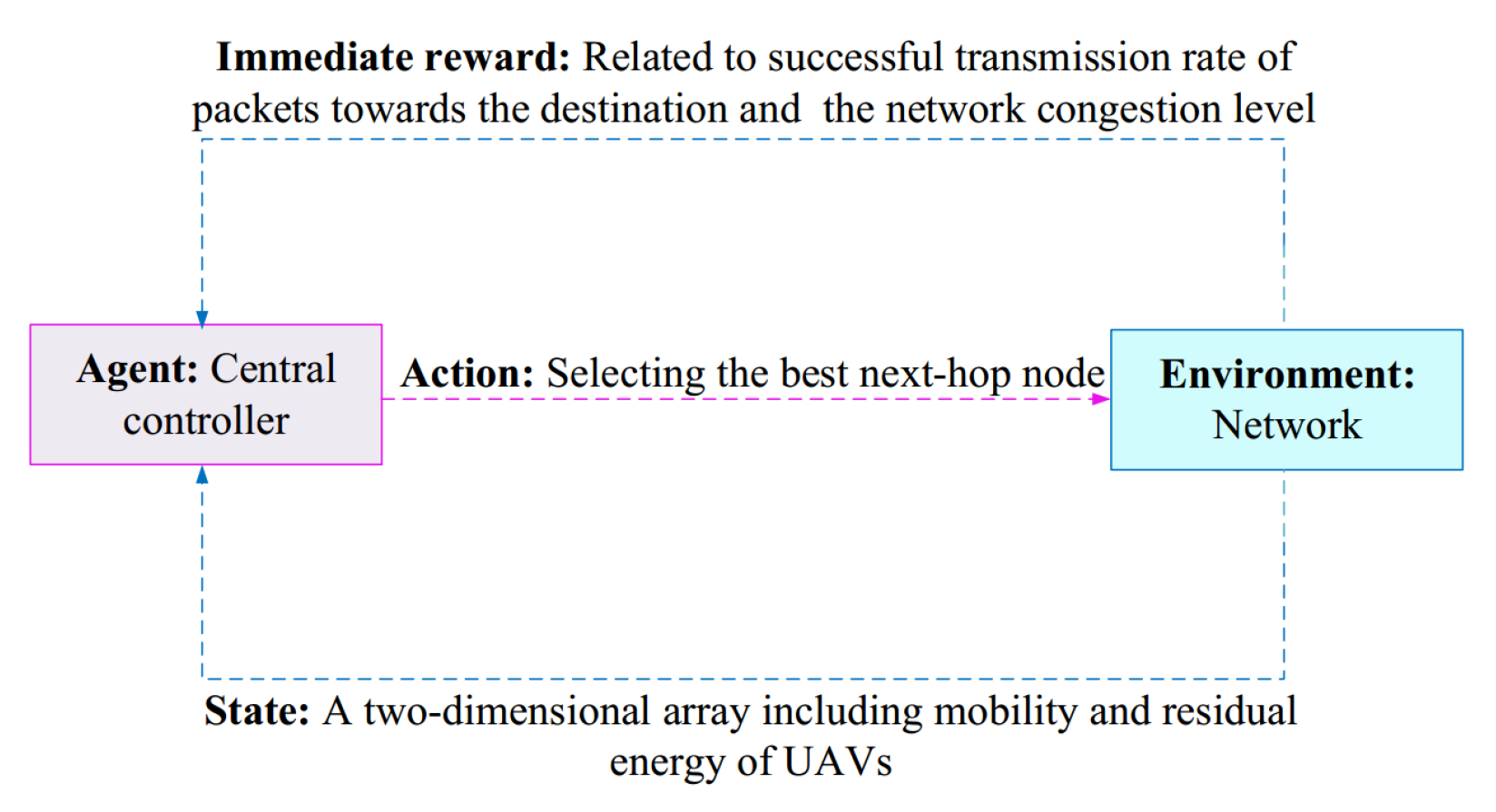
| DQN-VR [67] | DQN | Central controller | A 2D array, including mobility and residual energy | Selecting the best neighboring node | Related to the successful transmission rate and network congestion level | Fixed | Fixed |
| QTAR [68] | Q-learning | Each packet | Neighboring nodes towards destination | Selecting the best next-hop node | Related to delay, energy, and velocity | Based on two-hop delay | Related to the distance and velocity changes between a UAV and its neighbors |
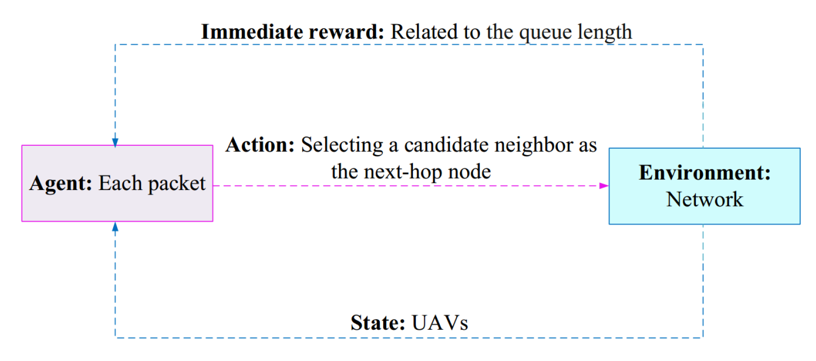
| TQNGPSR [69] | DQN | Each packet | UAVs | Selecting a candidate neighbor as the next-hop node | Based on the queuing length | Fixed | Fixed |
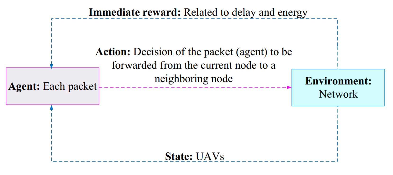
| QMR [70] | Q-learning | Each packet | UAVs | Decision of the packet (agent) to be forwarded from the current node to a neighboring node | Based on delay and energy | Based on single-hop delay | Related to the movement of neighbors in two consecutive intervals |
| QGeo [71] | Q-learning | Each packet | UAVs | Transition from transmitter to neighbor node | Related to packet travel speed | Fixed | Related to distance and the bobility pattern of UAVs |
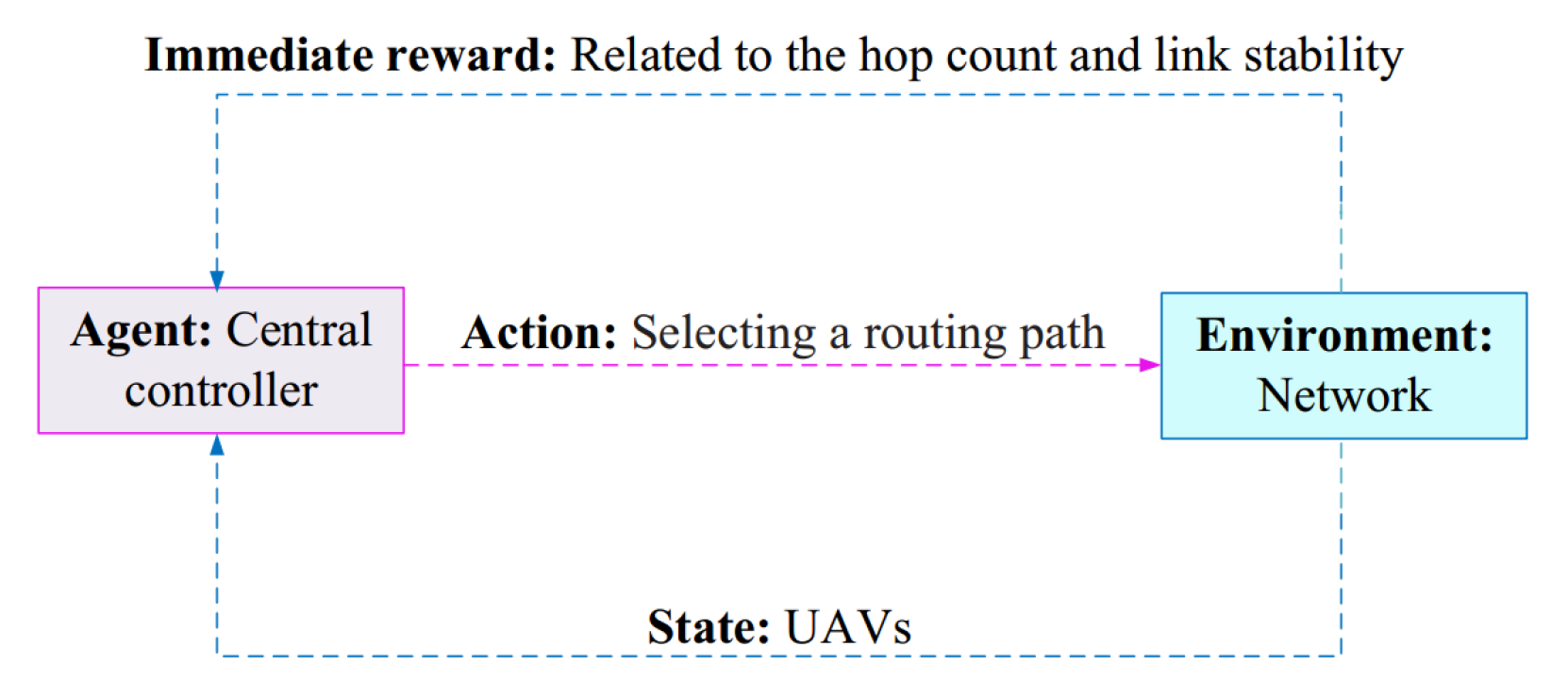
| QSRP [72] | Q-learning | Central controller | UAVs | Selecting a routing path | Related to link stability and hop count | Fixed | Fixed |
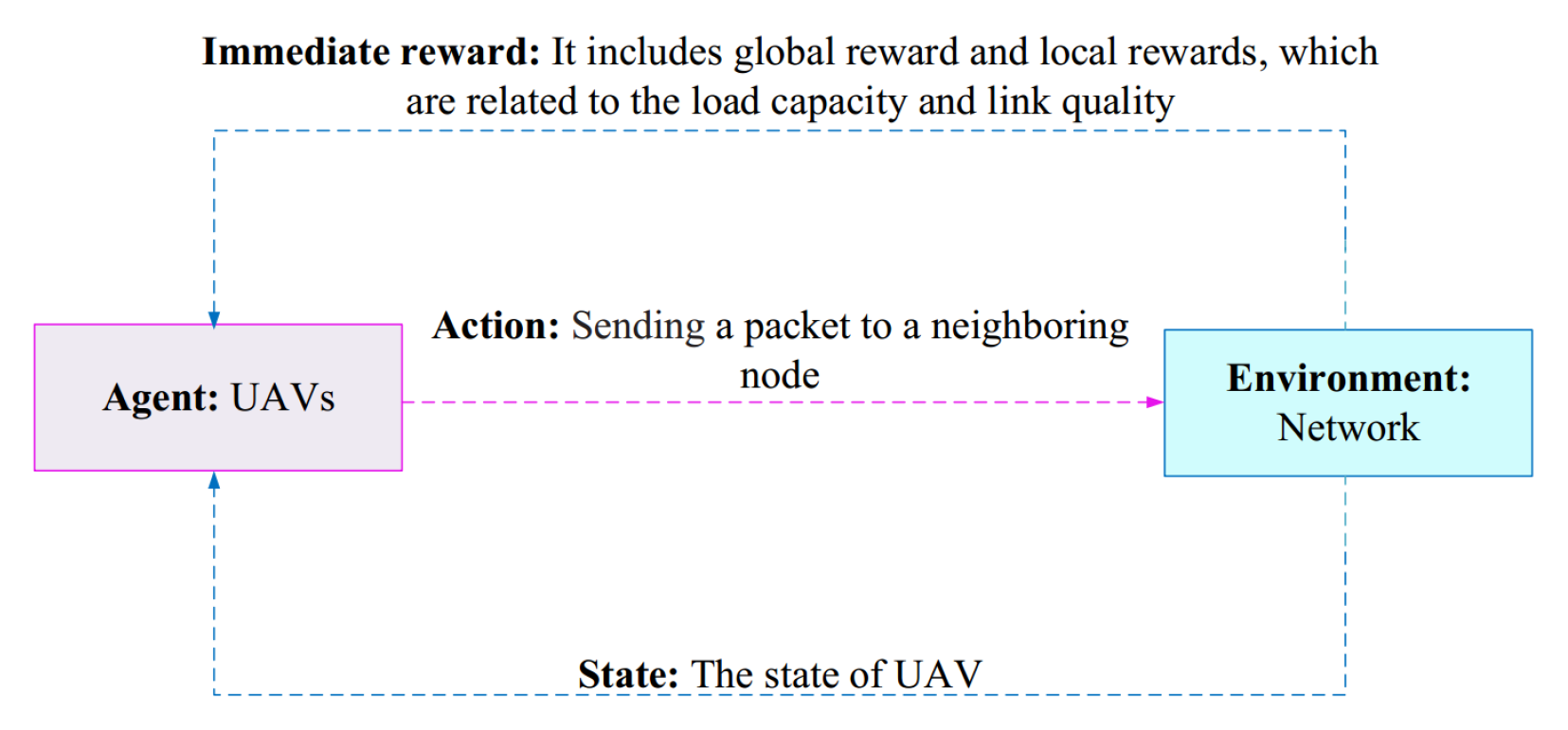
| QLGR [73] | Q-learning | UAVs | State of UAVs | Sending a packet to a neighboring node | Related to load capacity and link quality | Fixed | Fixed |
| FEQ-routing-SA [74] | Q-learning | Each UAV | State of UAVs | Sending a packet to a neighboring node | Related to transmission energy | Based on delivery time | Fixed |
| Q-FANET [75] | Q-learning+ | Each packet | UAVs | Sending the packet to a neighboring node | 100, if reaching the destination; , if trapping in a local optimum; 50, otherwise | Fixed | Fixed |
| PPMAC+RLSRP [76] | Q-learning | Each UAV | The state of UAVs | Sending the packet to a neighboring node | Related to transmission delay | Fixed | Fixed |
| PARRoT [77] | Q-learning | Each UAV | The state of UAVs | Selecting a neighboring node as the next-hop node | Related to reverse path score | Fixed | Based on the link expiry time (LET) and the change degree of neighbors |
| QFL-MOR [78] | Q-learning | Unknown | UAVs | Selecting a neighboring node as the next-hop node | Unknown | Fixed | Fixed |
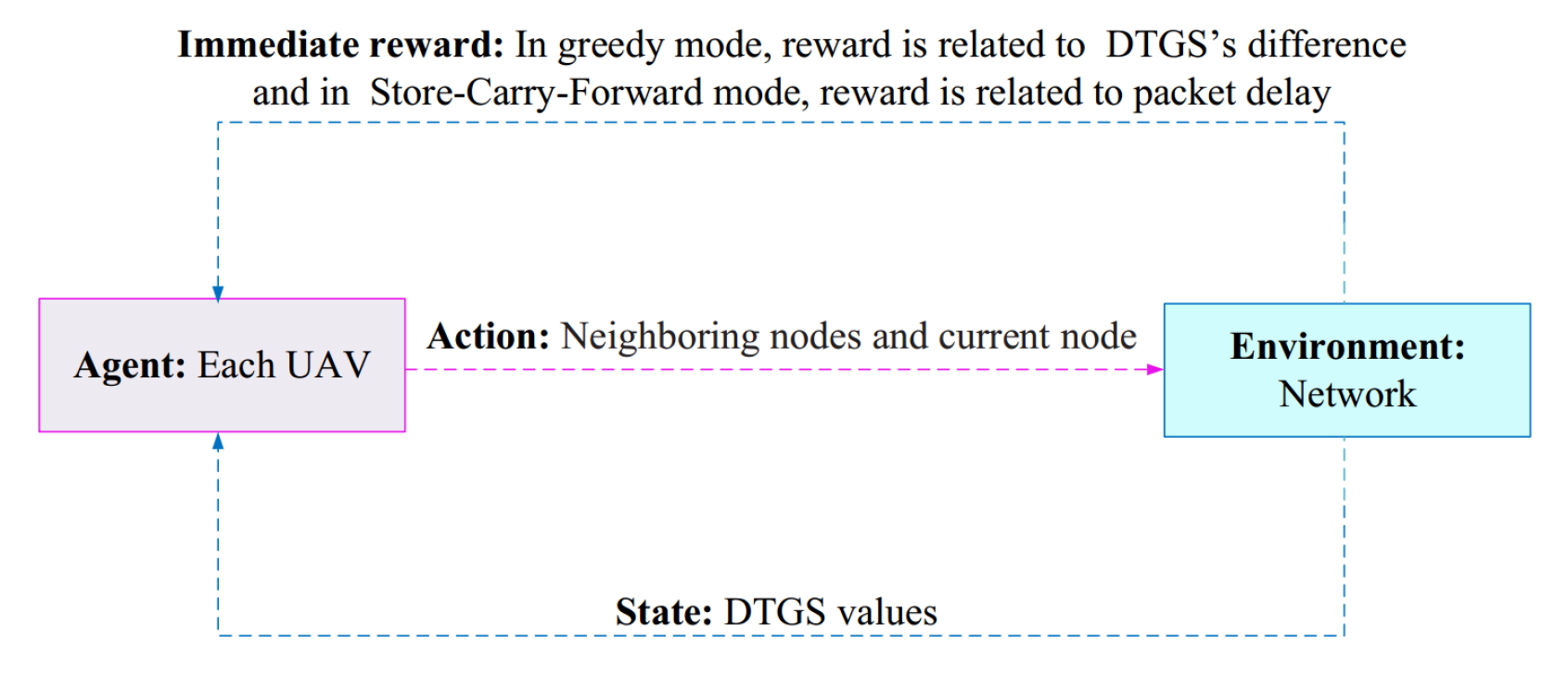
| 3DQ [79] | Q-learning | Each UAV | DTGS corresponding to neighboring nodes | Neighboring nodes and current node | The first function is related to DTGS difference; the second function is calculated based on packet delay | Fixed | Fixed |
| ICRA [80] | Q-learning | Ground station | Four utility factours | Weights of four utility factors | Related to cluster structure stability and the energy change rate | Fixed | Fixed |
| TARRAQ [81] | Q-learning | Each packet | UAVs | Selecting the next hop from neighboring nodes | Related to link quality, residual energy, and distance | Related to resigual link duration | Related to resigual link duration |
| Scheme | Reinforcement Learning | Deep Reinforcement Learning | ||||||
|---|---|---|---|---|---|---|---|---|
| Single-Agent | Multi-Agent | Model-Based | Free-Model | Single-Agent | Multi-Agent | Model-Based | Free-Model | |
| DQN-VR [67] | × | × | × | × | ✓ | × | × | ✓ |
| QTAR [68] | ✓ | × | × | ✓ | × | × | × | × |
| TQNGPSR [69] | × | × | × | × | ✓ | × | × | ✓ |
| QMR [70] | ✓ | × | × | ✓ | × | × | × | × |
| QGeo [71] | ✓ | × | × | ✓ | × | × | × | × |
| QSRP [72] | ✓ | × | × | ✓ | × | × | × | × |
| QLGR [73] | × | ✓ | × | ✓ | × | × | × | × |
| FEQ-routing-SA [74] | ✓ | × | × | ✓ | × | × | × | × |
| Q-FANET [75] | ✓ | × | × | ✓ | × | × | × | × |
| PPMAC+RLSRP [76] | ✓ | × | × | ✓ | × | × | × | × |
| PARRoT [77] | ✓ | × | × | ✓ | × | × | × | × |
| QFL-MOR [78] | ✓ | × | × | ✓ | × | × | × | × |
| 3DQ [79] | ✓ | × | × | ✓ | × | × | × | × |
| ICRA [80] | ✓ | × | × | ✓ | × | × | × | × |
| TARRAQ [81] | ✓ | × | × | ✓ | × | × | × | × |
| Scheme | Single-Path | Multi-Path |
|---|---|---|
| DQN-VR [67] | ✓ | × |
| QTAR [68] | ✓ | × |
| TQNGPSR [69] | ✓ | × |
| QMR [70] | ✓ | × |
| QGeo [71] | ✓ | × |
| QSRP [72] | ✓ | × |
| QLGR [73] | ✓ | × |
| FEQ-routing-SA [74] | ✓ | × |
| Q-FANET [75] | ✓ | × |
| PPMAC+RLSRP [76] | ✓ | × |
| PARRoT [77] | × | ✓ |
| QFL-MOR [78] | ✓ | × |
| 3DQ [79] | ✓ | × |
| ICRA [80] | ✓ | × |
| TARRAQ [81] | ✓ | × |
| Scheme | Flat | Hierarchical |
|---|---|---|
| DQN-VR [67] | × | ✓ |
| QTAR [68] | ✓ | × |
| TQNGPSR [69] | ✓ | × |
| QMR [70] | ✓ | × |
| QGeo [71] | ✓ | × |
| QSRP [72] | ✓ | × |
| QLGR [73] | ✓ | × |
| FEQ-routing-SA [74] | ✓ | × |
| Q-FANET [75] | ✓ | × |
| PPMAC+RLSRP [76] | ✓ | × |
| PARRoT [77] | ✓ | × |
| QFL-MOR [78] | ✓ | × |
| 3DQ [79] | ✓ | × |
| ICRA [80] | × | ✓ |
| TARRAQ [81] | ✓ | × |
| Scheme | Greedy | Store-Carry-Forward | Route Discovery |
|---|---|---|---|
| DQN-VR [67] | × | × | ✓ |
| QTAR [68] | × | × | ✓ |
| TQNGPSR [69] | ✓ | × | × |
| QMR [70] | × | × | ✓ |
| QGeo [71] | × | × | ✓ |
| QSRP [72] | × | × | ✓ |
| QLGR [73] | ✓ | × | × |
| FEQ-routing-SA [74] | × | × | ✓ |
| Q-FANET [75] | × | × | ✓ |
| PPMAC+RLSRP [76] | ✓ | × | × |
| PARRoT [77] | ✓ | × | × |
| QFL-MOR [78] | × | × | ✓ |
| 3DQ [79] | ✓ | ✓ | × |
| ICRA [80] | ✓ | × | × |
| TARRAQ [81] | × | × | ✓ |
| Scheme | Centralized | Distributed |
|---|---|---|
| DQN-VR [67] | ✓ | ✓ |
| QTAR [68] | × | ✓ |
| TQNGPSR [69] | × | ✓ |
| QMR [70] | × | ✓ |
| QGeo [71] | × | ✓ |
| QSRP [72] | ✓ | × |
| QLGR [73] | × | ✓ |
| FEQ-routing-SA [74] | × | ✓ |
| Q-FANET [75] | × | ✓ |
| PPMAC+RLSRP [76] | × | ✓ |
| PARRoT [77] | × | ✓ |
| QFL-MOR [78] | × | ✓ |
| 3DQ [79] | × | ✓ |
| ICRA [80] | ✓ | ✓ |
| TARRAQ [81] | × | ✓ |
| Scheme | Unicast | Multicast | Broadcast | Geocast |
|---|---|---|---|---|
| DQN-VR [67] | ✓ | × | × | × |
| QTAR [68] | × | × | ✓ | × |
| TQNGPSR [69] | ✓ | × | × | × |
| QMR [70] | × | × | ✓ | × |
| QGeo [71] | × | × | ✓ | × |
| QSRP [72] | × | × | ✓ | × |
| QLGR [73] | × | × | ✓ | × |
| FEQ-routing-SA [74] | ✓ | × | × | × |
| Q-FANET [75] | × | × | ✓ | × |
| PPMAC+RLSRP [76] | × | × | ✓ | × |
| PARRoT [77] | × | × | ✓ | × |
| QFL-MOR [78] | × | × | ✓ | × |
| 3DQ [79] | ✓ | × | × | × |
| ICRA [80] | ✓ | × | ✓ | × |
| TARRAQ [81] | × | × | ✓ | × |
Publisher’s Note: MDPI stays neutral with regard to jurisdictional claims in published maps and institutional affiliations. |
© 2022 by the authors. Licensee MDPI, Basel, Switzerland. This article is an open access article distributed under the terms and conditions of the Creative Commons Attribution (CC BY) license (https://creativecommons.org/licenses/by/4.0/).
Share and Cite
Lansky, J.; Ali, S.; Rahmani, A.M.; Yousefpoor, M.S.; Yousefpoor, E.; Khan, F.; Hosseinzadeh, M. Reinforcement Learning-Based Routing Protocols in Flying Ad Hoc Networks (FANET): A Review. Mathematics 2022, 10, 3017. https://doi.org/10.3390/math10163017
Lansky J, Ali S, Rahmani AM, Yousefpoor MS, Yousefpoor E, Khan F, Hosseinzadeh M. Reinforcement Learning-Based Routing Protocols in Flying Ad Hoc Networks (FANET): A Review. Mathematics. 2022; 10(16):3017. https://doi.org/10.3390/math10163017
Chicago/Turabian StyleLansky, Jan, Saqib Ali, Amir Masoud Rahmani, Mohammad Sadegh Yousefpoor, Efat Yousefpoor, Faheem Khan, and Mehdi Hosseinzadeh. 2022. "Reinforcement Learning-Based Routing Protocols in Flying Ad Hoc Networks (FANET): A Review" Mathematics 10, no. 16: 3017. https://doi.org/10.3390/math10163017