Article

A Non-Invasive Method to Evaluate Fuzzy Process Capability Indices via Coupled Applications of Artificial Neural Networks and the Placket–Burman DOE

by
Iván E. Villalón-Turrubiates
1,
Rogelio López-Herrera
1,
Jorge L. García-Alcaraz
2,
José R. Díaz-Reza
3,
Arturo Soto-Cabral
4,
Iván González-Lazalde
4,
Gerardo Grijalva-Avila
5 and
José L. Rodríguez-Álvarez
1,6,*
1
Department of Doctoral Program in Engineering Sciences, Western Institute of Technology and Higher Education, Tlaquepaque 45604, Mexico
2
Department of Industrial Engineering, Autonomous University of Ciudad Juárez, Ciudad Juárez 32310, Mexico
3
Division of Research and Postgraduate Studies, National Technology of Mexico, Technological Institute of Ciudad Juárez, Ciudad Juárez 32310, Mexico
4
Department of Industrial Engineering, National Technology of México, Technological Institute of Durango, Durango 34080, Mexico
5
Department of Manufacturing Engineering, Polytechnic University of Durango, Durango 34306, Mexico
6
Department of Management Engineering, National Technology of México, Higher Technological Institute of the Los Llanos Region, Guadalupe Victoria 34700, Mexico
*
Author to whom correspondence should be addressed.
Mathematics 2022, 10(16), 3000; https://doi.org/10.3390/math10163000
Submission received: 30 July 2022 / Revised: 10 August 2022 / Accepted: 13 August 2022 / Published: 19 August 2022

Abstract

:
The capability analysis of a process against requirements is often an instrument of change. The traditional and fuzzy process capability approaches are the most useful statistical techniques for determining the intrinsic spread of a controlled process for establishing realistic specifications and use for comparative processes. In the industry, the traditional approach is the most commonly used instrument to assess the impact of continuous improvement projects. However, these methods used to evaluate process capability indices could give misleading results because the dataset employed corresponds to the final product/service measures. This paper reviews an alternative procedure to assess the fuzzy process capability indices based on the statistical methodology involved in the modeling and design of experiments. Firstly, a model with reasonable accuracy is developed using a neural network approach. This model is embedded in a graphic user interface (GUI). Using the GUI, an experimental design is carried out, first to know the membership function of the process variability and then include this variability in the model. Again, an experimental design identifies the improved operating conditions for the significative independent variables. A new dataset is generated with these operating conditions, including the minimum error reached for each independent variable. Finally, the GUI is used to get a new prediction for the response variable. The fuzzy process capability indices are determined using the triangular membership function and the predicted response values. The feasibility of the proposed method was validated using a random data set corresponding to the basis weight of a papermaking process. The results indicate that the proposed method provides a better overview of the process performance, showing its true potential. The proposed method can be considered non-invasive.

1. Introduction

Statistical process control (SPC) is one of the methods most used in manufacturing industries to evaluate, monitor, and identify changes for process improvements. Thus, it is key to improving product quality and ensuring statistical process control [1,2]. The Shewhart control chart is a well-known, powerful method to examine the steadiness of a process. The control chart is a procedure to study a process from a sequence of random samples taken from the process. Data presented in the form of a control chart basis, patterns of runs, presence of outliers in the data will often suggest areas of opportunity for process improvement. Troubleshooting is successful when providing information about when the trouble began and what may be the cause. The process capability is independent of any specification; it represents the natural behavior of the process after the unnatural interferences are eliminated. It is a natural occurrence and is measured by the in-control chart variation. For these purposes, the traditional control technique introduced in 1924 by Walter Shewhart has been widely used in the manufacturing and service industries [3,4,5,6,7].
Monitoring whether the process is in statistical control has been the primary function of the control charts. They are based on data representing one or several products or service quality characteristics [2]. The variable control charts must be used if these characteristics are measured based on numerical scales. On the other hand, attribute control charts must be used if the quality characteristic cannot be easily represented in numerical form. However, for at least three decades, trends in research have dealt with the issue of control charts based on the fuzzy set theory [8,9,10,11], and this approach is still widely used [12,13,14,15,16].
Process capability analysis is another SPC tool, where process capability is very well defined as the capacity of a process to meet customer expectations defined as specification limits [17]. Process capability indices are summary statistics that measure the process characteristics overall or potential performance (variables or attributes) relative to the target and specification limits [18]. This approach helps define a relationship between the process capability and the specification limits. This correspondence is made by forming the width ratio between the specification limits and the natural width tolerance set as six process standard deviation units [19].
The main outputs for any process capability analysis will define whether a process can produce items within the specification limits predetermined by the customer. A larger value of the process capability index implies a high process yield; a lower one implies a low process yield. This process only expresses its capability at the moment and should never be considered capability in the future [20]. The typical process capability indices in the literature are C p , C p k , C p m , and C p m k [21]. In this research, the C p and C p k are only analyzed.
The C p index, called in literature as precision index [22], is defined as the ratio between specifications limits over the process spread ( 6 σ ) [17]. The index represents how well the process fits upper and lower specifications limits, describing the customer product requirements. When the process variation is considerable, the C p value is small, which means a poor process capability. Since this index never considers any process shift, if the process average is not centered near the midpoint of specification width, then the C p index could give misleading process performance. So, a new process capability index called C p k was introduced by Kane in 1986 [22]. The main use of the C p k index is to indicate the variability associated with a process. This index is widely used to relate the natural tolerances (3 σ ) to the customer requirements by considering the location of the process mean. Like to C p index, a greater value for C p k index is desired. A C p k index value greater or equal to 1.33 is recommended [23]. However, the C p and C p k indices are not related to the cost of failing to meet the customer’s target requirement. On the other hand, the C p m index introduced by Hsiang and Taguchi (1985) measures a process’s ability to cluster around the target and reflects the degree of process targeting [24]. However, the information provided by C p m index could be taken when the C p and C p k indices values are the same [19].
Because the fuzzy set theory introduced by Zadeh (1965) [25] has demonstrated to deal with imprecise information, its capability to determine flexible parameters and to analyze the results shows more sensitiveness [26], the fuzzy approach has received attention for the last two decades. Several studies that include the fuzzy set theory to calculate process capability indices can be found in the literature [1,2,26,27,28,29,30,31,32,33,34,35,36,37,38,39,40,41,42,43,44,45,46,47,48]. Since the introduction of neutrosophic logic (an extension of fuzzy logic), it has also been used to calculate process capability indices [49,50,51].
It is common to use a dataset collected from quality control laboratories or directly from automated measuring instruments that are part of the process to evaluate process performance. The process capability indices are the typical approach to deal with this task. Note that these standard methods use data taken on the final product.
However, for complex processes where it is challenging to have enough data to calculate process capability indices (under a traditional or fuzzy approach), an alternative method to gather the required data is based on developing models with sufficient predictive capability. This alternative is the use of neural networks-based predictive models that could work as a source of data when a reasonable accuracy has been reached. A wide range of these kinds of models can be found in the literature with application in different fields of science [52,53,54,55,56,57,58,59,60,61,62].
An alternative to the artificial neural network models is the neural structures based on the Geometric Transformation Model as a universal approximator. This approach uses a single methodological framework for various tasks. A fast non-iterative study with a predefined number of computation steps provides repeatability for large and small training samples [63]. Additionally, the neuro-fuzzy models are becoming more widespread in several industries. Tkachenko et al. (2021) [64] present a new neuro-fuzzy diagnostic system based on non-iterative ANN and a new fuzzy model, a T-controller.
Because the desired results for process capability indices are of the “bigger is better” type and considering that the process location and variability are two critical parameters in any process performance analysis. The traditional experimental designs are a powerful tool to overcome this problem. This approach has been widely exploited in different fields of science to define optimal process conditions [65,66,67,68,69,70,71,72]. However, although the traditional design of experiments is very common, for almost two decades, the design of experiments approach has also been applied via couple with neural networks models [73,74,75,76,77,78,79,80,81,82].
This research presents a novelty method to evaluate process performance by a non-invasive approach to calculate the fuzzy process capability indices. The proposed method uses the significative process variables data records that influence the response. The data collected is used to develop an artificial neural network model. This model is now being employed as a data source, firstly applying it to the design of experiments approach to identify the optimal conditions for the process performance. Once the optimal variables operating values have been obtained, these new operating conditions are re-introduced to the neural network model to calculate the output measures. Measures that are being used to calculate the fuzzy process capability indices. Currently, an integral method like the one presented is not found in the literature. The main contributions of this study are described below.
  • Artificial neural network-based modeling with reasonable accuracy has been reached in a papermaking process. Hence, this model can be used to measure a critical quality characteristic.
  • The fuzzy set theory has been incorporated to overcome the vagueness and uncertainty in the generated data commonly presented in soft sensors.
  • Via coupled applications of artificial neural network based-modeling + experimental designs, data for process performance evaluation can be generated by engineers instead of taking measurements directly on the product. Hence, the method can be considered as non-invasive.
This paper is organized as follows: Section 2 briefly reviews the traditional and fuzzy methods to calculate process capability indices. Section 3 presents the proposed methodology by defining a framework. Meanwhile, Section 4 presents an actual case application presenting data from a papermaking process to validate the proposed method. Finally, the last section presents the conclusions and recommendations.

2. A Review of Fuzzy and Traditional Process Capability Indices

2.1. Traditional Process Capability Indices Cp and Cpk

The two most widely used standard process capability indices are C p and C p k . Known as traditional process capability indices, these are determined under the assumption that the process is in statistical control, which means that the variation is due only to random causes. In any process capability analysis using these indices, the response variable values are compared against specific limits and the customer specifications. The comparison is made by forming the width ratio between the specification limits and the natural tolerance width measured by six standard deviation units [19].
In the beginning, it was called the precision index [22], and the C p was the first process capability index to appear in the literature. This index is defined as the ratio of specifications width (USL-LSL) over the six sigma process spread [19,21]. This index is calculated by using Equation (1).
C p = A l l o w a b l e   P r o c e s s   S p r e a d A c t u a l   P r o c e s s   S p r e a d = U S L L S L 6 σ
where USL and LSL are the upper and lower specification limits, respectively, while σ is the standard deviation of the process.
Because C p focuses on the process dispersion, and this index does not consider the centering of the process [17], the C p k index is being used to overcome this problem. C p k relates the natural process tolerance ( 3 σ ) to the specification limits. It is used to describe how well the process fits within the specification limits by considering the location parameter (mean). This index is calculated by using Equations (2)–(4) [19,21,22].
C p k = min [ C p l , C p u ]
C p l = ( μ L S L ) 3 σ
C p u = ( μ U S L ) 3 σ

2.2. Fuzzy Process Capability Indices with Triangular Fuzzy Numbers

The fuzzy process capability indices are calculated using different membership functions to generate the fuzzy numbers. However, this study is based on the fuzzy process capability indices using the triangular fuzzy numbers approach, as described by Kaya and Kahraman in 2010 [18].
When a process capability analysis is based on a fuzzy approach, then a fuzzy estimator for σ 2 is essential. This fuzzy parameter is defined by the confidence interval shown in Equation (5).
[ n σ ^ 2 χ R , β / 2 2 , n σ ^ 2 χ L , β / 2 2 ]
where χ R , β / 2 2 , and χ L , β / 2 2 are the points on the right and left sides of the χ 2 Chi-square density function, respectively. Where the probability of exceeding the corresponding limit is β / 2 . However, this formula is a biased estimator for the variation ( σ 2 ). Equation (6) is defined to calculate an unbiased fuzzy estimator.
L ( λ ) = [ 1 λ ] χ R , 0.005 2 + λ n ,   R ( λ ) = [ 1 λ ] χ L , 0.005 2 + λ n
The unbiased ( 1 β ) × 100% confidence interval for σ 2 should be calculated from Equation (7).
L σ ^ ˜ c = [ n σ ^ 2 L ( λ ) , n σ ^ 2 R ( λ ) ] , 0 λ 1
Suppose the β parameter is considered as α-cut level. In that case, the fuzzy triangular membership function for σ 2 is obtained from Equation (7) and described in Equation (8). Therefore, the triangular membership functions can be developed by placing the previous confidence intervals on top of each other.
( σ ^ c ) α = [ n σ ^ 2 [ 1 α ] χ R , β / 2 2 + n α , n σ ^ 2 [ 1 α ] χ L , β / 2 2 + n α ] , 0 α 1
when the fuzzy estimator for σ 2 has been determined, it is possible to establish specification limits as triangular fuzzy numbers (TFN). Assume that the upper and lower specification limits (USL and LSL) are defined as: U S ˜ L = ( u 1 , u 2 , u 3 ) , and L S ˜ L = ( l 1 , l 2 , l 3 ) .
These limits are calculated by including the α-cuts, as shown in Equation (9) and Equation (10), respectively.
U S ˜ L α = [ ( u 2 u 1 ) α + u 1 , ( u 2 u 3 ) α + u 3 ]
L S ˜ L α = [ ( l 2 l 1 ) α + l 1 , ( l 2 l 3 ) α + l 3 ]
Now, it is possible to calculate the process capability indices. To calculate the fuzzy C p , Equation (11) is used. And to estimate the fuzzy C p k , the Equations (12)–(14) are being used.
( C ^ ˜ p c ) α = ( [ ( u 2 u 1 ) + ( l 3 l 2 ) ] α + ( u 1 l 3 ) 6 n σ ^ 2 ( 1 α ) χ L , β / 2 2 + ( α n ) , [ ( u 2 u 3 ) ( l 2 l 1 ) ] α + ( u 3 l 1 ) 6 n σ ^ 2 ( 1 α ) χ R , β / 2 2 + ( α n ) )
( C ˜ p u c ) α = ( [ ( u 2 u 1 ) α + u 1 ] μ 3 n σ ^ 2 ( 1 α ) χ L , β / 2 2 + ( α n ) , [ ( u 2 u 3 ) α + u 3 ] μ 3 n σ ^ 2 ( 1 α ) χ R , β / 2 2 + ( α n ) )
( C ˜ p l c ) α = ( μ [ ( l 2 l 3 ) α + l 3 ] 3 n σ ^ 2 ( 1 α ) χ L , β / 2 2 + ( α n ) , μ [ ( l 2 l 1 ) α + l 1 ] 3 n σ ^ 2 ( 1 α ) χ R , β / 2 2 + ( α n ) )
C ˜ p k c = min { C ˜ p u c , C ˜ p l c }

3. Methodology

This section describes the proposed method to evaluate the fuzzy process capability indices. The model and the graphic user interface developed by Rodriguez et al. [83] are used to generate data. The validation is only presented for the experimental designs and process capability indices steps.

3.1. Modeling

For any dataset in a science project, it is essential to understand how the data have been collected, stored, transformed, reported, and used [84]. Furthermore, understanding the range of factors to consider about manufacturing process data is mainly related to the quality and availability of the data, gaps in the data, or lack of data. Depending on the application, the manufacturing process data are stored in different repositories, including public and commercially available databases and private collections [85].
The more significant time-consuming part of the data science process is preparing the dataset to suit a data science task [84]. Dataset is rarely structured and available in the form required. Most data science algorithms require data to be structured in a tabular format with records in the rows and variables in the columns. When the data is presented in any other form, the dataset may need to be transformed into the required structure.
Before conducting an in-depth analysis of the data, exploring the dataset is another essential task. Also known as exploratory data analysis, which is probably the most time-demanding task of data preparation. This task uses a set of simple tools to understand the data and involves computing descriptive statistics and data visualization [84]. This task can expose the structure of the data, the distribution of the values, the presence of outlier values, and highlight relationships whiting the dataset. In addition, descriptive statistics like mean, median, mode, standard deviation, and range for each independent variable provide an easily readable summary of the key characteristics. Furthermore, the parameters could be used in the data imputation process.
Finally, an in-depth data analysis is performed to find a model to predict a variable of interest. A model is the abstract representation of the data and the relationships in a given dataset.
There are a few hundred data science algorithms in use, derived from statistics, machine learning, pattern recognition, and the body of knowledge related to computer science. Fortunately, many viable commercial and open-source data science tools are on the market to automate the execution of these learning algorithms.
As in the present study, classification and regression are commonly used to predict an outcome result based on one or more input variables. However, artificial neural networks have been widely used in many applications [85] due to their potential for predictive purposes.

3.2. Graphic User Interface

Currently, most intelligent computing devices use graphic user interfaces to reduce user learning curves and better interact with the process [86].
In any development process of a graphic user interface, the interface and interaction design take up most of the time in software use. Although there are many types of GUI’s, typically, this tool is composed of two main categories: the containers that represent the menu and the controls that represent the basic objects of the user interaction [87]. A common GUI development approach is presented by Monte-Mor et al. (2011) [88].
This study presents the model deployment presented by Rodriguez et al. in a graphic user interface as an interactive soft sensor shown by Rodríguez et al. [83].

3.3. Experimental Designs

The main reason for using experimental designs is their ability to provide evidence of causality [89,90,91]. The power of experiments to establish cause and effect relationships is critical to developing knowledge in any field of science [92]. The literature has referred to experimental designs as the gold standard of scientific research [93,94,95]. Moreover, other studies have noted the importance of experimental designs for testing theoretical concepts and how people better understand the world [96,97,98]. Therefore, the main goal of the experimental designs is to determine the causal relationships between independent and dependent variables.
The proposed method includes the experimental designs as one of the main steps to evaluate the process capability indices. However, the experimental design is carried out as a no-invasive approach [99]. Furthermore, the proposed method suggests using the most common experimental design approaches: screening, factorial, response surface, mixture, and Taguchi. But the approach used will depend on the specific research objective. This study uses a Placket-Burman factorial design.

3.4. Generate Data

Generally, any process capability analyses are carried out using data from quality control laboratories or the measures taken from the quality control system. Several studies can be found where traditional and fuzzy approaches are used to calculate process capability indices. However, in the present work, the data are taken using the previously developed interactive soft sensor.
Before generating data for the process capability analysis, the optimal operation conditions determined by the experimental design step are considered. However, the values found in the experimental designs are ideal ones. Although, it is complicated to maintain a fixed set point in the process. It is fundamental to determine the variability of the independent variables in the process.
Thus, the variability for all independent variables is firstly determined. This variability generates random data around the set point (previously found optimal condition). The amount of data generated is based on cycle time and the process capability to store data.

3.5. Process Capability Indices

If the generated data follows a normal distribution, then the process capability indices can be well estimated using the traditional approach. However, as the proposed method uses predicted data, the data will probably show uncertainty. Therefore, the fuzzy process capability analysis is the better option.
In this study, the process capability analyses presented in [17] are applied to a papermaking process. Figure 1, is shown the proposed method called the “non-invasive method to evaluate the fuzzy process capability indices” (Non-I FPCA).

4. Real Case Application

The process capability analysis has been held for a papermaking process in a paper grade of 200 g (basis weight named “L-200”). These capability indices have been calculated using a fuzzy environment to get more reliable information about the process capability.
Firstly, the model proposed in [83] is used as an alternative method to collect data on paper’s basis weight. This model is advantageous since it can predict the basis weight with reasonable accuracy (greater than 90%) for new operating conditions or data not included in the training and validation process. Mainly for the grades from 180 to 250 g/m2, reaching an error from 4.8 to 6.7%. In the modeling process, the input array size was 182,834 rows by 24 columns, while the output array size was 182,834 rows by one column. This amount of data samples was enough to develop a robust neural network model. Additionally, the 24 columns correspond to all the independent variables affecting the basis weight in the paper. Hence, these variables must be continuously monitored and controlled by process engineers.
For the training and validation process, the input array size was 164,550 rows by 24 columns, while the output array size was 164,550 rows by one column. In the testing process, the input array size was 18,284 rows by 24 columns, while the output array size was 18,284 rows by one column. The following is a more detailed description of the process of obtaining the neural network model proposed in [83].
The best-found architecture and structure of the neural network model are shown in Table 1. The activation functions and the number of neurons per layer were moved by trial and error for the neural network architecture design. Meanwhile, the rest of the hyperparameters were: the loss and metric functions, a learning rate of 0.001 for the RMSprop optimizer, a batch size of 32, and 1000 epochs for each of the training and test process.
Figure 2 presents a training summary for the model loss level. Meanwhile, in Figure 3 is shown the predicted vs. test data to evaluate the model performance in the building process. Finally, in Figure 4 is shown in detail the predicted vs. test data for a random range selected from 12,000 to 12,200. As shown in graphical results, the model developed can determine the basis weight with reasonable precision.
The resulting mean absolute error (MAE) was 12.40 g. In addition, an external dataset not included in the process building of the model was used to validate the model performance. The resulting mean absolute error (MAE) was 12.10 g by using the external dataset.
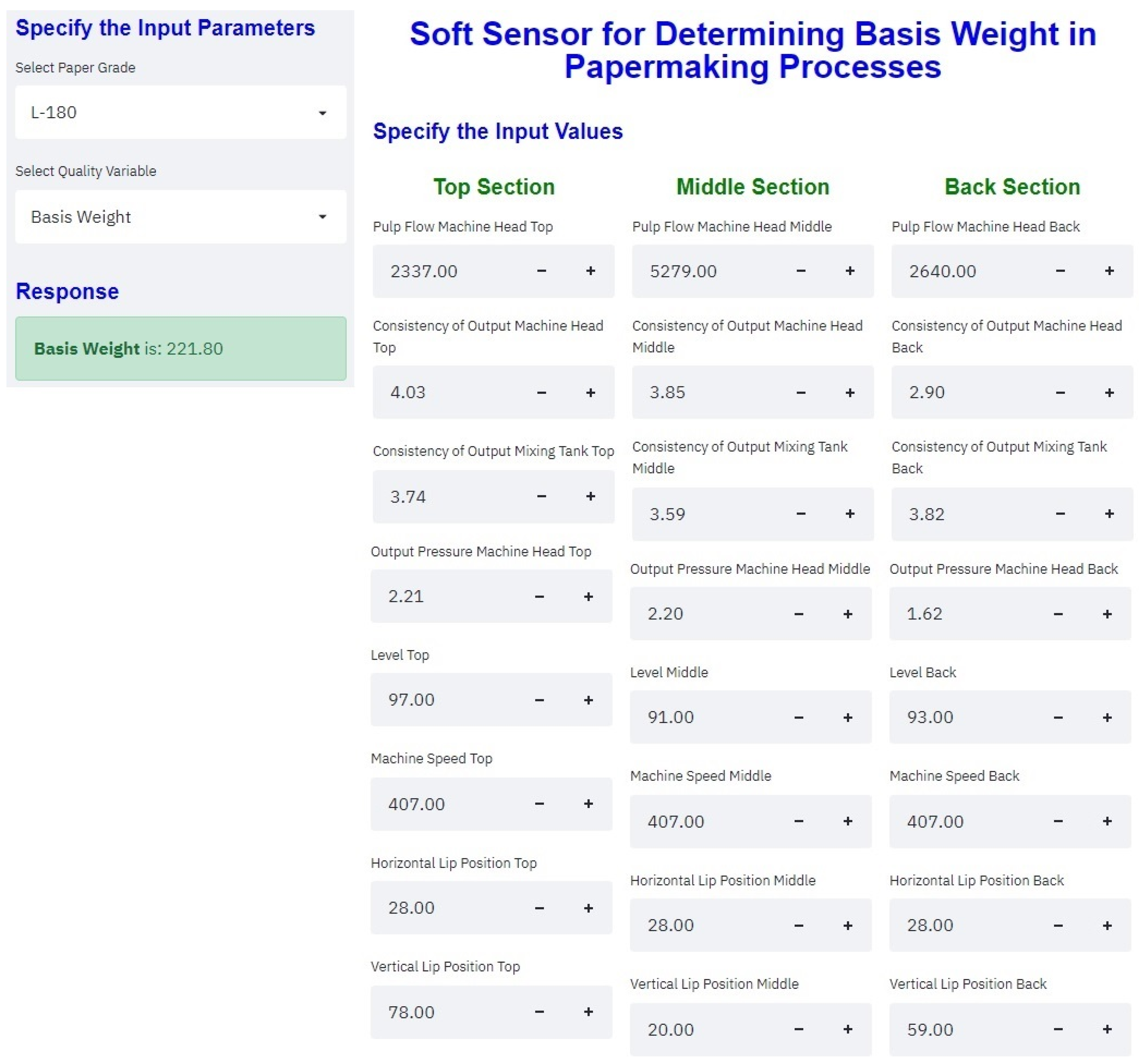
The graphic user interface was developed using the streamlit library in the Python programming language. So, the model was embedded in the user interface. The generated package can work well in any local host. Moreover, the model can also work in a web environment, allowing the process engineers to calculate basis weight offline. Figure 5 shows the framework of the graphic user interface proposed by Rodríguez et al. [83]. To present the graphical user interface from a terminal on your computer, you must add the path where the GUI source code is located and then enter the following instruction: run streamlit name.py.
The GUI will automatically display the average value of each independent variable; however, as mentioned above, the user can manually manipulate each variable.
Given the excellent performance shown by the neural network model to predict the basis weight, it was used to evaluate the response in the experimental design step. In addition, due to the large number of independent variables involved in the papermaking process, the Placket-Burman factorial experimental design was selected. Before carrying out the experimental design analysis, all independent variables were coded. The high and low levels of each independent variable were defined in collaboration with process engineers according to the parameters commonly used to manufacture the different grades of paper. Table 2 shows the entire list of independent variables and their levels included in the experiment.
Notice that the developed model is deterministic since the response will always be the same under the same operating conditions. However, in a real situation, the response must show variability. So, a first experimental design must be carried out to know the variability and include it in the model response. Therefore, Minitab-19® was used to generate the fully randomized design table. This table contains one replicate per experiment, with 48 runs without blocks. Each experiment’s response (basis weight) was the predicted value using the neural network model inserted in the graphic user interface. Notice that each run of the experimental design can be entered manually in the graphical user interface or enter all runs as a matrix array in the source code that generated the neural network model in Python using the model.predict(x) function. The coded data are presented in the Appendix A.
The results in Figure 6 show that the model’s assumptions are met: normality, constant variance, and independence. Meanwhile, Table 3 summarizes the analysis of variance. The stepwise selection method uses an α risk value to enter 0.15 and an α risk value to remove 0.15. The results indicate that the process variables, Pulp Flow at Machine Top, Pulp Flow at Machine Middle, Pulp Flow at Machine Back, Consistency at Machine Back, and Vertical Lip Position, were significant at 5%. On the other hand, Consistency at Machine Top, Level Middle, and Horizontal Lip Position Middle showed p-values of 0.051, 0.064, and 0.067, respectively. These variables were also considered significant. The main effects plot for each variable mentioned above is shown in Figure 7.
Note the main experimental design results are shown, such as the graphs validating the model assumptions, the analysis of variance, and the main effects plot. However, in the present work, the experimental design approach is used to obtain the optimal operating parameters (for a 200 g paper) for all 24 independent variables and not to quantify the effects on the response variable (basis weight).
Finally, the first optimal operating conditions were determined by using the response optimizer. The results show a desirability index of 1.000 and the optimal values are summarized in Table 4. Although these variables considerably affect the basis weight, defining the values (in advance, which are called set points) for the other independent variables is necessary. Therefore, Table 4 also presents the recommended values.
The next step is generating the data to know the expected fuzzy process variability. Thus, the variability for all independent variables is determined. This variability is shown in Table 4. This variability is included in a random dataset generated around the set point for each independent variable. Since the cycle time of a paper roll is about forty minutes, and because the papermaking process can generate data in the interval time of one minute; hence, a total of forty random data were generated for each independent variable. The resulting array size of 40 rows by 24 columns was introduced in the GUI to predict the basis weight. The predicted values (basis weight) used to calculate the fuzzy process variability are illustrated in Table 5. Finally, using Equation (8), the membership function of σ ^ c has been calculated and illustrated in Figure 8. The results show that the standard deviation ranges from 1.39 to 4.55. This variability was included in the developed model. So, the predicted values are now affected by any random value taken from this data range.
Because the developed model is capable to provide different basis weight values for the same provided operating conditions; therefore, it is possible to perform replicated experimental designs, which allow knowing the variability, magnitude, and direction of the effects for each independent variable. Thus, by following the same method mentioned above, Minitab-19® is used again to carry out a replicated experimental design. Firstly, a fully randomized design table is generated. This table contains five replicates per experiment; so, there are 240 runs without blocks. The generated matrix size is 240 rows and 24 columns (due to the table size, these data are not included in the paper). This matrix is used to estimate the basis weight for each experiment (operating condition).
The results in Figure 9 show that the model’s assumptions are again met: normality, constant variance, and independence. As mentioned above, the experimental design approach is used to obtain the optimal operating parameters; however, the tables shown in Appendix B and Appendix C summarize the coefficients and the analysis of variance, respectively. The results indicate that the process variables significant at a level of 5% were: Pulp Flow at Machine Top, Consistency at Machine Top, Pulp Flow at Machine Middle, Output Pressure at Machine Middle, Level Middle, Pulp Flow at Machine Back, Consistency at Machine Back, Consistency at Tank Back, Output Pressure at Machine Back, Level Back, Machine Speed Top, Ver Lip Position Top, Hor Lip Position Middle, and Ver Lip Position Middle. These variables have a significative effect on the basis weight. However, variables such as Pulp Flow at Machine Top, Consistency at Machine Top, Pulp Flow at Machine Middle, Level Middle, Consistency at Tank Back, Level Back, Machine Speed Top, Ver Lip Position Top, Hor Lip Position Middle, and Ver Lip Position Middle must be changed from low to a high level to reduce variability.
Meanwhile, the rest of the significative variables must change from high to low. The main effects plot for each variable mentioned above is shown in Figure 10. Finally, the optimal operating conditions were determined using the response optimizer in Minitab-19®. The results show a desirability index of 1.000 for the optimal values summarized in Table 6.
The following step is generating the data to carry out the fuzzy process capability analysis. Again, the expected variability for each independent variable (presented in Table 4) must be considered. Therefore, using this variability, a new random dataset is generated around the set point defined in Table 6. Note that the operating conditions shown in Table 6 differ from those in Table 4. This difference is because the model includes the previously calculated variation and will present variation in the output data similar to the shown by the measurement systems. Hence, the resulting array size was 40 rows by 24 columns in the step where the variability range was estimated. This matrix was introduced in the graphic user interface to predict the basis weight. The predicted values (basis weight) used to apply the fuzzy process capability analysis are illustrated in Table 7. Note that these values include the expected variation for each independent variable and the variability included in the model.
The fuzzy process capability indices are calculated in the proposed method’s last step. Firstly, using Equation (8), the membership function of σ ^ c has been calculated and illustrated in Figure 11. The standard deviation goes from 2.40 to 7.87 for different α -cut values. Notice that this variability is greater than estimated at the beginning because this variability includes the variability shown by all independent variables. This variability could be larger; however, by defining the optimal parameters, the variability was reduced in the predicted values of the basis weight. In addition, if the process engineers can have a better control for each of the significant critical variables identified in the experimental design step; then, the standard deviation would be reduced.
With σ ^ c calculated, now it is possible to calculate the fuzzy process capability indices. Because the method used to estimate σ ^ c included all data; therefore, C ^ ˜ p c and C ˜ p k c must be changed to P ^ ˜ p c and P ^ ˜ p k c . The specification limits are defined by using the triangular fuzzy numbers to achieve this aim. Since the upper and lower specification limits for a paper grade of 200 g are 210 and 190 g, respectively; therefore, the specification limits are defined as follows: U S ˜ L α = T F N ( 208 ,   210 ,   212 ) and L S ˜ L α = T F N ( 188 , 190 ,   192 ) .
Now, by using the Equations (9) and (10) the α -cut values for the upper and lower specification limits are obtained as follows: U S ˜ L α = [ 2 α + 208 , 2 α + 212 ] , and L S ˜ L α = [ 2 α + 188 , 2 α + 192 ] . And by using Equation (11), the membership function of P ^ ˜ p c is calculated and depicted in Figure 12. The range for P ^ ˜ p c goes from 0.54 to 1.19 with different α -cut values.
Equations (12) and (13) are used to calculate the membership functions of P ˜ p u c and P ˜ p l c . P ˜ p u c changes between 0.27 to 0.92 with different α-cut values. Meanwhile, P ˜ p l c changed between 0.69 to 1.68 with different α -cut values. Therefore, using Equation (14), the range for P ˜ p k c goes from 0.27 to 0.92, as shown in Figure 13.
The membership functions of σ -level were also calculated using the following equation: σ = 3 P ˜ p k c . The σ -level change between 0.81 to 2.77, as shown in Figure 14.
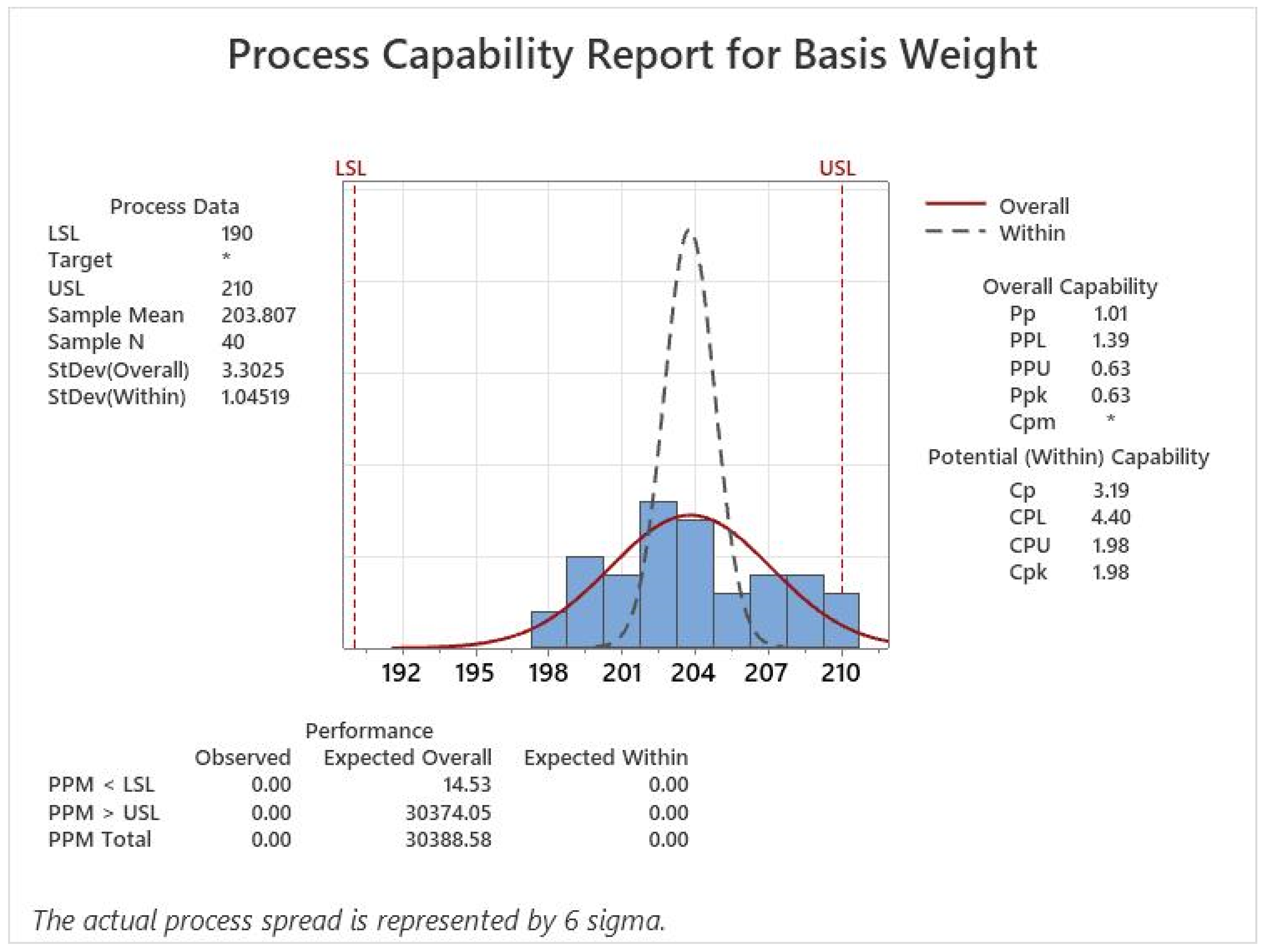
Finally, a dataset of 200 g of paper grade randomly selected from the quality control system (QCS) is collected to compare the proposed method against the traditional and fuzzy approaches. For this purpose, forty continued basis weight readings between 190 to 210 g were taken. The P p and P p k indices were calculated using the traditional process capability analysis. The used dataset is illustrated in Table 8. The analysis was carried out in Minitab-19®. The results show a P p of 1.01 and a P p k of 0.63, as shown in Figure 15. In addition, the fuzzy process capability indices were calculated for different α -cut values using the same dataset. The results show that the standard deviation goes from 2.02 to 6.61. The P ^ ˜ p c ranges go from 0.64 to 1.42, while the P ˜ p k c goes from 0.30 to 1.06. Finally, the σ -level changes between 0.90 to 3.17. These values are presented from Figure 11, Figure 12, Figure 13 and Figure 14, respectively.

5. Conclusions

Unlike the existing methods, the proposed method does not use final product/service measures. Instead, the used dataset corresponds to predicted values made by the trained model. Therefore, the fuzzy process capability indices are determined by using data directly from each independent variable that affects the response, including its variability.
In the traditional approach to evaluating process capability indices, the response variable values are usually close to the target value because the data come from a normal process. In the proposed method, the experimental designs were used first to know the membership function of the process variability. The standard deviation ranges from 1.39 to 4.55. The model included this variability to carry out a replicated experimental design to define the optimal operating conditions that will bring the response variable closer to a target value.
The P p and P p k capability indices estimated using the traditional approach are within the range of values calculated with the proposed method for these same indices. The results showed a P p of 1.01, and P p k of 0.63. When the minimum and maximum values are calculated with the proposed and existing fuzzy methods, the standard deviation with the proposed method will always be larger than the existing fuzzy methods. This difference is because the model includes the natural variation of the process and the variation shown by each independent variable. As shown in Figure 11, the proposed method showed a larger standard deviation than the fuzzy method. For this parameter, the proposed method showed values from 2.40 to 7.87, while the fuzzy method results showed values from 2.02 to 6.61. For the P ^ ˜ p c index, the proposed method showed a P ^ ˜ p c from 0.54 to 1.19, while the fuzzy method showed a P ^ ˜ p c from 0.64 to 1.42. Meanwhile, the proposed method showed a P ˜ p k c from 0.27 to 0.92, compared with the fuzzy method showing a P ˜ p k c from 0.30 to 1.06. On the other hand, the proposed method showed a σ -level from 0.81 to 2.77, while the fuzzy method showed values from 0.90 to 3.17.
Since most of the processes tend to maintain or even decrease their performance, and because the variability of the independent variables was included; therefore, the results indicate that the proposed method gives us a better overview than the traditional and fuzzy approaches related to the true potential of the process performance. The proposed method’s observed advantages come from finding the optimal operating conditions of the process parameters to obtain the desired result of the paper basis weight and reduce its variability.
An essential benefit of using the proposed method is that it allows us to know the impact on performance and variability of the significant variables of the paper manufacturing process; thus, this information should guide us in the product and process improvements.
Furthermore, this method is helpful for slow processes where cycle times are very long and collecting enough data to perform a process capability analysis is complicated. In addition, if data can be collected for each process variable, then the process capability indices can be calculated for each manufactured product/service.
On the other hand, since a variability factor is added around an optimal value defined in the experimental design step, the proposed method’s performance results will always present a different value even when using the same data collected for each independent variable. Therefore, this disadvantage will affect the variation of the intersection point probability. Finally, although the model can estimate the basis weight reasonably, general assumptions must be verified and this technology could be susceptible to measurement drift from long-term usage. Additionally, since the neural network model performance relies heavily on the historian data for specific paper grades. If there is a significant change in the paper included during the design, rebuilding the neural network model will be recommended.
Because the fuzzy process capability indices were estimated using the triangular membership function, the proposed method will use other fuzzy membership functions in future research to compare their results with reality. In addition, a sensitivity analysis could be performed in order to compare the results of the proposed model with other approaches such as the neuro-fuzzy systems and neural-like structures based on geometric data transformations.

Author Contributions

Conceptualization, supervision and validation, I.E.V.-T.; supervision and validation, J.L.G.-A.; conceptualization, supervision, and validation, R.L.-H.; validation, J.R.D.-R. and G.G.-A.; visualization, A.S.-C. and I.G.-L.; conceptualization, investigation, methodology, data curation, and writing—review and editing, J.L.R.-Á. All authors have read and agreed to the published version of the manuscript.

Funding

This work was partly supported by the National Council of Science and Technology (CONACYT) through a scholarship 487109 granted to J. L. Rodríguez-Álvarez.

Institutional Review Board Statement

The study did not require ethical approval.

Informed Consent Statement

Not applicable.

Data Availability Statement

Data available on request.

Conflicts of Interest

The authors declare no conflict of interest.

Appendix A. The Coded Data in the First Experimental Design

ABCDEFGHJKLMNOPQRSTUVWXYBW
15003.54.52.58555003.54.51.58520004.54.51.595473472472307525203060194.59
25003.53.51.59555003.54.52.58520004.53.51.595473473472307530152560189.61
25004.54.51.59545004.53.51.59530004.54.51.595473473473307525152560166.27
25003.53.52.59555003.54.51.59520003.54.52.595473472473308030202555203.37
25003.53.52.59555004.53.52.59530004.54.51.585472472473257525153060154.35
25004.54.51.58545003.54.51.58520003.54.52.585473472473257525203055197.43
15004.54.52.58555003.54.51.58530004.54.52.585473473473308025152555173.76
25003.53.51.58555004.53.52.58530003.53.51.595473472473307525202555203.38
25003.54.52.59555004.53.51.58520004.53.51.585472473473258025202555205.51
15004.53.52.58545003.54.52.58530004.53.51.595472472473308025202560173.09
15003.53.51.59545003.53.51.59530003.54.51.595472472472308025203055193.45
25004.53.51.59545003.54.52.59520004.53.52.585472473473308025203060193.95
25003.54.52.58545004.53.51.59530004.53.52.585473472472308030202560207.96
15003.53.51.59555003.54.51.59520003.53.52.595472473473257530152560188.53
15003.54.52.58555004.53.51.59520003.54.52.595472473472307525203060208.36
25004.53.52.58555003.53.52.59530004.53.52.595473473473257525153055181.96
15003.54.52.59555003.54.52.59530004.53.51.585472473472257525203055171.42
15003.54.51.58545003.54.52.58530003.54.51.585472473473258030152560157.25
15004.53.51.59555004.53.52.58530003.53.52.595473473472308030203055202.49
25004.54.52.58545003.53.52.58520003.53.52.595472473472307525153060173.01
25004.53.51.58545004.53.51.58520004.54.51.595472473472257530202560202.97
15003.54.52.59545004.53.52.58520004.54.52.595472473473308030152555164.64
15004.54.52.59545004.54.52.59530003.53.51.585473472472257530202560184.33
15003.53.52.59545004.54.51.58530003.53.52.595473472473258025153060169.84
15004.53.51.58555004.53.52.59520003.54.51.585473473473258025202555219.74
15004.54.51.59545004.53.51.58530004.53.52.595472472473257530203055175.56
15004.54.51.58555003.53.52.59530003.54.51.595472472473308030153060192.67
25004.53.52.58555003.53.51.59530003.54.52.585472473472258030202560224.43
25004.53.52.59545003.54.51.58530004.54.51.595472473472258030203055208.4
25004.53.52.59555004.54.51.58520003.54.51.585472472473307530153055210.54
25003.54.51.59545003.53.52.59520004.54.51.585473472472308030153055193.19
25003.54.51.58545004.54.51.59530003.53.52.585472473473307530153055148.5
25003.54.51.59545003.54.52.59530003.54.52.595473473472257525202555217.65
15004.54.52.59555003.53.51.58530003.53.51.585473473472307530152555179.44
25003.53.51.58555003.53.51.58530004.53.52.585473472472258030153060158.31
25004.54.52.59545003.53.51.59520003.53.51.595473472473258025152560184.78
25004.54.51.59555004.54.52.58520003.53.52.585472472472308025202560190.74
15004.53.51.58545004.54.51.59520004.53.51.585473473472308025153055161.84
15003.53.51.58545003.53.51.58520003.53.51.585472472472257525152555153.8
15004.53.51.59555004.54.51.59530004.54.52.585472472472307525152560196.02
15003.53.52.58545003.53.52.59520004.53.52.585472472473307530202555174.13
25004.54.52.58555004.54.52.59520003.53.51.595472472472258030153055228.64
15003.54.51.58555004.54.51.59520004.53.51.595473473473258030203060217.44
25003.53.52.58545004.54.52.58530003.54.51.585473473473307530203060203.51
15003.53.52.59545004.53.52.58520003.54.52.585473473472258025153060168.66
25003.54.51.58555004.54.52.58530004.54.52.595472472472258025152555137.18
15004.53.52.58545004.54.52.59520004.54.52.595473472472257530152555166.26
15004.54.51.59555003.53.52.58520004.54.52.585473472473257530203060196.2

Appendix B. Coefficients of the Model

TermEffectCoefSE Coeft-Valuep-ValueVIF
Constant 186.8510.770242.650.000
Pulp Flow at Machine Top8.0684.0340.7705.240.0001.00
Consistency at Machine Top8.6754.3370.7705.630.0001.00
Consistency at Tank Top−1.486−0.7430.770−0.970.3361.00
Output Pressure at Machine Top2.6761.3380.7701.740.0841.00
Level Top2.0891.0450.7701.360.1761.00
Pulp Flow at Machine Middle11.7425.8710.7707.620.0001.00
Consistency at Machine Middle0.7400.3700.7700.480.6321.00
Consistency at Tank Middle0.4300.2150.7700.280.7801.00
Output Pressure at Machine Midd−4.677−2.3380.770−3.040.0031.00
Level Middle7.8403.9200.7705.090.0001.00
Pulp Flow at Machine Back−8.951−4.4760.770−5.810.0001.00
Consistency at Machine Back−10.328−5.1640.770−6.710.0001.00
Consistency at Tank Back5.7272.8640.7703.720.0001.00
Output Pressure at Machine Back−5.566−2.7830.770−3.610.0001.00
Level Back4.6112.3060.7702.990.0031.00
Machine Speed Top5.2482.6240.7703.410.0011.00
Machine Speed Middle2.6821.3410.7701.740.0831.00
Machine Speed Back−2.219−1.1100.770−1.440.1511.00
Hor Lip Position Top1.1760.5880.7700.760.4461.00
Ver Lip Position Top3.7281.8640.7702.420.0161.00
Hor Lip Position Middle7.6263.8130.7704.950.0001.00
Ver Lip Position Middle23.23511.6170.77015.090.0001.00
Hor Lip Position Back1.8690.9350.7701.210.2261.00
Ver Lip Position Back−0.075−0.0380.770−0.050.9611.00

Appendix C. Analysis of Variance

SourceDFAdj SSAdj MSF-Valuep-Value
Model2478,2583260.822.910.000
  Linear2478,2583260.822.910.000
    Pulp Flow at Machine Top139053905.127.440.000
    Consistency at Machine Top145154515.031.730.000
    Consistency at Tank Top1133132.60.930.336
    Output Pressure at Machine Top1430429.73.020.084
    Level Top1262261.91.840.176
    Pulp Flow at Machine Middle182728272.058.130.000
    Consistency at Machine Middle13332.80.230.632
    Consistency at Tank Middle11111.10.080.780
    Output Pressure at Machine Midd113121312.39.220.003
    Level Middle136883687.825.910.000
    Pulp Flow at Machine Back148074807.533.780.000
    Consistency at Machine Back164016400.644.980.000
    Consistency at Tank Back119681968.213.830.000
    Output Pressure at Machine Back118591858.813.060.000
    Level Back112761275.88.960.003
    Machine Speed Top116531652.711.610.001
    Machine Speed Middle1431431.43.030.083
    Machine Speed Back1295295.52.080.151
    Hor Lip Position Top18383.00.580.446
    Ver Lip Position Top1834833.75.860.016
    Hor Lip Position Middle134893489.024.520.000
    Ver Lip Position Middle132,39232,391.6227.610.000
    Hor Lip Position Back1210209.61.470.226
    Ver Lip Position Back100.30.000.961
Error21530,598142.3
  Lack-of-Fit2328,8101252.6134.520.000
    Pure Error19217889.3
Total239108,856

References

  1. Choi, Y.-H.; Na, G.-Y.; Yang, J. Fuzzy-inference-based decision-making method for the systematization of statistical process capability control. Comput. Ind. 2020, 123, 103296. [Google Scholar] [CrossRef]
  2. Kaya, İ.; Kahraman, C. Process capability analyses based on fuzzy measurements and fuzzy control charts. Expert Syst. Appl. 2011, 38, 3172–3184. [Google Scholar] [CrossRef]
  3. Camargo, M.E.; Santos, G.M.; Russo, S.L. Applied control charts for analysis of quality control. In Proceedings of the 40th International Conference on Computers & Indutrial Engineering, Awaji City, Japan, 25–28 July 2010; pp. 1–3. [Google Scholar]
  4. Dudek-Burlikowska, M. Quality estimation of process with usage control charts type XR and quality capability of process Cp, Cpk. J. Mater. Processing Technol. 2005, 162, 736–743. [Google Scholar] [CrossRef]
  5. Shamsuzzaman, M.; Alsyouf, I.; Ali, A. Optimization design of X - &EWMA control chart for minimizing mean number of defective units per out-of-control case. In Proceedings of the 2015 IEEE International Conference on Industrial Engineering and Engineering Management (IEEM), Singapore, 6–9 December 2015; pp. 391–395. [Google Scholar]
  6. Zaman, B.; Lee, M.H.; Riaz, M. An improved process monitoring by mixed multivariate memory control charts: An application in wind turbine field. Comput. Ind. Eng. 2020, 142, 106343. [Google Scholar] [CrossRef]
  7. Zhiyuan, C.; Jinsheng, S. Optimal design of AEWMA control chart with new sampling strategy. In Proceedings of the 27th Chinese Control and Decision Conference (2015 CCDC), Qingdao, China, 23–25 May 2015; pp. 13–18. [Google Scholar]
  8. Chang, S.; Aw, C. A neural fuzzy control chart for detecting and classifying process mean shifts. Int. J. Prod. Res. 1996, 34, 2265–2278. [Google Scholar] [CrossRef]
  9. Gülbay, M.; Kahraman, C. Development of fuzzy process control charts and fuzzy unnatural pattern analyses. Comput. Stat. Data Anal. 2006, 51, 434–451. [Google Scholar] [CrossRef]
  10. Cheng, C.-B. Fuzzy process control: Construction of control charts with fuzzy numbers. Fuzzy Sets Syst. 2005, 154, 287–303. [Google Scholar] [CrossRef]
  11. Gülbay, M.; Kahraman, C. An alternative approach to fuzzy control charts: Direct fuzzy approach. Inf. Sci. 2007, 177, 1463–1480. [Google Scholar] [CrossRef]
  12. Hesamian, G.; Akbari, M.G.; Yaghoobpoor, R. Quality control process based on fuzzy random variables. IEEE Trans. Fuzzy Syst. 2018, 27, 671–685. [Google Scholar] [CrossRef]
  13. Kaya, I.; Erdoğan, M.; Yıldız, C. Analysis and control of variability by using fuzzy individual control charts. Appl. Soft Comput. 2017, 51, 370–381. [Google Scholar] [CrossRef]
  14. Shabani, A.; Nadarajah, S.; Alizadeh, M. The (α, β)-cut control charts for process average based on the generalised intuitionistic fuzzy number. Int. J. Syst. Sci. 2018, 49, 392–406. [Google Scholar] [CrossRef]
  15. Bazhanov, A.; Vashchenko, R.; Rubanov, V. Development of control system for a complex technological object using fuzzy behavior charts. Heliyon 2020, 6, e03393. [Google Scholar] [CrossRef] [PubMed]
  16. Kaya, İ.; Turgut, A. Design of variable control charts based on type-2 fuzzy sets with a real case study. Soft Comput. 2020, 25, 613–633. [Google Scholar] [CrossRef]
  17. Kaya, İ.; Kahraman, C. Fuzzy process capability analyses with fuzzy normal distribution. Expert Syst. Appl. 2010, 37, 5390–5403. [Google Scholar] [CrossRef]
  18. Kaya, İ.; Kahraman, C. A new perspective on fuzzy process capability indices: Robustness. Expert Syst. Appl. 2010, 37, 4593–4600. [Google Scholar] [CrossRef]
  19. Montgomery, D.C. Introduction to Statistical Quality Control; John Wiley and Sons: Hoboken, NJ, USA, 2020. [Google Scholar]
  20. Deleryd, M. On the gap between theory and practice of process capability studies. Int. J. Qual. Reliab. Manag. 1998, 15, 178–191. [Google Scholar] [CrossRef]
  21. Kotz, S.; Johnson, N.L. Process capability indices—A review. 1992–2000. J. Qual. Technol. 2002, 34, 2–19. [Google Scholar] [CrossRef]
  22. Kane, V.E. Process capability indices. J. Qual. Technol. 1986, 18, 41–52. [Google Scholar] [CrossRef]
  23. Bottani, E.; Montanari, R.; Volpi, A.; Tebaldi, L.; Maria, G.D. Statistical Process Control of assembly lines in a manufacturing plant: Process Capability assessment. Procedia Comput. Sci. 2021, 180, 1024–1033. [Google Scholar] [CrossRef]
  24. Hsiang, T.C.; Taguchi, G. A tutorial on quality control and assurance-the Taguchi methods. In Proceedings of the ASA Annual Meeting, Washington, DC, USA, 26–30 August 1985. [Google Scholar]
  25. Zadeh, L.A. Fuzzy sets. Inf. Control. 1965, 8, 338–353. [Google Scholar] [CrossRef]
  26. Kaya, İ.; Kahraman, C. Fuzzy process capability indices with asymmetric tolerances. Expert Syst. Appl. 2011, 38, 14882–14890. [Google Scholar] [CrossRef]
  27. Chen, K.S.; Chen, T.W. Multi-process capability plot and fuzzy inference evaluation. Int. J. Prod. Econ. 2008, 111, 70–79. [Google Scholar] [CrossRef]
  28. Chen, T.-W.; Lin, J.Y.; Chen, K.S. Selecting a supplier by fuzzy evaluation of capability indices Cpm. Int. J. Adv. Manuf. Technol. 2003, 22, 534–540. [Google Scholar] [CrossRef]
  29. Gao, Y.; Huang, M. Optimal Process Tolerance Balancing Based on Process Capabilities. Int. J. Adv. Manuf. Technol. 2003, 21, 501–507. [Google Scholar] [CrossRef]
  30. Hsu, B.-M.; Shu, M.-H. Fuzzy inference to assess manufacturing process capability with imprecise data. Eur. J. Oper. Res. 2008, 186, 652–670. [Google Scholar] [CrossRef]
  31. Kahraman, C.; Kaya, İ. Fuzzy process capability indices for quality control of irrigation water. Stoch. Environ. Res. Risk Assess. 2009, 23, 451–462. [Google Scholar] [CrossRef]
  32. Kahraman, C.; Kaya, İ. Fuzzy Process Accuracy Index to Evaluate Risk Assessment of Drought Effects in Turkey. Hum. Ecol. Risk Assess. Int. J. 2009, 15, 789–810. [Google Scholar] [CrossRef]
  33. Kaya, I. A genetic algorithm approach to determine the sample size for attribute control charts. Inf. Sci. 2009, 179, 1552–1566. [Google Scholar] [CrossRef]
  34. Kaya, İ. RETRACTED: A genetic algorithm approach to determine the sample size for control charts with variables and attributes. Expert Syst. Appl. 2009, 36, 8719–8734. [Google Scholar] [CrossRef]
  35. Kaya, I.; Kahraman, C. Fuzzy process capability analyses: An application to teaching processes. J. Intell. Fuzzy Syst. 2008, 19, 259–272. [Google Scholar]
  36. Kaya, I.; Kahraman, C. Fuzzy robust process capability indices for risk assessment of air pollution. Stoch. Environ. Res. Risk Assess. 2009, 23, 529–541. [Google Scholar] [CrossRef]
  37. Kaya, İ.; Kahraman, C. Air Pollution Control Using Fuzzy Process Capability Indices in the Six-Sigma Approach. Hum. Ecol. Risk Assess. Int. J. 2009, 15, 689–713. [Google Scholar] [CrossRef]
  38. Kaya, İ.; Kahraman, C. Development of fuzzy process accuracy index for decision making problems. Inf. Sci. 2010, 180, 861–872. [Google Scholar] [CrossRef]
  39. Kaya, İ.; Kahraman, C. Process capability analyses with fuzzy parameters. Expert Syst. Appl. 2011, 38, 11918–11927. [Google Scholar] [CrossRef]
  40. Lee, H.T. Cpk index estimation using fuzzy numbers. Eur. J. Oper. Res. 2001, 129, 683–688. [Google Scholar] [CrossRef]
  41. Lee, Y.-H.; Wei, C.-C.; Chang, C.-L. Fuzzy Design of Process Tolerances to Maximise Process Capability. Int. J. Adv. Manuf. Technol. 1999, 15, 655–659. [Google Scholar] [CrossRef]
  42. Parchami, A.; Mashinchi, M. Fuzzy estimation for process capability indices. Inf. Sci. 2007, 177, 1452–1462. [Google Scholar] [CrossRef]
  43. Parchami, A.; Mashinchi, M. A new generation of process capability indices. J. Appl. Stat. 2010, 37, 77–89. [Google Scholar] [CrossRef]
  44. Parchami, A.; Mashinchi, M.; Yavari, A.R.; Maleki, H.R. Process capability indices as fuzzy numbers. Austrian J. Stat. 2005, 34, 391–402. [Google Scholar] [CrossRef]
  45. Shu, M.-H.; Wu, H.-C. Quality-based supplier selection and evaluation using fuzzy data. Comput. Ind. Eng. 2009, 57, 1072–1079. [Google Scholar] [CrossRef]
  46. Tsai, C.-C.; Chen, C.-C. Making decision to evaluate process capability index Cpwith fuzzy numbers. Int. J. Adv. Manuf. Technol. 2006, 30, 334–339. [Google Scholar] [CrossRef]
  47. Wu, C.-W. Decision-making in testing process performance with fuzzy data. Eur. J. Oper. Res. 2009, 193, 499–509. [Google Scholar] [CrossRef]
  48. Yongting, C. Fuzzy quality and analysis on fuzzy probability. Fuzzy Sets Syst. 1996, 83, 283–290. [Google Scholar] [CrossRef]
  49. Aslam, M.; Albassam, M. Inspection Plan Based on the Process Capability Index Using the Neutrosophic Statistical Method. Mathematics 2019, 7, 631. [Google Scholar] [CrossRef]
  50. Aslam, M.; Balamurali, S.; Jun, C.-H. A new multiple dependent state sampling plan based on the process capability index. Commun. Stat.-Simul. Comput. 2021, 50, 1711–1727. [Google Scholar] [CrossRef]
  51. Rao, G.S.; Aslam, M.; Jun, C.-H. A variable sampling plan using generalized multiple dependent state based on a one-sided process capability index. Commun. Stat.-Simul. Comput. 2021, 50, 2666–2677. [Google Scholar] [CrossRef]
  52. Andrés, A.R.; Otero, A.; Amavilah, V.H. Using deep learning neural networks to predict the knowledge economy index for developing and emerging economies. Expert Syst. Appl. 2021, 184, 115514. [Google Scholar] [CrossRef]
  53. Issa, A.; Samaneh, H.; Ghanim, M. Predicting pavement condition index using artificial neural networks approach. Ain Shams Eng. J. 2021, 13, 101490. [Google Scholar] [CrossRef]
  54. Ly, H.-B.; Nguyen, T.-A.; Mai, H.-V.T.; Tran, V.Q. Development of deep neural network model to predict the compressive strength of rubber concrete. Constr. Build. Mater. 2021, 301, 124081. [Google Scholar] [CrossRef]
  55. Sang, J.; Pan, X.; Lin, T.; Liang, W.; Liu, G.R. A data-driven artificial neural network model for predicting wind load of buildings using GSM-CFD solver. Eur. J. Mech.-B/Fluids 2021, 87, 24–36. [Google Scholar] [CrossRef]
  56. Hoang, H.M.; Akerma, M.; Mellouli, N.; Montagner, A.L.; Leducq, D.; Delahaye, A. Development of deep learning artificial neural networks models to predict temperature and power demand variation for demand response application in cold storage. Int. J. Refrig. 2021, 131, 857–873. [Google Scholar] [CrossRef]
  57. Lee, H.; Kang, M.; Jung, K.W.; Kharangate, C.R.; Lee, S.; Iyengar, M.; Lee, H. An artificial neural network model for predicting frictional pressure drop in micro-pin fin heat sink. Appl. Therm. Eng. 2021, 194, 117012. [Google Scholar] [CrossRef]
  58. Antonakoudis, A.; Strain, B.; Barbosa, R.; del Val, I.J.; Kontoravdi, C. Synergising stoichiometric modelling with artificial neural networks to predict antibody glycosylation patterns in Chinese hamster ovary cells. Comput. Chem. Eng. 2021, 154, 107471. [Google Scholar] [CrossRef]
  59. Alamir, M.A. An enhanced artificial neural network model using the Harris Hawks optimiser for predicting food liking in the presence of background noise. Appl. Acoust. 2021, 178, 108022. [Google Scholar] [CrossRef]
  60. Gouda, A.; Gomaa, S.; Attia, A.; Emara, R.; Desouky, S.M.; El-hoshoudy, A.N. Development of an artificial neural network model for predicting the dew point pressure of retrograde gas condensate. J. Pet. Sci. Eng. 2021, 208, 109284. [Google Scholar] [CrossRef]
  61. Maya, R.; Hassan, B.; Hassan, A. Develop an artificial neural network (ANN) model to predict construction projects performance in Syria. J. King Saud Univ.-Eng. Sci. 2021; in press. [Google Scholar] [CrossRef]
  62. Basir, M.S.; Chowdhury, M.; Islam, M.N.; Ashik-E.-Rabbani, M. Artificial neural network model in predicting yield of mechanically transplanted rice from transplanting parameters in Bangladesh. J. Agric. Food Res. 2021, 5, 100186. [Google Scholar] [CrossRef]
  63. Tkachenko, R.; Izonin, I. Model and principles for the implementation of neural-like structures based on geometric data transformations. In International Conference on Computer Science, Engineering and Education Applications; Springer International Publishing: Cham, Switzerland, 2018; pp. 578–587. [Google Scholar]
  64. Tkachenko, R.; Izonin, I.; Tkachenko, P. Neuro-Fuzzy Diagnostics Systems Based on SGTM Neural-Like Structure and T-Controller. In International Scientific Conference “Intellectual Systems of Decision Making and Problem of Computational Intelligence”; Springer International Publishing: Cham, Switzerland, 2022; pp. 685–695. [Google Scholar]
  65. Turan, N.G.; Elevli, S.; Mesci, B. Adsorption of copper and zinc ions on illite: Determination of the optimal conditions by the statistical design of experiments. Appl. Clay Sci. 2011, 52, 392–399. [Google Scholar] [CrossRef]
  66. Bai, T.; Kobayashi, K.; Tamura, K.; Jun, Y.; Zheng, L. Supercritical CO2 dyeing for nylon, acrylic, polyester, and casein buttons and their optimum dyeing conditions by design of experiments. J. CO2 Util. 2019, 33, 253–261. [Google Scholar] [CrossRef]
  67. Yu, P.; Low, M.Y.; Zhou, W. Design of experiments and regression modelling in food flavour and sensory analysis: A review. Trends Food Sci. Technol. 2018, 71, 202–215. [Google Scholar] [CrossRef]
  68. Laoun, B.; Kasat, H.A.; Ahmad, R.; Kannan, A.M. Gas diffusion layer development using design of experiments for the optimization of a proton exchange membrane fuel cell performance. Energy 2018, 151, 689–695. [Google Scholar] [CrossRef]
  69. Silva, A.F.; Neves, P.; Rocha, S.M.; Silva, C.M.; Valente, A.A. Optimization of continuous-flow heterogeneous catalytic oligomerization of 1-butene by design of experiments and response surface methodology. Fuel 2020, 259, 116256. [Google Scholar] [CrossRef]
  70. Lafossas, C.; Benoit-Marquié, F.; Garrigues, J.C. Analysis of the retention of tetracyclines on reversed-phase columns: Chemometrics, design of experiments and quantitative structure-property relationship (QSPR) study for interpretation and optimization. Talanta 2019, 198, 550–559. [Google Scholar] [CrossRef] [PubMed]
  71. Silva, M.A.; Belmonte-Reche, E.; de Amorim, M.T.P. Morphology and water flux of produced cellulose acetate membranes reinforced by the design of experiments (DOE). Carbohydr. Polym. 2021, 254, 117407. [Google Scholar] [CrossRef]
  72. Sieira, P.; de Souza Mendes, P.R.; de Castro, A.; Pradelle, F. Impact of spinning conditions on the diameter and tensile properties of mesophase petroleum pitch carbon fibers using design of experiments. Mater. Lett. 2021, 285, 129110. [Google Scholar] [CrossRef]
  73. Mandal, A.; Roy, P. Modeling the compressive strength of molasses–cement sand system using design of experiments and back propagation neural network. J. Mater. Processing Technol. 2006, 180, 167–173. [Google Scholar] [CrossRef]
  74. Choudhury, S.K.; Bartarya, G. Role of temperature and surface finish in predicting tool wear using neural network and design of experiments. Int. J. Mach. Tools Manuf. 2003, 43, 747–753. [Google Scholar] [CrossRef]
  75. Balestrassi, P.P.; Popova, E.; Paiva, A.P.; Lima, J.W.M. Design of experiments on neural network’s training for nonlinear time series forecasting. Neurocomputing 2009, 72, 1160–1178. [Google Scholar] [CrossRef]
  76. Elfghi, F.M. A hybrid statistical approach for modeling and optimization of RON: A comparative study and combined application of response surface methodology (RSM) and artificial neural network (ANN) based on design of experiment (DOE). Chem. Eng. Res. Des. 2016, 113, 264–272. [Google Scholar] [CrossRef]
  77. Hu, Q.; Liu, Y.; Zhang, T.; Geng, S.; Wang, F. Modeling the corrosion behavior of Ni-Cr-Mo-V high strength steel in the simulated deep sea environments using design of experiment and artificial neural network. J. Mater. Sci. Technol. 2019, 35, 168–175. [Google Scholar] [CrossRef]
  78. Reichert, H.H.; Donni, R.G.; Schneider, P.S.; Junior, I.C.A. Data driven assessment of a small scale evaporative condenser based on a combined artificial neural network with design of experiment approach. Int. J. Refrig. 2020, 115, 139–147. [Google Scholar] [CrossRef]
  79. Moreira, M.O.; Balestrassi, P.P.; Paiva, A.P.; Ribeiro, P.F.; Bonatto, B.D. Design of experiments using artificial neural network ensemble for photovoltaic generation forecasting. Renew. Sustain. Energy Rev. 2021, 135, 110450. [Google Scholar] [CrossRef]
  80. Vieira, L.W.; Marques, A.D.; Schneider, P.S.; da Silva Neto, A.J.; Viana, F.A.C.; Abdel-Jawad, M.; Siluk, J.C.M. Methodology for ranking controllable parameters to enhance operation of a steam generator with a combined Artificial Neural Network and Design of Experiments approach. Energy AI 2021, 3, 100040. [Google Scholar] [CrossRef]
  81. Heinisch, J.; Lockner, Y.; Hopmann, C. Comparison of design of experiment methods for modeling injection molding experiments using artificial neural networks. J. Manuf. Process. 2021, 61, 357–368. [Google Scholar] [CrossRef]
  82. Saidi, M.; Yousefi, M.; Minbashi, M.; Ameri, F.A. Catalytic upgrading of 4-methylaniosle as a representative of lignin-derived pyrolysis bio-oil: Process evaluation and optimization via coupled application of design of experiment and artificial neural networks. Int. J. Hydrog. Energy 2021, 46, 8411–8430. [Google Scholar] [CrossRef]
  83. Rodríguez-Álvarez, J.L.; López-Herrera, R.; Villalón-Turrubiates, I.E.; García-Alcaraz, J.L.; Díaz-Reza, J.R.; Arce-Valdez, J.L.; Soto-Cabral, A. Alternative method for determining basis weight in papermaking by using an interactive soft sensor based on an artificial neural network model. Nord. Pulp Pap. Res. J. 2022. [Google Scholar] [CrossRef]
  84. Kotu, V.; Deshpande, B. Chapter 2—Data Science Process. In Data Science, 2nd ed.; Kotu, V., Deshpande, B., Eds.; Morgan Kaufmann: Burlington, MA, USA, 2019; pp. 19–37. [Google Scholar]
  85. Szymańska, E. Modern data science for analytical chemical data—A comprehensive review. Anal. Chim. Acta 2018, 1028, 1–10. [Google Scholar] [CrossRef]
  86. Kirkpatrick, A.W.; McKee, I.; McKee, J.L.; Ma, I.; McBeth, P.B.; Roberts, D.J.; Hamilton, D.R. Remote just-in-time telementored trauma ultrasound: A double-factorial randomized controlled trial examining fluid detection and remote knobology control through an ultrasound graphic user interface display. Am. J. Surg. 2016, 211, 894–902. [Google Scholar] [CrossRef]
  87. Thomas, M.; Mihaela, I.; Andrianjaka, R.M.; Germain, D.W.; Sorin, I. Metamodel based approach to generate user interface mockup from UML class diagram. Procedia Comput. Sci. 2021, 184, 779–784. [Google Scholar] [CrossRef]
  88. de Monte-Mor, J.; Ferreira, E.O.; Campos, H.F.; Cunha, A.M.D.; Dias, A.V.L. Applying MDA Approach to Create Graphical User Interfaces. In Proceedings of the 2011 Eighth International Conference on Information Technology: New Generations, Las Vegas, NV, USA, 11–13 April 2011; pp. 766–771. [Google Scholar]
  89. Antonakis, J.; Bendahan, S.; Jacquart, P.; Lalive, R. On making causal claims: A review and recommendations. Leadersh. Q. 2010, 21, 1086–1120. [Google Scholar] [CrossRef]
  90. Cambell, D.; Stanley, J. Experimental and Quais-Experimental Designs for Research; Rand McNally College Publishing: Chicago, IL, USA, 1963. [Google Scholar]
  91. Falk, A.; Heckman, J.J. Lab experiments are a major source of knowledge in the social sciences. Science 2009, 326, 535–538. [Google Scholar] [CrossRef]
  92. Podsakoff, P.M.; Podsakoff, N.P. Experimental designs in management and leadership research: Strengths, limitations, and recommendations for improving publishability. Leadersh. Q. 2019, 30, 11–33. [Google Scholar] [CrossRef]
  93. Antonakis, J. On doing better science: From thrill of discovery to policy implications. Leadersh. Q. 2017, 28, 5–21. [Google Scholar] [CrossRef]
  94. Eden, D. Field experiments in organizations. Annu. Rev. Organ. Psychol. Organ. Behav. 2017, 4, 91–122. [Google Scholar] [CrossRef]
  95. Hauser, O.P.; Linos, E.; Rogers, T. Innovation with field experiments: Studying organizational behaviors in actual organizations. Res. Organ. Behav. 2017, 37, 185–198. [Google Scholar] [CrossRef]
  96. Aronson, E.; Lindzey, G. The Handbook of Social Psychology; Addison-Wesley: Boston, MA, USA, 1968. [Google Scholar]
  97. Colquitt, J.A. From the editors publishing laboratory research in AMJ: A question of when, not if. Acad. Manag. J. 2008, 51, 616–620. [Google Scholar]
  98. Ilgen, D.R. Laboratory Research: A Question of When, Not If; Michigan State Univ East Lansing Dept of Psychology: East Lansing, MI, USA, 1985. [Google Scholar]
  99. Rodriguez-Alvarez, J.L.; Lopez-Herrera, R.; Villalon-Turrubiates, I.E.; Grijalva-Avila, G.; Alcaraz, J.L.G. Modeling and parameter optimization of the papermaking processes by using regression tree model and full factorial design. TAPPI J. 2021, 20, 123–137. [Google Scholar] [CrossRef]
Figure 1. A non-invasive method to evaluate fuzzy process capability indices (Non-I FPCA).
Mathematics 10 03000 g001
Figure 2. Training summary for the model loss level.
Mathematics 10 03000 g002
Figure 3. Model performance: predicted vs. test data.
Mathematics 10 03000 g003
Figure 4. Predicted vs. test data selected from 12,000 to 12,250.
Mathematics 10 03000 g004
Figure 5. Graphic user interface (Reproduced with permission from [83]).
Mathematics 10 03000 g005
Figure 6. Model assumptions for experimental designs.
Mathematics 10 03000 g006
Figure 7. Main effects for the independent variables.
Mathematics 10 03000 g007
Figure 8. The membership function of σ ^ c .
Mathematics 10 03000 g008
Figure 9. Model assumption for the experimental designs.
Mathematics 10 03000 g009
Figure 10. Main effects for the independent variables (correspond to the twenty-four variables as shown in Table 6).
Mathematics 10 03000 g010
Figure 11. The membership function of σ ^ c .
Mathematics 10 03000 g011
Figure 12. The membership function of P ^ ˜ p c .
Mathematics 10 03000 g012
Figure 13. The membership function of P ˜ p k c .
Mathematics 10 03000 g013
Figure 14. The membership function of σ -level.
Mathematics 10 03000 g014
Figure 15. Traditional process capability indices. Since no target value was defined, the Cpm index cannot be calculated (the result is shown as *).
Mathematics 10 03000 g015
Table 1. Neural Network Model Architecture.
Model: “Sequential”
Layer (type)Output ShapeParam #
dense (Dense)(None, 48)1200
dense_1 (Dense)(None, 12)588
dense_2 (Dense)(None, 1)13
Total params: 1801
Trainable params: 1801
Non-trainable params: 0
Table 2. Codes and levels of independent variables affecting basis weight.
Variable NameCodeLevels
Low (−)High (+)
Pulp Flow at Machine TopA15002500
Consistency at Machine TopB3.54.5
Consistency at Tank TopC3.54.5
Output Pressure at Machine TopD1.52.5
Level TopE8595
Pulp Flow at Machine MiddleF45005500
Consistency at Machine MiddleG3.54.5
Consistency at Tank MiddleH3.54.5
Output Pressure at Machine MiddleJ1.52.5
Level MiddleK8595
Pulp Flow at Machine BackL20003000
Consistency at Machine BackM3.54.5
Consistency at Tank BackN3.54.5
Output Pressure at Machine BackO1.52.5
Level BackP8595
Machine Speed TopQ472473
Machine Speed MiddleR472473
Machine Speed BackS472473
Horizontal Lip Position TopT2530
Vertical Lip Position TopU7580
Horizontal Lip Position MiddleV2530
Vertical Lip Position MiddleW1520
Horizontal Lip Position BackX2530
Vertical Lip Position BackY5560
Table 3. Analysis of variance.
SourceDFAdj SSAdj MSF-Valuep-Value
Model813,777.21722.28.370.000
  Linear813,777.21722.28.370.000
    Pulp Flow at Machine Top1851.2851.24.140.049
    Consistency at Machine Top1832.4832.44.040.051
    Pulp Flow at Machine Middle11730.51730.58.410.006
    Level Middle1746.8746.83.630.064
    Pulp Flow at Machine Back1890.2890.24.320.044
    Consistency at Machine Back11199.31199.35.830.021
    Horizontal Lip Position1733.1733.13.560.067
    Vertical Lip Position16793.76793.733.010.000
Error398027.4205.8
Total4721,804.7
Table 4. Optimal values for the independent variables and expected variability.
VariableSettingExpected Variability
Pulp Flow at Machine Top250016.5
Consistency at Machine Top4.50.08
Consistency at Tank Top4.50.08
Output Pressure at Machine Top1.50.08
Level Top950.83
Pulp Flow at Machine Middle550016.5
Consistency at Machine Middle4.50.08
Consistency at Tank Middle4.50.08
Output Pressure at Machine Middle1.50.08
Level Middle950.83
Pulp Flow at Machine Back200016.5
Consistency at Machine Back3.50.08
Consistency at Tank Back3.50.08
Output Pressure at Machine Back1.50.08
Level Back950.83
Machine Speed Top4731.65
Machine Speed Middle4731.65
Machine Speed Back4731.65
Horizontal Lip Position Top300.83
Vertical Lip Position Top800.83
Horizontal Lip Position Middle25.310.83
Vertical Lip Position Middle15.170.83
Horizontal Lip Position Back300.83
Vertical Lip Position Back600.83
Table 5. Predicted basis weight values (grams) to estimate the variability range.
nBasis WeightnBasis WeightnBasis WeightnBasis Weight
1202.3511204.3221203.8331200.53
2203.9612203.0622200.9731202.26
3199.2813203.6123206.5433198.52
4203.2314202.7924202.8734202.73
5202.2515204.6225202.3435202.90
6198.2216199.1226202.5836201.43
7203.9117205.9027205.7437201.85
8205.5518203.0228201.6738204.37
9205.7819203.5229202.8039199.91
10197.3120201.5030197.9740200.7
Table 6. Optimal operating conditions for each independent variable.
VariableSettingVariableSetting
Pulp Flow at Machine Top1500Consistency at Tank Back3.5
Consistency at Machine Top4.5Output Pressure at Machine Back2.5
Consistency at Tank Top4.5Level Back85
Output Pressure at Machine Top1.5Machine Speed Top473
Level Top95Machine Speed Middle473
Pulp Flow at Machine Middle5500Machine Speed Back472
Consistency at Machine Middle3.5Horizontal Lip Position Top25
Consistency at Tank Middle3.5Vertical Lip Position Top80
Output Pressure at Machine Middle2.5Horizontal Lip Position Middle25
Level Middle85Vertical Lip Position Middle20
Pulp Flow at Machine Back2000Horizontal Lip Position Back25
Consistency at Machine Back3.5Vertical Lip Position Back60
Table 7. Predicted basis weight values (grams) to estimate the fuzzy process capability indices.
nBasis WeightnBasis WeightnBasis WeightnBasis Weight
1204.6411206.2921206.0331200.98
2209.8812203.1622204.9232198.88
3204.2413198.1423197.2933208.42
4198.2814201.5424205.6434200.73
5205.7615203.9825205.9135209.79
6204.5216212.5226200.2736204.52
7200.9817210.9527203.0537205.80
8199.5418207.3228200.0738197.52
9201.2819197.0429206.5439204.55
10202.2920206.4230199.1240201.04
Table 8. Basis weight values (grams) from QCS.
nBasis WeightnBasis WeightnBasis WeightnBasis Weight
1203.6711209.5721202.0931206.58
2201.2212209.8722204.2332205.35
3200.3113206.3523204.2333204.30
4199.8114203.8124205.4734203.06
5200.2415201.1325208.6735202.57
6200.9716199.7026209.4336202.33
7201.8017198.4127208.9137202.06
8203.3018198.2428208.3638202.50
9205.1819199.1029207.8839203.12
10207.0820200.1530207.2940203.93
Publisher’s Note: MDPI stays neutral with regard to jurisdictional claims in published maps and institutional affiliations.

