
Elite Chaotic Manta Ray Algorithm Integrated with Chaotic Initialization and Opposition-Based Learning


Abstract
:1. Introduction
- (a)
- A new manta ray foraging optimizer (CMRFO) based on chaotic initialization, opposition-based learning, and elite chaotic searching is proposed.
- (b)
- The effectiveness of the CMRFO is demonstrated by comparing it with the native MRFO, a modified MRFO, and several advanced algorithms on 23 classical benchmarks and IEEE CEC 2020, as well as three engineering design examples.
- (c)
- A new optimization model of CG-Ball curves based on minimum curvature variation is established, and the CMRFO is adopted to solve this model to certify the superiority of the algorithm.
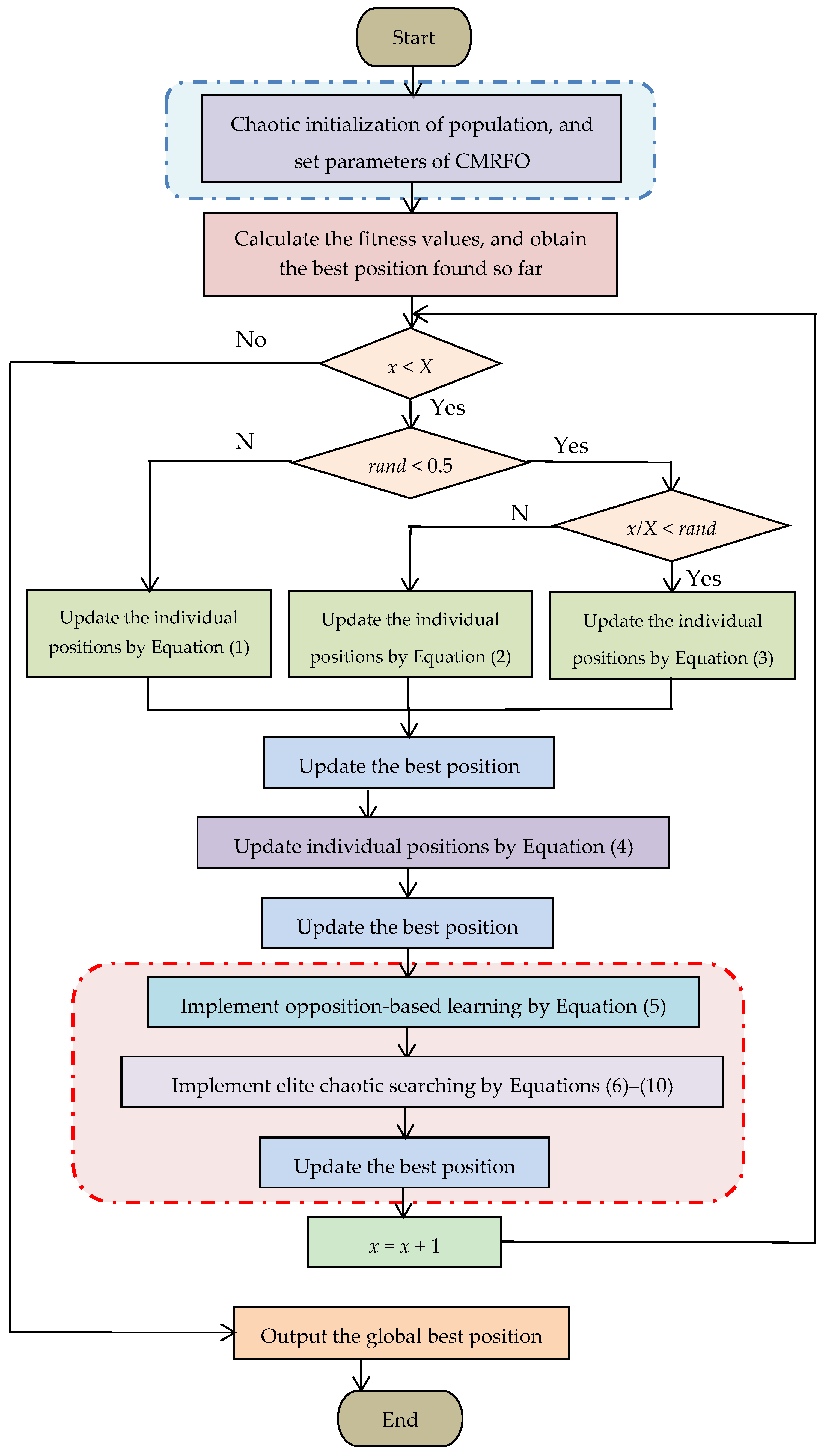
2. Proposed Chaotic MRFO
2.1. Overview of the MRFO
2.1.1. Chain Foraging (CF)
2.1.2. Spiral Foraging
2.1.3. Somersault Foraging (SF)
2.2. Chaotic MRFO
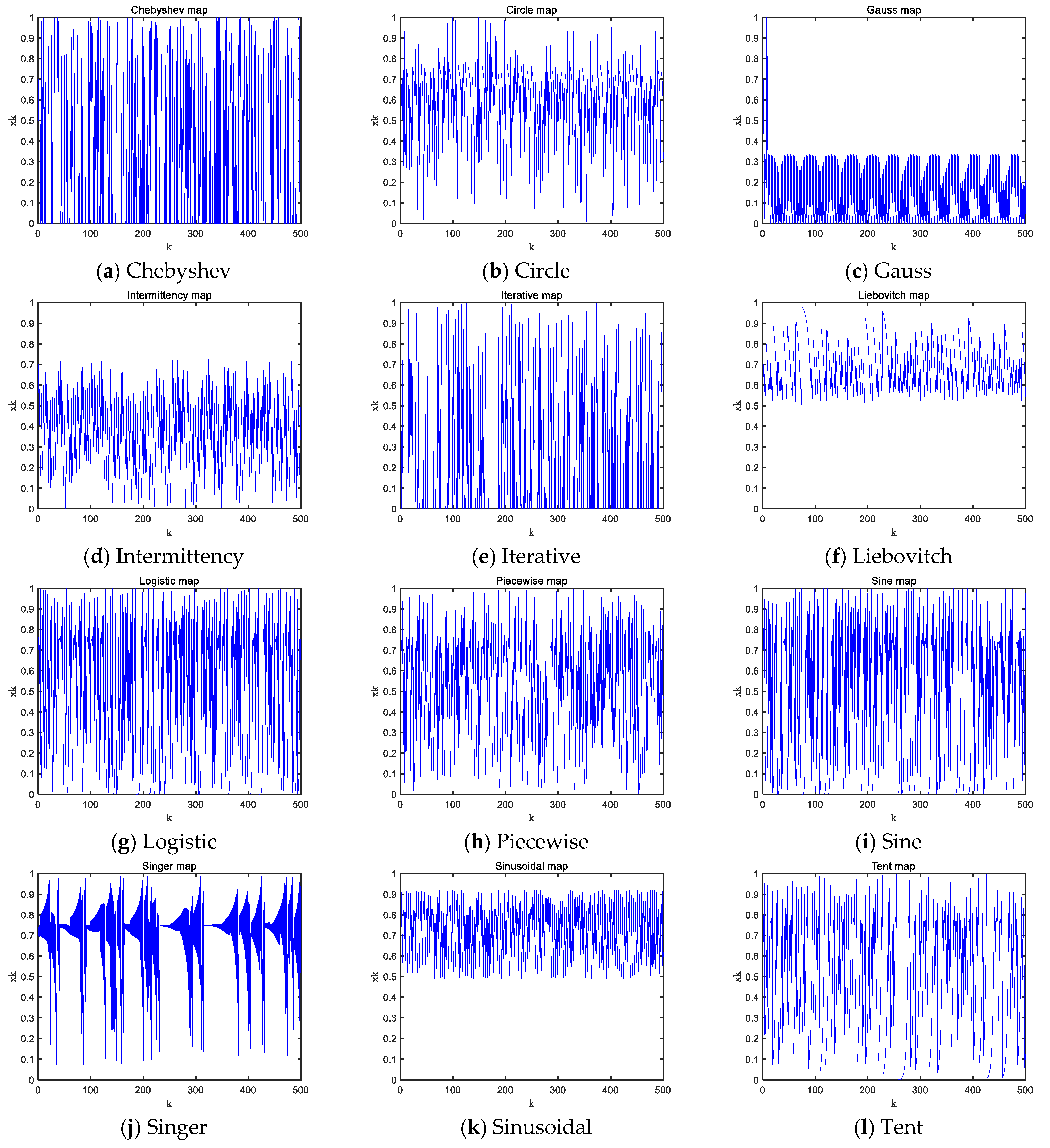
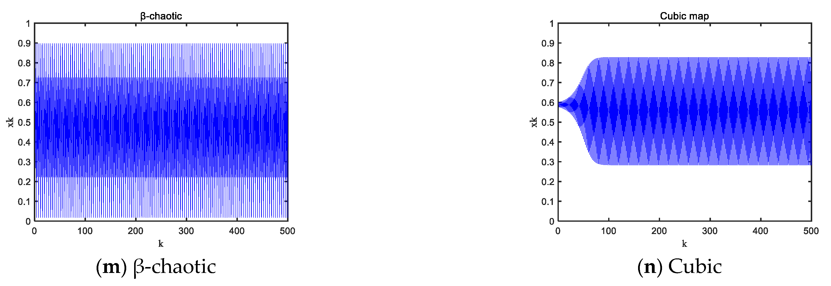
2.2.1. Chaotic Initialization of Population
2.2.2. Opposition-Based Learning (OL)
2.2.3. Elite Chaotic Searching (ECS)
| Algorithm 1: CMRFO |
| Set the parameters: M, X, Ub, Lb, D, p |
| The chaotic map is used to generate the initial position of N manta rays. //Chaotic initialization of population |
| Calculate the fitness value of each individual, and save the best position. |
| While x < X |
| for i = 1: M |
| for d = 1 to D |
| if rand < 0.5 //Cyclone foraging |
| if t/T < rand |
| else |
| end if |
| else //Chain foraging |
| end if |
| Update the best position. |
| //Somersault foraging |
| Update the best position. |
| //Opposition-based learning |
| The first N individuals among current and opposition-based individuals are selected as the new population. |
| The fitness values of the current population are sorted in ascending order, and the first n individuals are selected as elite individuals. //Elite chaotic searching |
| for I = 1 to n |
| for k = 1 to X |
| end for |
| if then |
| end if |
| end for |
| end for |
| end for |
| End while |
| Output the global best position. |

3. Experimental Results and Analysis
3.1. Performance of the CMRFO for the Initializing Population Based on Different Chaotic Maps
3.2. Elite Individual Proportion Analysis
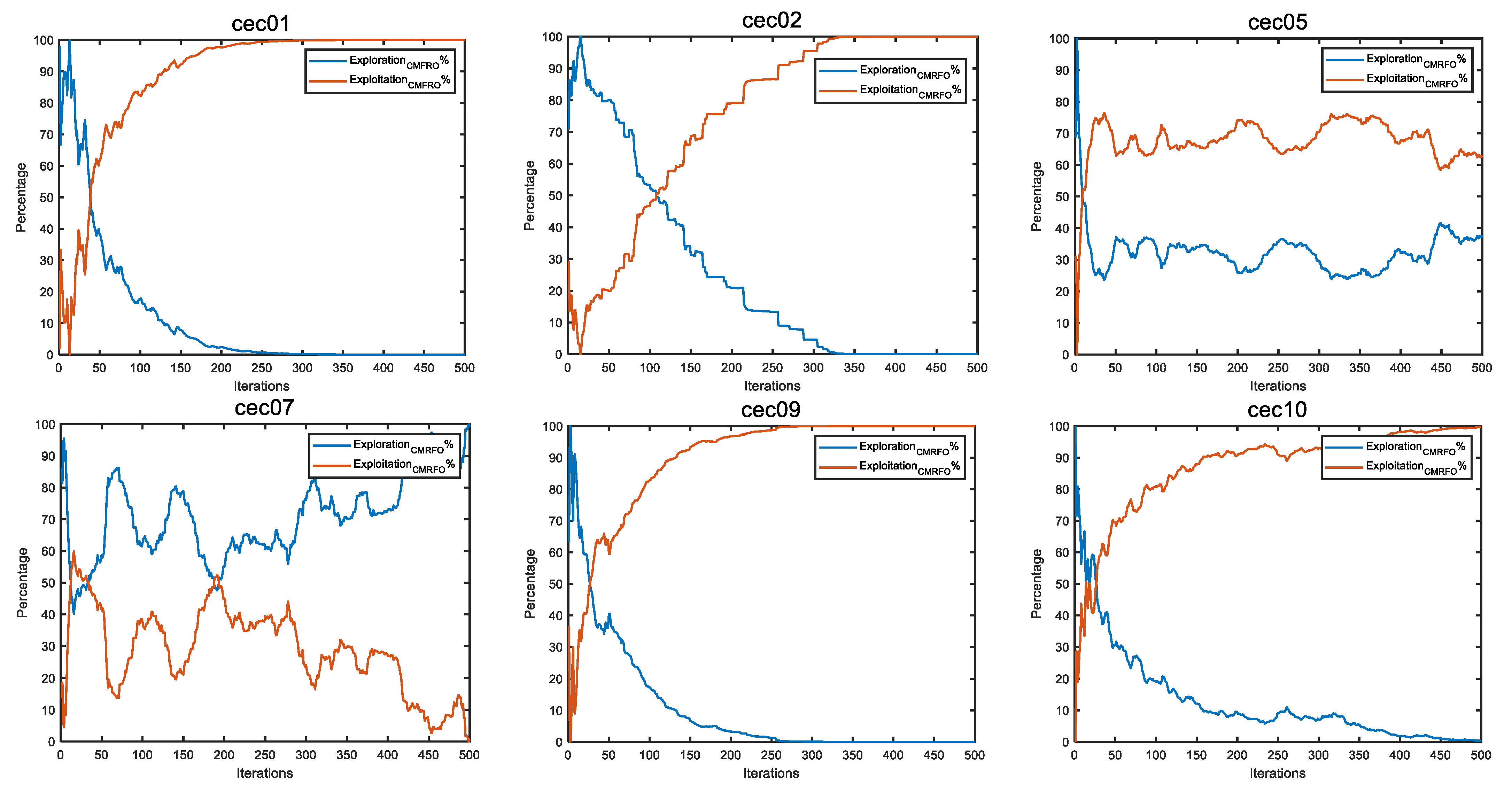
3.3. Exploration–Exploitation Analysis
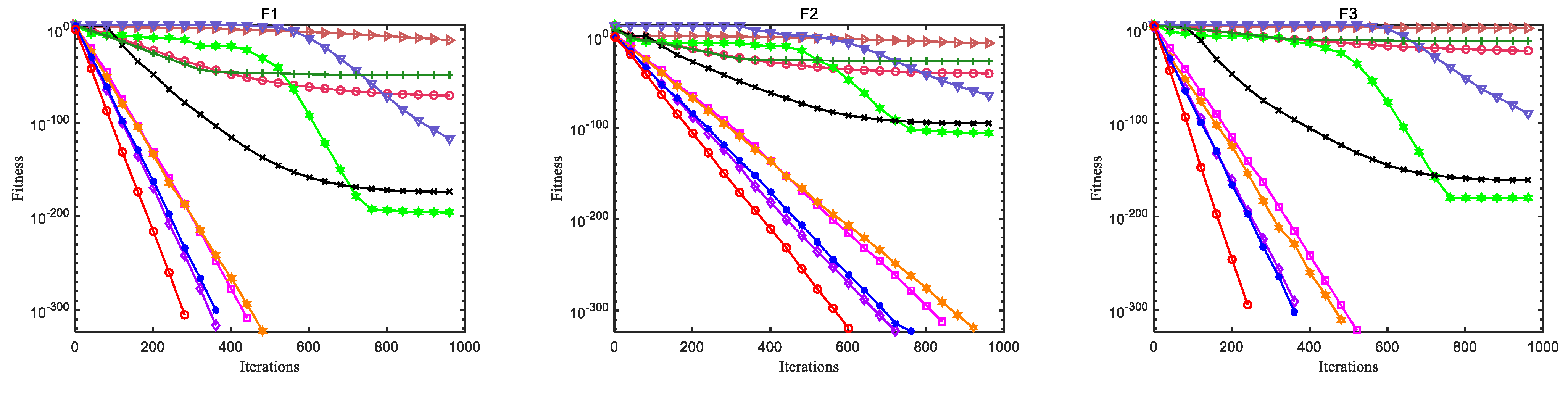
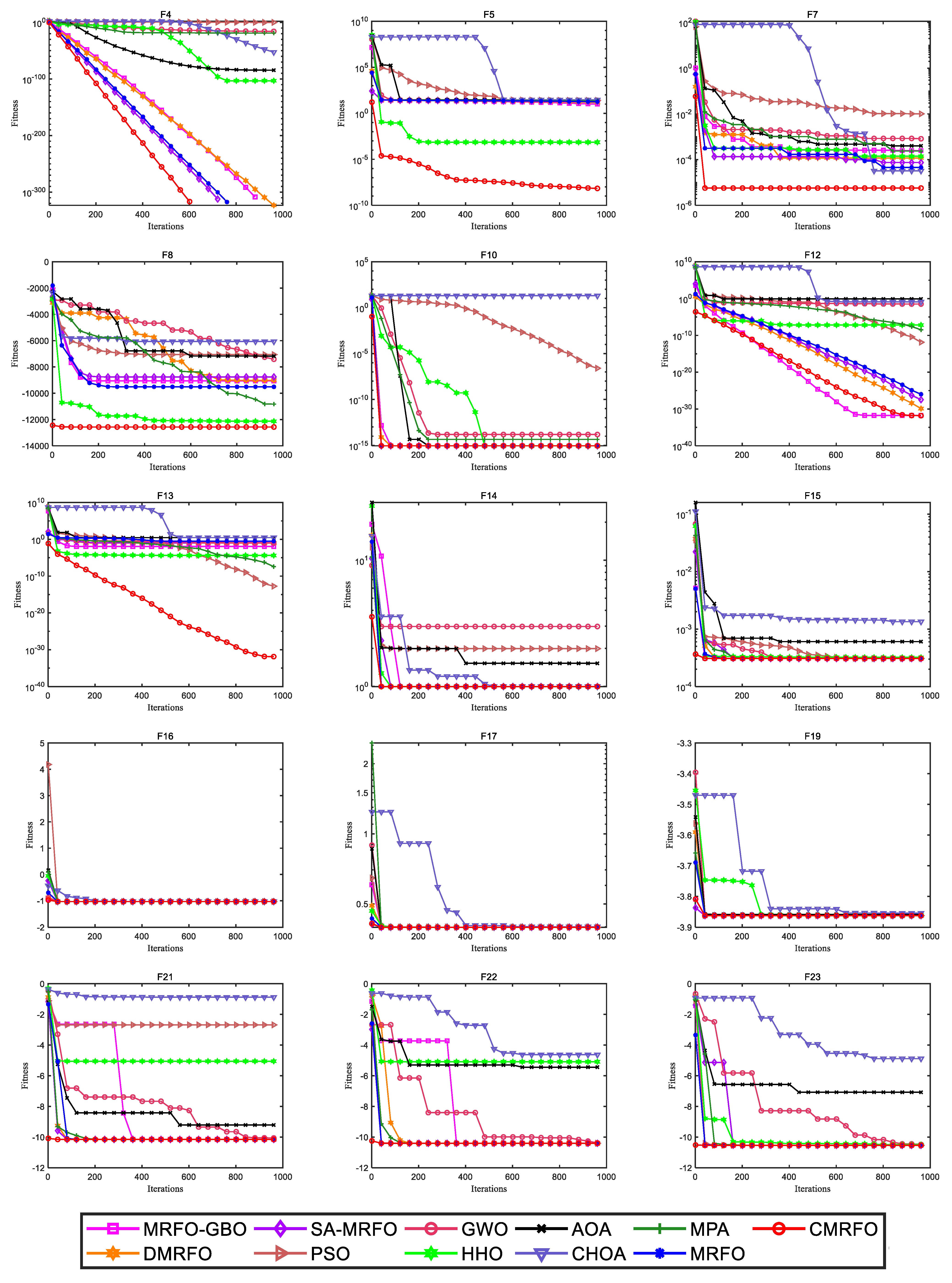
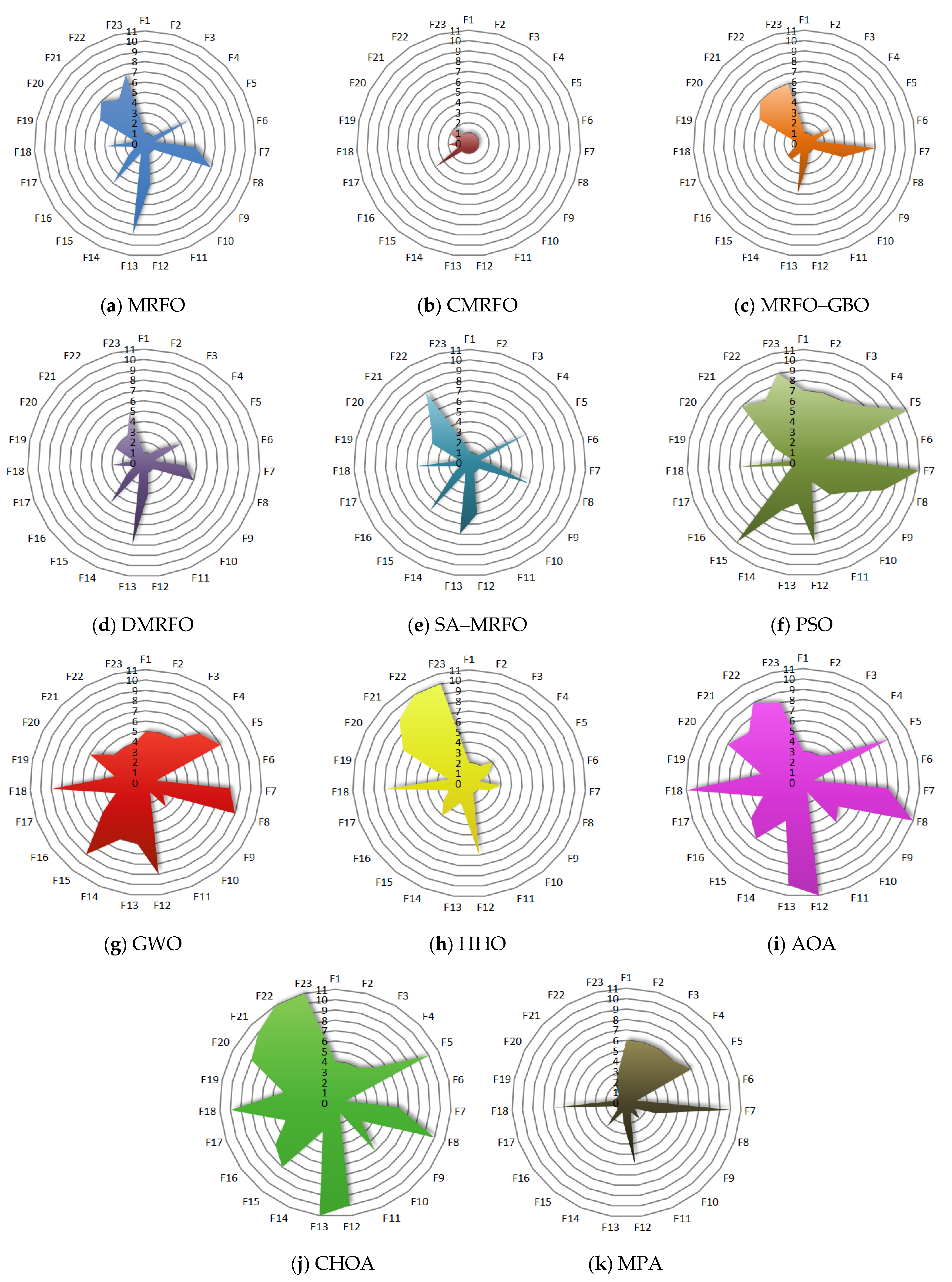
3.4. Comparison of the CMRFO with Other Optimizers on 23 Benchmark Functions
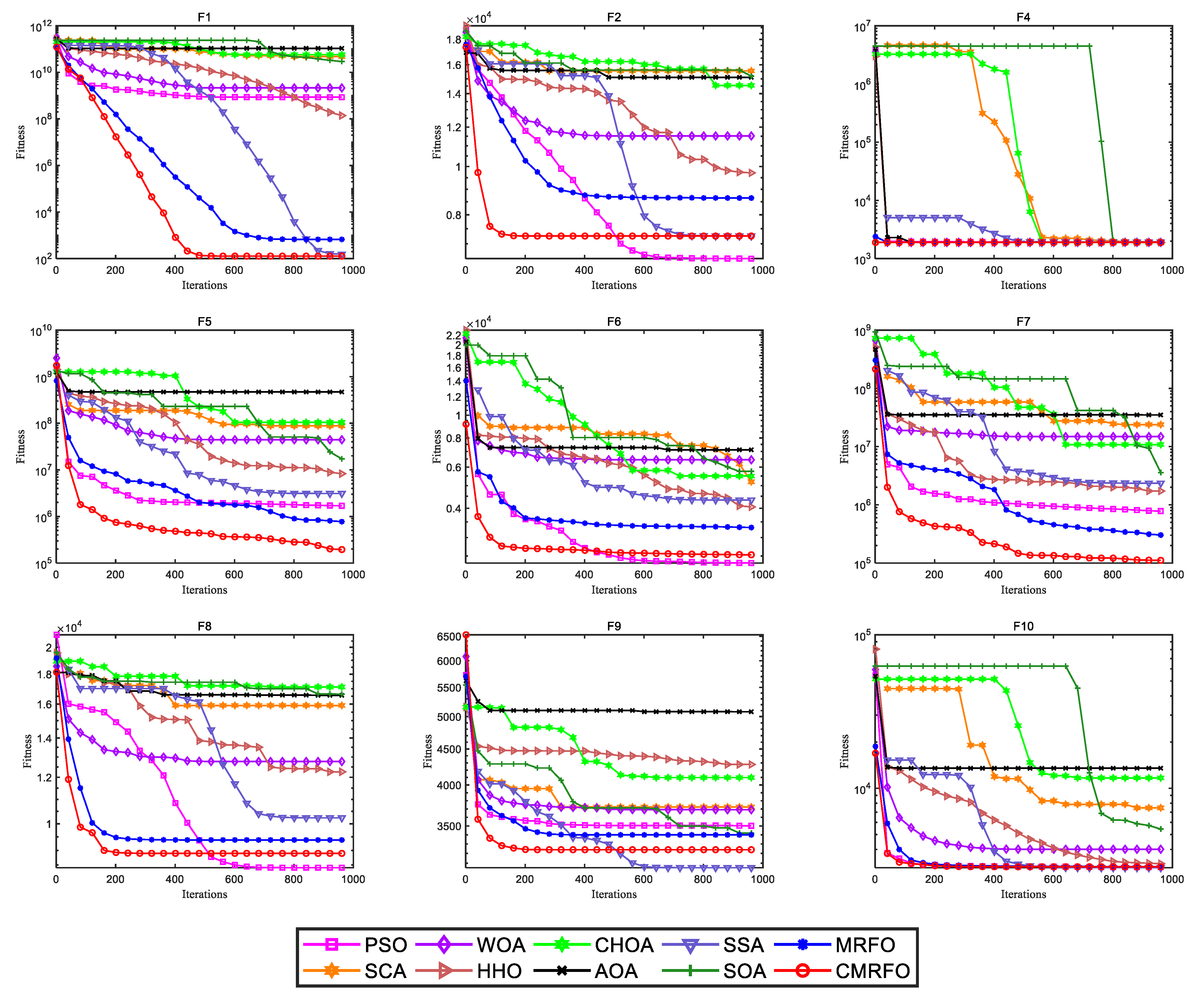
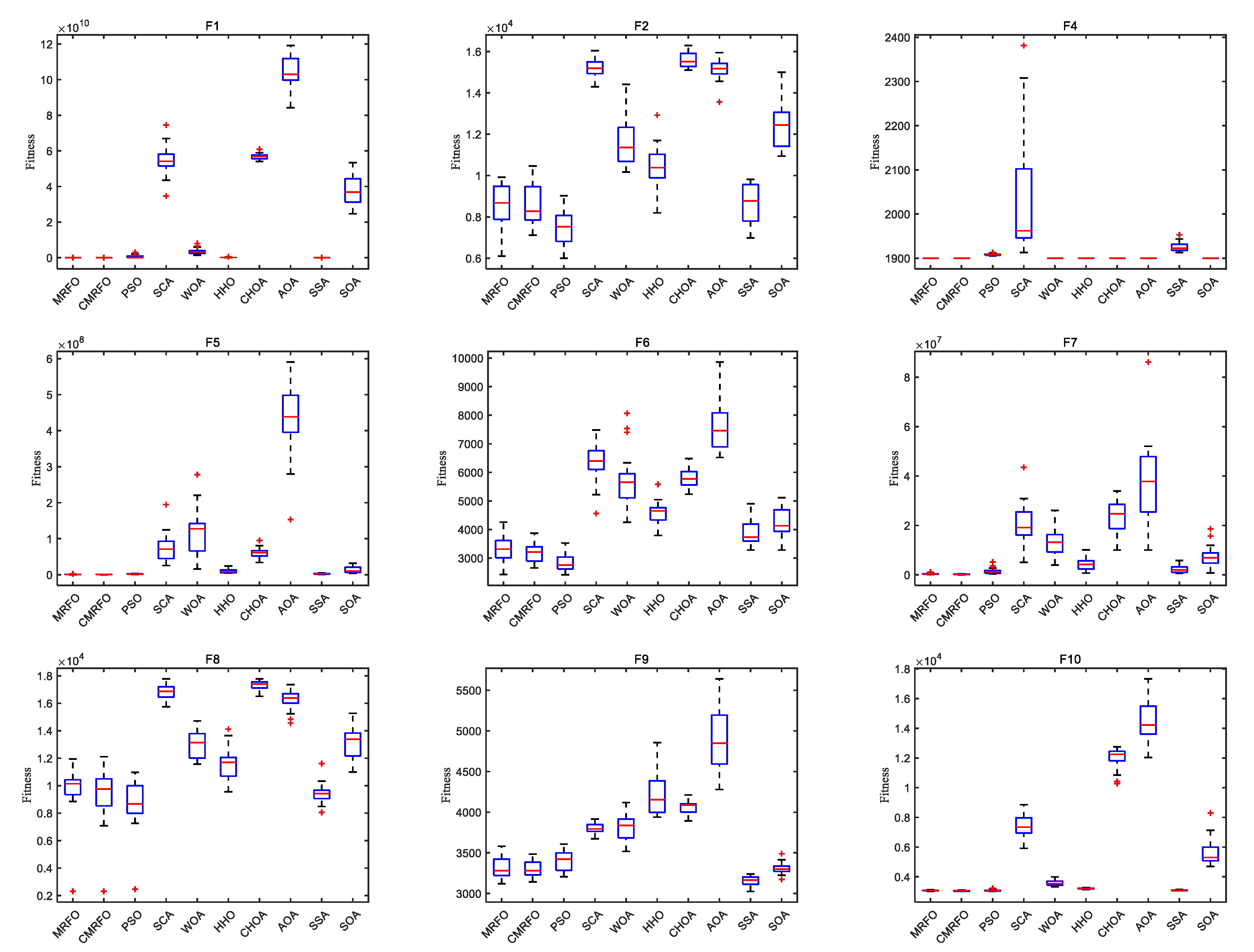
3.5. Comparison of the CMRFO with Other Optimizers on CEC2020
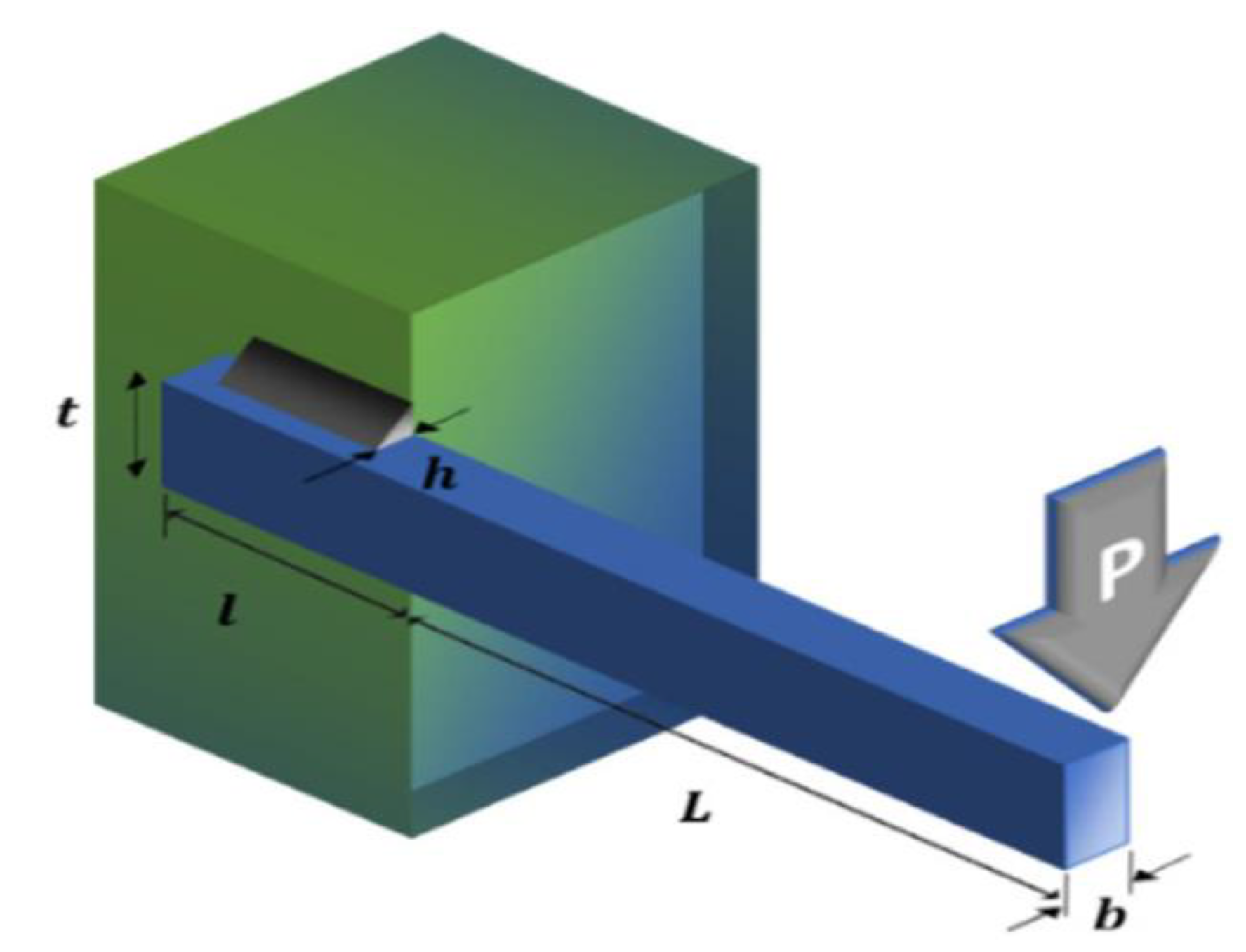
4. Practical Engineering Application
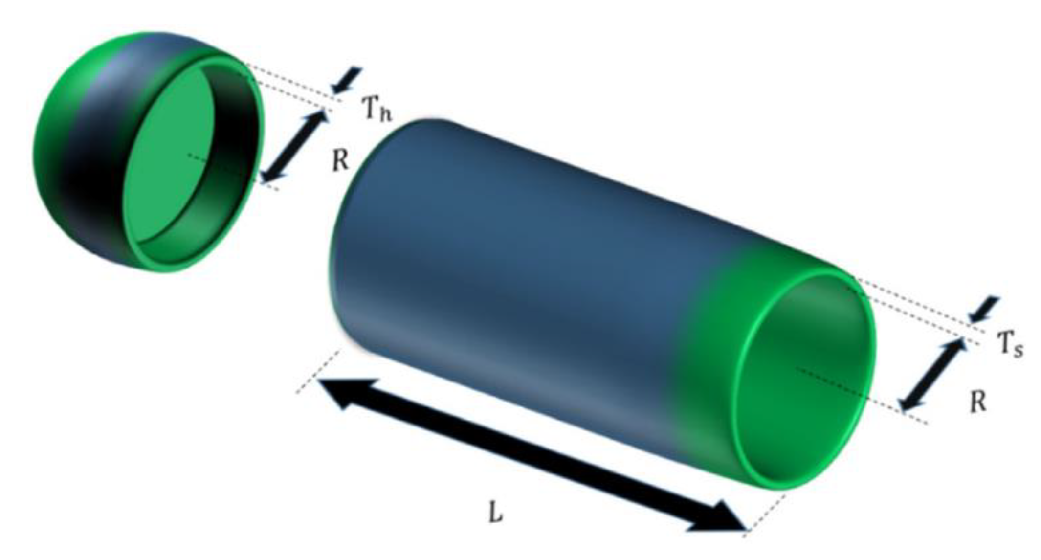
4.1. Pressure Vessel (PV) Design
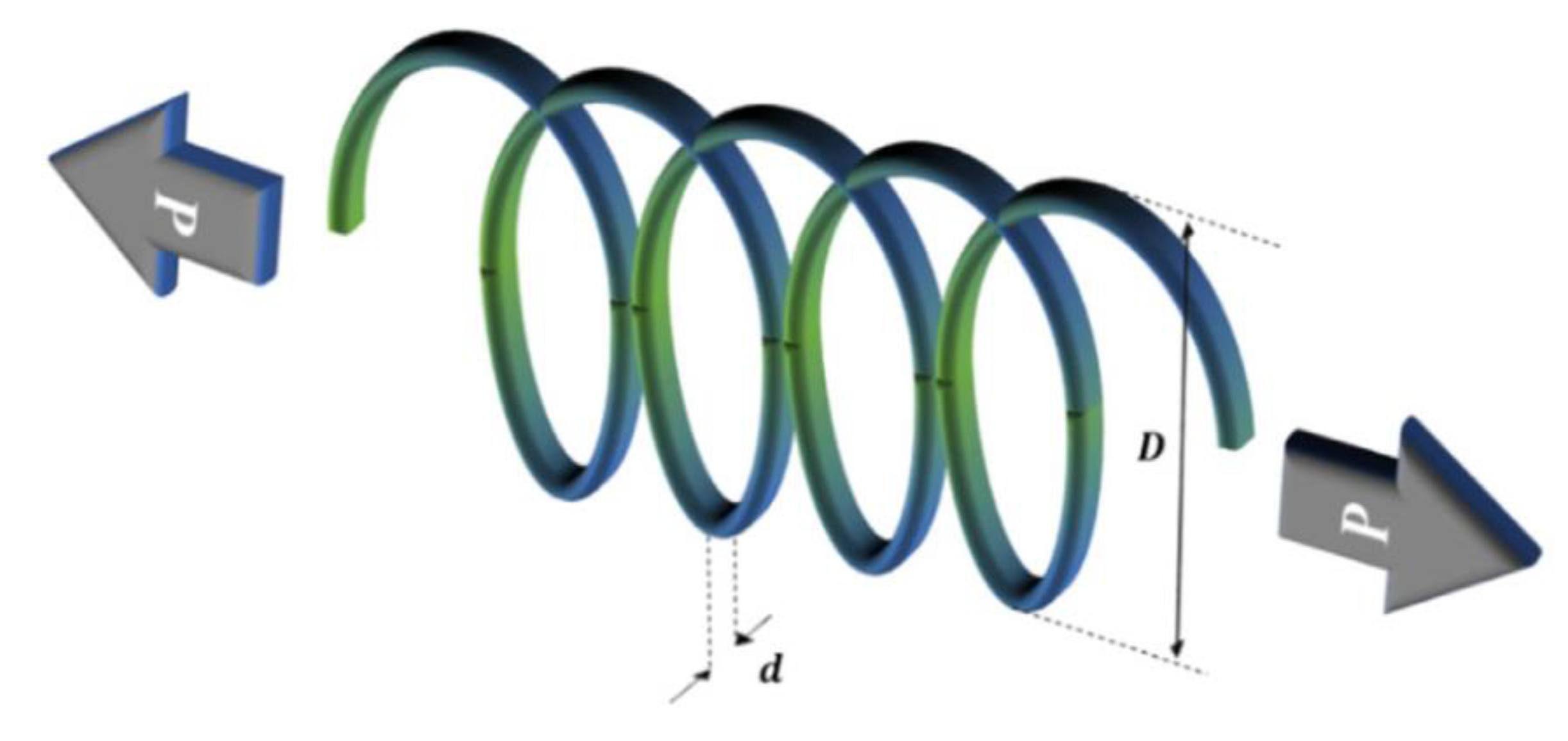
4.2. Tension/Compression Spring (TCS) Optimization Problem
4.3. Pressure Vessel (PV) Design
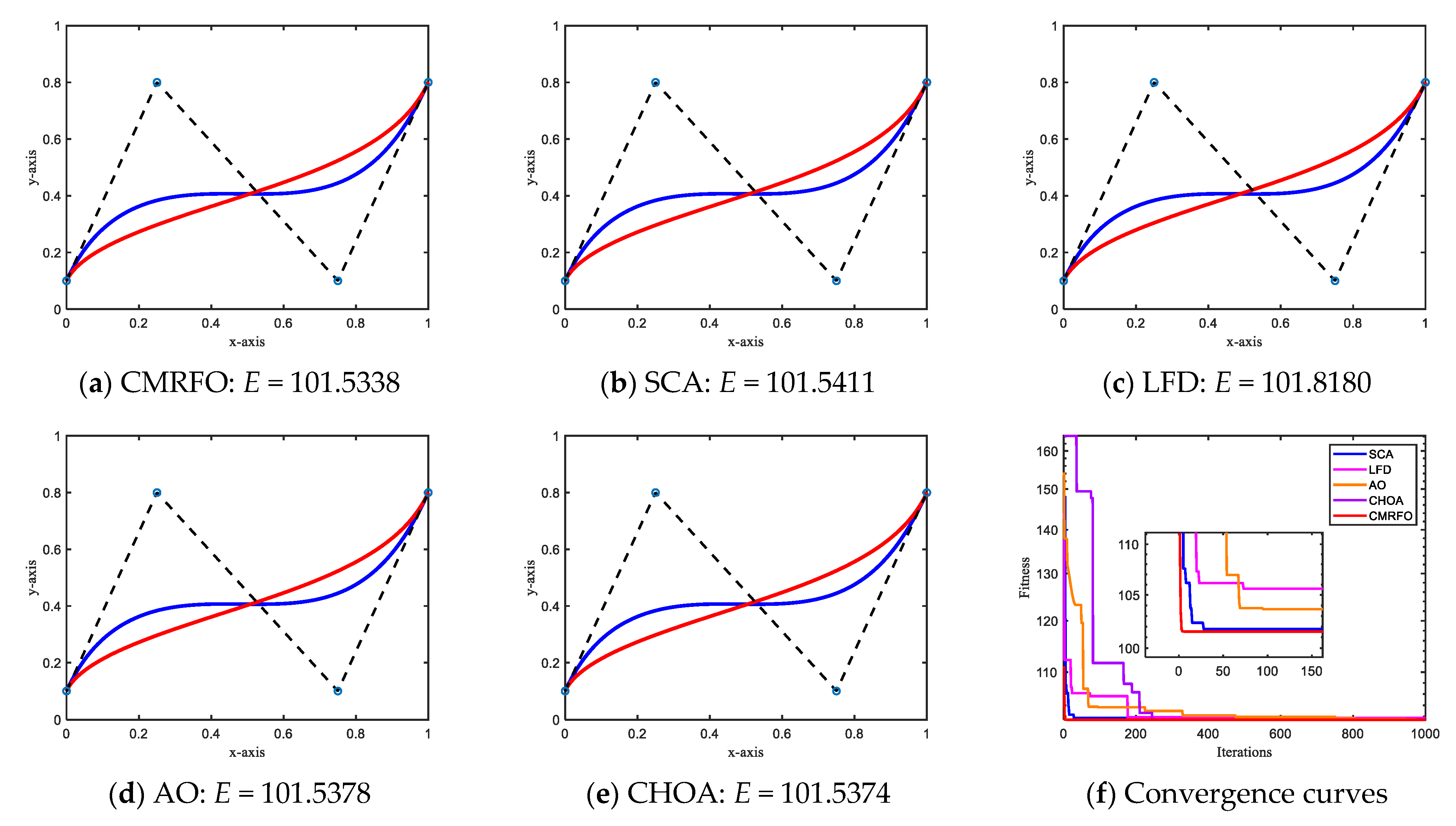
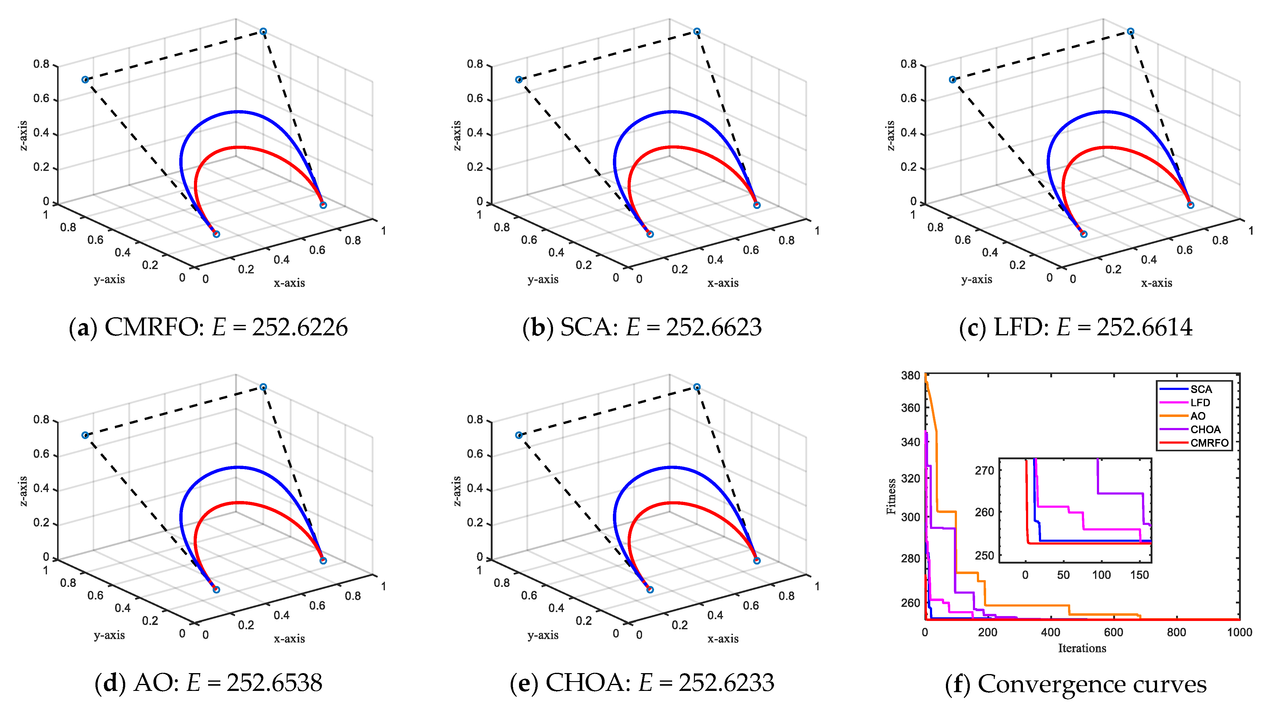
5. Real-World Application: Construction of CG-Ball Curves with Optimal Shape
5.1. Shape Optimization Model: Minimum Curvature Variation in Curves
| , | , |
| , | , |
| , | , |
| , | , |
| , | . |
5.2. Modeling Examples
6. Conclusions
Supplementary Materials
Author Contributions
Funding
Institutional Review Board Statement
Informed Consent Statement
Data Availability Statement
Acknowledgments
Conflicts of Interest
References
- Hackwood, S.; Beni, G. Self-organization of sensors for swarm intelligence. In Proceedings of the 1992 IEEE International Conference on Robotics and Automation, Nice, France, 12–14 May 1992; pp. 819–829. [Google Scholar]
- Holland, J.H. Genetic algorithms. Sci. Am. 1992, 267, 66–73. [Google Scholar] [CrossRef]
- Barshandeh, S.; Dana, R.; Eskandarian, P. A learning automata-based hybrid MPA and JS algorithm for numerical optimization problems and its application on data clustering. Knowl. Based Syst. 2021, 236, 107682. [Google Scholar] [CrossRef]
- Hu, G.; Du, B.; Wang, X.F.; Wei, G. An enhanced black widow optimization algorithm for feature selection. Knowl. Based Syst. 2022, 235, 107638. [Google Scholar] [CrossRef]
- Hassan, M.H.; Kamel, S.; Abualigah, L.; Eid, A. Development and application of slime mould algorithm for optimal economic emission dispatch. Expert Syst. Appl. 2021, 182, 115205. [Google Scholar] [CrossRef]
- Hu, G.; Zhong, J.; Du, B.; Wei, G. An enhanced hybrid arithmetic optimization algorithm for engineering applications. Comput. Methods Appl. Mech. Eng. 2022, 394, 114901. [Google Scholar] [CrossRef]
- Hu, G.; Zhu, X.N.; Wei, G.; Chang, C.T. An improved marine predators algorithm for shape optimization of developable Ball surfaces. Eng. Appl. Artif. Intell. 2021, 105, 104417. [Google Scholar] [CrossRef]
- Elsisi, M.; Ebrahim, M. Optimal design of low computational burden model predictive control based on SSDA towards autonomous vehicle under vision dynamics. Int. J. Intell. Syst. 2021, 36, 6968–6987. [Google Scholar] [CrossRef]
- Elsisi, M.; Ismail, M.; Bendary, A. Optimal design of battery charge management controller for hybrid system PV/wind cell with storage battery. Int. J. Power Energy Convers. 2020, 11, 412. [Google Scholar] [CrossRef]
- Elsisi, M.; Mahmoud, K.; Lehtonen, M.; Darwish, M.M.F. Effective Nonlinear Model Predictive Control Scheme Tuned by Improved NN for Robotic Manipulators. IEEE Access 2021, 9, 64278–64290. [Google Scholar] [CrossRef]
- Elsisi, M.; Soliman, M.; Aboelela, M.; Mansour, W. ABC based design of PID controller for two area load frequency control with nonlinearities. Telkomnika Indones. J. Electr. Eng. 2015, 16, 58–64. [Google Scholar] [CrossRef]
- Elsisi, M.; Tran, M.-Q.; Hasanien, H.M.; Turky, R.A.; Albalawi, F.; Ghoneim, S.S.M. Robust Model Predictive Control Paradigm for Automatic Voltage Regulators against Uncertainty Based on Optimization Algorithms. Mathematics 2021, 9, 2885. [Google Scholar] [CrossRef]
- Elsisi, M. Optimal design of nonlinear model predictive controller based on new modified multitracker optimization algorithm. Int. J. Intell. Syst. 2020, 35, 1857–1878. [Google Scholar] [CrossRef]
- Zheng, J.Y.; Hu, G.; Ji, X.; Qin, X. Quintic generalized Hermite interpolation curves: Construction and shape optimization using an improved GWO algorithm. Comput. Appl. Math. 2022, 41, 115. [Google Scholar] [CrossRef]
- Elsisi, M.; Abdelfattah, H. New design of variable structure control based on lightning search algorithm for nuclear reactor power system considering load-following operation. Nucl. Eng. Technol. 2020, 52, 544–551. [Google Scholar] [CrossRef]
- Hu, G.; Dou, W.; Wang, X.; Abbas, M. An enhanced chimp optimization algorithm for optimal degree reduction of Said–Ball curves. Math. Comput. Simul. 2022, 197, 207–252. [Google Scholar] [CrossRef]
- Zhao, W.; Zhang, Z.; Mirjalili, S.; Wang, L.; Khodadadi, N.; Mirjalili, S.M. An effective multi-objective artificial hummingbird algorithm with dynamic elimination-based crowding distance for solving engineering design problems. Comput. Methods Appl. Mech. Eng. 2022, 398, 115223. [Google Scholar] [CrossRef]
- Xie, Z.; Zhang, C.; Shao, X.; Lin, W.; Zhu, H. An effective hybrid teaching–learning-based optimization algorithm for permutation flow shop scheduling problem. Adv. Eng. Softw. 2014, 77, 35–47. [Google Scholar] [CrossRef]
- Hu, G.; Li, M.; Wang, X.; Wei, G.; Chang, C.-T. An enhanced manta ray foraging optimization algorithm for shape optimization of complex CCG-Ball curves. Knowl. Based Syst. 2022, 240, 108071. [Google Scholar] [CrossRef]
- Elsisi, M. Improved grey wolf optimizer based on opposition and quasi learning approaches for optimization: Case study autonomous vehicle including vision system. Artif. Intell. Rev. 2022, 1–24. [Google Scholar] [CrossRef]
- Hu, G.; Du, B.; Li, H.N.; Wang, X.P. Quadratic interpolation boosted black widow spider-inspired optimization algorithm with wavelet mutation. Math. Comput. Simul. 2022, 200, 428–467. [Google Scholar] [CrossRef]
- Zhao, W.; Shi, T.; Wang, L.; Cao, Q.; Zhang, H. An adaptive hybrid atom search optimization with particle swarm optimization and its application to optimal no-load PID design of hydro-turbine governor. J. Comput. Des. Eng. 2021, 8, 1204–1233. [Google Scholar] [CrossRef]
- Zhao, W.G.; Zhang, Z.X.; Wang, L.Y. Manta ray foraging optimization: An effective bio-inspired optimizer for engineering applications. Eng. Appl. Artif. Intell. 2020, 87, 103300. [Google Scholar] [CrossRef]
- Houssein, E.H.; Zaki, G.N.; Diab, A.A.Z.; Younis, E.M.G. An efficient manta ray foraging optimization algorithm for parameter extraction of three-diode photovoltaic model. Comput. Electr. Eng. 2021, 94, 107304. [Google Scholar] [CrossRef]
- Fathy, A.; Rezk, H.; Yousri, D. A robust global MPPT to mitigate partial shading of triple-junction solar cell-based system using manta ray foraging optimization algorithm. Sol. Energy 2020, 207, 305–316. [Google Scholar] [CrossRef]
- Ben, U.C.; Akpan, A.E.; Enyinyi, E.O.; Awak, E. Novel technique for the interpretation of gravity anomalies over geologic structures with idealized geometries using the manta ray foraging optimization. J. Asian Earth Sci. X 2021, 6, 100070. [Google Scholar] [CrossRef]
- Ben, U.C.; Akpan, A.E.; Mbonu, C.C.; Ebong, E.D. Novel methodology for interpretation of magnetic anomalies due to two-dimensional dipping dikes using the manta ray foraging optimization. J. Appl. Geophys. 2021, 192, 104405. [Google Scholar] [CrossRef]
- El-Hameed, M.A.; Elkholy, M.M.; El-Fergany, A.A. Three-diode model for characterization of industrial solar generating units using manta-rays foraging optimizer: Analysis and validations. Energy Convers. Manag. 2020, 219, 113048. [Google Scholar] [CrossRef]
- Houssein, E.H.; Ibrahim, I.E.; Neggaz, N.; Hassaballah, M.; Wazery, Y.M. An efficient ECG arrhythmia classification method based on manta ray foraging optimization. Expert Syst. Appl. 2021, 181, 115131. [Google Scholar] [CrossRef]
- Hemeida, M.G.; Ibrahim, A.A.; Mohamed, A.A.; Alkhalaf, S.; El-Dine, A.M.B. Optimal allocation of distributed generators DG based manta ray foraging optimization algorithm (MRFO). Ain Shams Eng. J. 2021, 12, 609–619. [Google Scholar] [CrossRef]
- Elmaadawy, K.; Elaziz, M.A.; Elsheikh, A.H.; Moawad, A.; Liu, B.C.; Lu, S.F. Utilization of random vector functional link integrated with manta ray foraging optimization for effluent prediction of wastewater treatment plant. J. Environ. Manag. 2021, 298, 113520. [Google Scholar] [CrossRef]
- Got, A.; Zouache, D.; Moussaoui, A. MOMRFO: Multi-objective manta ray foraging optimizer for handling engineering design problems. Knowl. Based Syst. 2022, 237, 107880. [Google Scholar] [CrossRef]
- Zouache, D.; Abdelaziz, F.B. Guided manta ray foraging optimization using epsilon dominance for multi-objective optimization in engineering design. Expert Syst. Appl. 2022, 189, 116126. [Google Scholar] [CrossRef]
- Kahraman, H.T.; Akbel, M.; Duman, S. Optimization of optimal power flow problem using multi-objective manta ray foraging optimizer. Appl. Soft Comput. 2022, 116, 108334. [Google Scholar] [CrossRef]
- Elaziz, M.A.; Yousri, D.; Al-Qaness, M.A.A.; AbdelAty, A.M.; Radwan, A.G.; Ewees, A.A. A Grunwald–Letnikov based manta ray foraging optimizer for global optimization and image segmentation. Eng. Appl. Artif. Intell. 2021, 98, 104105. [Google Scholar] [CrossRef]
- Hu, S.M.; Wang, G.Z.; Jin, T.G. Properties of two types of generalized Ball curves. Comput. Aided Des. 1996, 28, 125–133. [Google Scholar] [CrossRef]
- Yousri, D.; AbdelAty, A.M.; Al-qaness, M.A.A.; Ewees, A.A.; Radwan, A.G.; Elaziz, M.A. Discrete fractional-order Caputo method to overcome trapping in local optima: Manta ray foraging optimizer as a case study. Expert Syst. Appl. 2022, 192, 116355. [Google Scholar] [CrossRef]
- Xu, H.T.; Song, H.Q.; Xu, C.X.; Wu, X.W.; Yousefi, N. Exergy analysis and optimization of a HT-PEMFC using developed manta ray foraging optimization algorithm. Int. J. Hydrog. Energy 2020, 45, 30932–30941. [Google Scholar] [CrossRef]
- Jena, B.; Naik, M.K.; Panda, R.; Abraham, A. Maximum 3D Tsallis entropy based multilevel thresholding of brain MR image using attacking manta ray foraging optimization. Eng. Appl. Artif. Intell. 2021, 103, 104293. [Google Scholar] [CrossRef]
- Feng, J.Y.; Luo, X.G.; Gao, M.Z.; Abbas, A.; Xu, Y.P.; Pouramini, S. Minimization of energy consumption by building shape optimization using an improved manta-ray foraging optimization algorithm. Energy Rep. 2021, 7, 1068–1078. [Google Scholar] [CrossRef]
- Liu, B.Z.; Wang, Z.Z.; Feng, L.; Jermsittiparsert, K. Optimal operation of photovoltaic/diesel generator/pumped water reservoir power system using modified manta ray optimization. J. Clean. Prod. 2021, 289, 125733. [Google Scholar] [CrossRef]
- Sheng, B.Q.; Pan, T.H.; Luo, Y.; Jermsittiparsert, K. System identification of the PEMFCs based on balanced manta-ray foraging optimization algorithm. Energy Rep. 2020, 6, 2887–2896. [Google Scholar] [CrossRef]
- Micev, M.; Ćalasan, M.; Ali, Z.M.; Hasanien, H.M.; Aleem, S.H.E.A. Optimal design of automatic voltage regulation controller using hybrid simulated annealing—Manta ray foraging optimization algorithm. Ain Shams Eng. J. 2021, 12, 641–657. [Google Scholar] [CrossRef]
- Hassan, M.H.; Houssein, E.H.; Mahdy, M.A.; Kamel, S. An improved manta ray foraging optimizer for cost-effective emission dispatch problems. Eng. Appl. Artif. Intell. 2021, 100, 104155. [Google Scholar] [CrossRef]
- Jain, S.; Indora, S.; Atal, D.K. Rider manta ray foraging optimization-based generative adversarial network and CNN feature for detecting glaucoma, Biomed. Signal Process. Control 2022, 73, 103425. [Google Scholar] [CrossRef]
- Kennedy, J.; Eberhart, R. Particle swarm optimization. In Proceedings of the 1995 IEEE International Conference on Neural Networks, Perth, WA, Australia, 27 November–1 December 1995; pp. 1942–1948. [Google Scholar]
- Mirjalili, S.; Mirjalili, S.M.; Lewis, A. Grey wolf optimizer. Adv. Eng. Softw. 2014, 69, 46–61. [Google Scholar] [CrossRef]
- Heidari, A.A.; Mirjalili, S.; Faris, H.; Aljarah, I.; Mafarja, M.; Chen, H.L. Harris hawks optimization: Algorithm and applications. Future Gener. Comput. Syst. 2019, 97, 849–872. [Google Scholar] [CrossRef]
- Hashim, F.A.; Hussain, K.; Houssein, E.H.; Mabrouk, M.S.; Al-Atabany, W. Archimedes optimization algorithm: A new metaheuristic algorithm for solving optimization problems. Appl. Intell. 2021, 51, 1531–1551. [Google Scholar] [CrossRef]
- Khishe, M.; Mosavi, M.R. Chimp optimization algorithm. Expert Syst. Appl. 2020, 149, 113338. [Google Scholar] [CrossRef]
- Faramarzi, A.; Heidarinejad, M.; Mirjalili, S.; Gandomi, A.H. Marine predators algorithm: A nature-inspired metaheuristic. Expert Syst. Appl. 2020, 152, 113377. [Google Scholar] [CrossRef]
- Mirjalili, S. SCA: A sine cosine algorithm for solving optimization problems. Knowl. Based Syst. 2016, 96, 120–133. [Google Scholar] [CrossRef]
- Mirjalili, S.; Lewis, A. The whale optimization algorithm. Adv. Eng. Softw. 2016, 95, 51–67. [Google Scholar] [CrossRef]
- Mirjalili, S.; Gandomi, A.H.; Mirjalili, S.Z.; Saremi, S.; Faris, H.; Mirjalili, S.M. Salp swarm algorithm: A bio-inspired optimizer for engineering design problems. Adv. Eng. Softw. 2017, 114, 163–191. [Google Scholar] [CrossRef]
- Dhiman, G.; Kumar, V. Seagull optimization algorithm: Theory and its applications for large-scale industrial engineering problems. Knowl. Based Syst. 2019, 165, 169–196. [Google Scholar] [CrossRef]
- Abualigah, L.; Yousri, D.; Elaziz, M.A.; Ewees, A.A.; Al-qaness, M.A.A.; Gandomi, A.H. Aquila optimizer: A novel meta-heuristic optimization algorithm. Comput. Ind. Eng. 2021, 157, 107250. [Google Scholar] [CrossRef]
- Kaur, S.; Awasthi, L.K.; Sangal, A.L.; Dhiman, G. Tunicate swarm algorithm: A new bio-inspired based metaheuristic paradigm for global optimization. Eng. Appl. Artif. Intell. 2020, 90, 103541. [Google Scholar] [CrossRef]
- Chou, J.S.; Truong, D.N. A novel metaheuristic optimizer inspired by behavior of jellyfish in ocean. Appl. Math. Comput. 2021, 389, 125535. [Google Scholar] [CrossRef]
- Houssein, E.H.; Saad, M.R.; Hashim, F.A.; Shaban, H.; Hassaballah, M. Lévy flight distribution: A new metaheuristic algorithm for solving engineering optimization problems. Eng. Appl. Artif. Intell. 2020, 94, 103731. [Google Scholar] [CrossRef]


| No. | Map Name | Map Equation |
|---|---|---|
| 1 | Chebyshev (M1) | |
| 2 | Circle (M2) | |
| 3 | Gauss/mouse (M3) | |
| 4 | Intermittency (M4) | |
| 5 | Iterative (M5) | |
| 6 | Liebovitch (M6) | |
| 7 | Logistic (M7) | |
| 8 | Piecewise (M8) | |
| 9 | Sine (M9) | |
| 10 | Singer (M10) | |
| 11 | Sinusoidal (M11) | |
| 12 | Tent (M12) | |
| 13 | β-chaotic (M13) | |
| 14 | Cubic (M14) |
| No. | Result | CMRFO | ||||||
|---|---|---|---|---|---|---|---|---|
| M1 | M2 | M3 | M4 | M5 | M6 | M7 | ||
| F1 | Mean | 0.0 | 0.0 | 0.0 | 0.0 | 0.0 | 0.0 | 0.0 |
| Std | 0.0 | 0.0 | 0.0 | 0.0 | 0.0 | 0.0 | 0.0 | |
| Rank | 1.0 | 1.0 | 1.0 | 1.0 | 1.0 | 1.0 | 1.0 | |
| F2 | Mean | 0.0 | 0.0 | 0.0 | 0.0 | 0.0 | 0.0 | 0.0 |
| Std | 0.0 | 0.0 | 0.0 | 0.0 | 0.0 | 0.0 | 0.0 | |
| Rank | 1.0 | 1.0 | 1.0 | 1.0 | 1.0 | 1.0 | 1.0 | |
| F3 | Mean | 0.0 | 0.0 | 0.0 | 0.0 | 0.0 | 0.0 | 0.0 |
| Std | 0.0 | 0.0 | 0.0 | 0.0 | 0.0 | 0.0 | 0.0 | |
| Rank | 1.0 | 1.0 | 1.0 | 1.0 | 1.0 | 1.0 | 1.0 | |
| F4 | Mean | 0.0 | 0.0 | 0.0 | 0.0 | 0.0 | 0.0 | 0.0 |
| Std | 0.0 | 0.0 | 0.0 | 0.0 | 0.0 | 0.0 | 0.0 | |
| Rank | 1.0 | 1.0 | 1.0 | 1.0 | 1.0 | 1.0 | 1.0 | |
| F5 | Mean | 8.70060 | 0.90144 | 1.76270 | 2.17 × 10⁻⁷ | 7.80430 | 0.89795 | 0.88399 |
| Std | 79.7595 | 16.2520 | 29.5025 | 8.89 × 10⁻¹³ | 78.6172 | 16.1263 | 15.6288 | |
| Rank | 14 | 7 | 11 | 3 | 13 | 6 | 5 | |
| F6 | Mean | 0.0 | 0.0 | 0.0 | 0.0 | 0.0 | 0.0 | 0.0 |
| Std | 0.0 | 0.0 | 0.0 | 0.0 | 0.0 | 0.0 | 0.0 | |
| Rank | 1.0 | 1.0 | 1.0 | 1.0 | 1.0 | 1.0 | 1.0 | |
| F7 | Mean | 3.26 × 10⁻⁵ | 5.28 × 10⁻⁵ | 4.33 × 10⁻⁵ | 4.65 × 10⁻⁵ | 5.44 × 10⁻⁵ | 4.37 × 10⁻⁵ | 3.88 × 10⁻⁵ |
| Std | 4.58 × 10⁻¹⁰ | 1.29 × 10⁻⁹ | 1.20 × 10⁻⁹ | 1.71 × 10⁻⁹ | 1.63 × 10⁻⁹ | 1.87 × 10⁻⁹ | 7.27 × 10⁻¹⁰ | |
| Rank | 1 | 12 | 6 | 8 | 13 | 7 | 3 | |
| F8 | Mean | −38,051.19 | −12,569.49 | −12,391.83 | −9584.84 | −39,165.73 | −12,569.49 | −12,569.49 |
| Std | 0.0 | 2.35 × 10⁻²³ | 6.31 × 10⁵ | 1.66 × 10⁶ | 5.57 × 10⁻²³ | 1.41 × 10⁻²³ | 1.60 × 10⁻²³ | |
| Rank | 13 | 10 | 11 | 12 | 14 | 5 | 7 | |
| F9 | Mean | 0.0 | 0.0 | 0.0 | 0.0 | 0.0 | 0.0 | 0.0 |
| Std | 0.0 | 0.0 | 0.0 | 0.0 | 0.0 | 0.0 | 0.0 | |
| Rank | 1.0 | 1.0 | 1.0 | 1.0 | 1.0 | 1.0 | 1.0 | |
| F10 | Mean | 8.88 × 10⁻¹⁶ | 8.88 × 10⁻¹⁶ | 8.88 × 10⁻¹⁶ | 8.88 × 10⁻¹⁶ | 8.88 × 10⁻¹⁶ | 8.88 × 10⁻¹⁶ | 8.88 × 10⁻¹⁶ |
| Std | 0.0 | 0.0 | 0.0 | 0.0 | 0.0 | 0.0 | 0.0 | |
| Rank | 1.0 | 1.0 | 1.0 | 1.0 | 1.0 | 1.0 | 1.0 | |
| F11 | Mean | 0.0 | 0.0 | 0.0 | 0.0 | 0.0 | 0.0 | 0.0 |
| Std | 0.0 | 0.0 | 0.0 | 0.0 | 0.0 | 0.0 | 0.0 | |
| Rank | 1.0 | 1.0 | 1.0 | 1.0 | 1.0 | 1.0 | 1.0 | |
| F12 | Mean | 1.88 × 10⁻³⁰ | 1.04 × 10⁻³¹ | 3.61 × 10⁻³¹ | 9.12 × 10⁻³² | 2.06 × 10⁻³⁰ | 8.87 × 10⁻³² | 2.68 × 10⁻³¹ |
| Std | 2.61 × 10−59 | 5.64 × 10−62 | 2.93 × 10−61 | 6.34 × 10−62 | 2.56 × 10−59 | 2.65 × 10−62 | 7.27 × 10−61 | |
| Rank | 13 | 5 | 11 | 4 | 14 | 3 | 9 | |
| F13 | Mean | 1.38 × 10⁻²⁹ | 7.61 × 10⁻³¹ | 1.15 × 10⁻²⁹ | 1.87 × 10⁻³¹ | 5.49 × 10⁻⁴ | 2.35 × 10⁻³¹ | 5.92 × 10⁻³¹ |
| Std | 1.08 × 10−57 | 3.98 × 10−60 | 3.90 × 10−58 | 1.77 × 10−61 | 6.04 × 10⁻⁶ | 7.95 × 10−62 | 1.46 × 10−60 | |
| Rank | 13 | 7 | 12 | 2 | 14 | 3 | 6 | |
| F14 | Mean | 0.998 | 0.998 | 0.998 | 0.998 | 0.998 | 0.998 | 0.998 |
| Std | 0.0 | 0.0 | 0.0 | 0.0 | 0.0 | 0.0 | 0.0 | |
| Rank | 1.0 | 1.0 | 1.0 | 1.0 | 1.0 | 1.0 | 1.0 | |
| F15 | Mean | 3.53 × 10⁻⁴ | 3.07 × 10⁻⁴ | 3.53 × 10⁻⁴ | 3.07 × 10⁻⁴ | 3.53 × 10⁻⁴ | 3.07 × 10⁻⁴ | 3.07 × 10⁻⁴ |
| Std | 4.19 × 10⁻⁸ | 5.88 × 10−38 | 4.19 × 10⁻⁸ | 3.37 × 10−38 | 4.19 × 10⁻⁸ | 2.68 × 10−38 | 2.26 × 10−38 | |
| Rank | 11 | 10 | 11 | 9 | 11 | 3 | 2 | |
| F16 | Mean | −1.0316 | −1.0316 | −1.0316 | −1.0316 | −1.0316 | −1.0316 | −1.0316 |
| Std | 5.19 × 10⁻³² | 5.19 × 10⁻³² | 5.19 × 10⁻³² | 5.19 × 10⁻³² | 5.19 × 10⁻³² | 5.19 × 10⁻³² | 5.19 × 10⁻³² | |
| Rank | 1.0 | 1.0 | 1.0 | 1.0 | 1.0 | 1.0 | 1.0 | |
| F17 | Mean | 0.39789 | 0.39789 | 0.39789 | 0.39789 | 0.39789 | 0.39789 | 0.39789 |
| Std | 0.0 | 0.0 | 0.0 | 0.0 | 0.0 | 0.0 | 0.0 | |
| Rank | 1.0 | 1.0 | 1.0 | 1.0 | 1.0 | 1.0 | 1.0 | |
| F18 | Mean | 3 | 3 | 3 | 3 | 3 | 3 | 3 |
| Std | 4.05 × 10⁻³¹ | 3.01 × 10⁻³¹ | 5.19 × 10⁻³² | 1.56 × 10⁻³¹ | 0 | 7.78 × 10⁻³¹ | 9.34 × 10⁻³² | |
| Rank | 9 | 7 | 3 | 6 | 1 | 12 | 4 | |
| F19 | Mean | −3.8628 | −3.8628 | −3.8628 | −3.8628 | −3.8628 | −3.8628 | −3.8628 |
| Std | 5.19 × 10⁻³⁰ | 5.19 × 10⁻³⁰ | 5.19 × 10⁻³⁰ | 5.19 × 10⁻³⁰ | 5.19 × 10⁻³⁰ | 5.19 × 10⁻³⁰ | 5.19 × 10⁻³⁰ | |
| Rank | 1.0 | 1.0 | 1.0 | 1.0 | 1.0 | 1.0 | 1.0 | |
| F20 | Mean | −3.2863 | −3.3101 | −3.2863 | −3.3042 | −3.3101 | −3.2923 | −3.3161 |
| Std | 3.12 × 10⁻³ | 1.34 × 10⁻³ | 3.12 × 10⁻³ | 1.90 × 10⁻³ | 1.34 × 10⁻³ | 2.79 × 10⁻³ | 7.07 × 10⁻⁴ | |
| Rank | 6 | 2 | 6 | 3 | 2 | 5 | 1 | |
| F21 | Mean | −10.1532 | −10.1532 | −10.1532 | −10.1532 | −10.1532 | −10.1532 | −10.1532 |
| Std | 1.13 × 10⁻²⁹ | 1.33 × 10⁻²⁹ | 1.08 × 10⁻²⁹ | 1.08 × 10⁻²⁹ | 9.80 × 10⁻³⁰ | 1.08 × 10⁻²⁹ | 1.18 × 10⁻²⁹ | |
| Rank | 3 | 7 | 2 | 2 | 1 | 2 | 4 | |
| F22 | Mean | −10.4029 | −10.4029 | −10.4029 | −10.4029 | −10.4029 | −10.4029 | −10.4029 |
| Std | 7.31 × 10⁻³⁰ | 8.30 × 10⁻³⁰ | 9.80 × 10⁻³⁰ | 8.30 × 10⁻³⁰ | 7.31 × 10⁻³⁰ | 9.30 × 10⁻³⁰ | 9.80 × 10⁻³⁰ | |
| Rank | 2 | 4 | 6 | 4 | 2 | 5 | 6 | |
| F23 | Mean | −10.5364 | −10.5364 | −10.5364 | −10.5364 | −10.5364 | −10.5364 | −10.5364 |
| Std | 3.32 × 10⁻³⁰ | 3.65 × 10⁻³⁰ | 3.16 × 10⁻³⁰ | 3.32 × 10⁻³⁰ | 2.99 × 10⁻³⁰ | 3.32 × 10⁻³⁰ | 4.32 × 10⁻³⁰ | |
| Rank | 3 | 4 | 2 | 3 | 1 | 3 | 5 | |
| Mean Rank | 4.3478 | 3.7826 | 4.0435 | 2.9565 | 4.2609 | 2.8696 | 2.7826 | |
| Result | 13 | 8 | 10 | 5 | 12 | 4 | 3 | |
| No. | Result | CMRFO | ||||||
|---|---|---|---|---|---|---|---|---|
| M8 | M9 | M10 | M11 | M12 | M13 | M14 | ||
| F1 | Mean | 0.0 | 0.0 | 0.0 | 0.0 | 0.0 | 0.0 | 0.0 |
| Std | 0.0 | 0.0 | 0.0 | 0.0 | 0.0 | 0.0 | 0.0 | |
| Rank | 1.0 | 1.0 | 1.0 | 1.0 | 1.0 | 1.0 | 1.0 | |
| F2 | Mean | 0.0 | 0.0 | 0.0 | 0.0 | 0.0 | 0.0 | 0.0 |
| Std | 0.0 | 0.0 | 0.0 | 0.0 | 0.0 | 0.0 | 0.0 | |
| Rank | 1.0 | 1.0 | 1.0 | 1.0 | 1.0 | 1.0 | 1.0 | |
| F3 | Mean | 0.0 | 0.0 | 0.0 | 0.0 | 0.0 | 0.0 | 0.0 |
| Std | 0.0 | 0.0 | 0.0 | 0.0 | 0.0 | 0.0 | 0.0 | |
| Rank | 1.0 | 1.0 | 1.0 | 1.0 | 1.0 | 1.0 | 1.0 | |
| F4 | Mean | 0.0 | 0.0 | 0.0 | 0.0 | 0.0 | 0.0 | 0.0 |
| Std | 0.0 | 0.0 | 0.0 | 0.0 | 0.0 | 0.0 | 0.0 | |
| Rank | 1.0 | 1.0 | 1.0 | 1.0 | 1.0 | 1.0 | 1.0 | |
| F5 | Mean | 0.91203 | 1.68030 | 0.91182 | 1.77 × 10⁻⁷ | 7.79 × 10⁻⁷ | 3.55540 | 1.62 × 10⁻⁸ |
| Std | 16.6361 | 26.7471 | 16.6282 | 2.01 × 10⁻¹³ | 5.36 × 10⁻¹² | 53.3194 | 1.04 × 10⁻¹⁵ | |
| Rank | 9 | 10 | 8 | 2 | 4 | 12 | 1 | |
| F6 | Mean | 0.0 | 0.0 | 0.0 | 0.0 | 0.0 | 0.0 | 0.0 |
| Std | 0.0 | 0.0 | 0.0 | 0.0 | 0.0 | 0.0 | 0.0 | |
| Rank | 1.0 | 1.0 | 1.0 | 1.0 | 1.0 | 1.0 | 1.0 | |
| F7 | Mean | 4.89 × 10⁻⁵ | 5.01 × 10⁻⁵ | 4.30 × 10⁻⁵ | 3.75 × 10⁻⁵ | 6.05 × 10⁻⁵ | 5.23 × 10⁻⁵ | 4.14 × 10⁻⁵ |
| Std | 6.98 × 10⁻¹⁰ | 2.06 × 10⁻⁹ | 1.05 × 10⁻⁹ | 1.08 × 10⁻⁹ | 2.74 × 10⁻⁹ | 1.30 × 10⁻⁹ | 9.62 × 10⁻¹⁰ | |
| Rank | 9 | 10 | 5 | 2 | 14 | 11 | 4 | |
| F8 | Mean | −12,569.49 | −12,569.49 | −12,569.49 | −12,569.49 | −12,569.49 | −12,569.49 | −12,569.49 |
| Std | 5.22 × 10⁻²⁴ | 1.36 × 10⁻²³ | 1.76 × 10⁻²³ | 1.95 × 10⁻²³ | 1.57 × 10⁻²³ | 1.22 × 10⁻²³ | 6.27 × 10⁻²⁴ | |
| Rank | 1 | 4 | 8 | 9 | 6 | 3 | 2 | |
| F9 | Mean | 0.0 | 0.0 | 0.0 | 0.0 | 0.0 | 0.0 | 0.0 |
| Std | 0.0 | 0.0 | 0.0 | 0.0 | 0.0 | 0.0 | 0.0 | |
| Rank | 1.0 | 1.0 | 1.0 | 1.0 | 1.0 | 1.0 | 1.0 | |
| F10 | Mean | 8.88 × 10⁻¹⁶ | 8.88 × 10⁻¹⁶ | 8.88 × 10⁻¹⁶ | 8.88 × 10⁻¹⁶ | 8.88 × 10⁻¹⁶ | 8.88 × 10⁻¹⁶ | 8.88 × 10⁻¹⁶ |
| Std | 0.0 | 0.0 | 0.0 | 0.0 | 0.0 | 0.0 | 0.0 | |
| Rank | 1.0 | 1.0 | 1.0 | 1.0 | 1.0 | 1.0 | 1.0 | |
| F11 | Mean | 0.0 | 0.0 | 0.0 | 0.0 | 0.0 | 0.0 | 0.0 |
| Std | 0.0 | 0.0 | 0.0 | 0.0 | 0.0 | 0.0 | 0.0 | |
| Rank | 1.0 | 1.0 | 1.0 | 1.0 | 1.0 | 1.0 | 1.0 | |
| F12 | Mean | 2.29 × 10⁻³¹ | 1.46 × 10⁻³¹ | 7.63 × 10⁻³² | 7.80 × 10⁻³² | 2.86 × 10⁻³¹ | 6.84 × 10⁻³¹ | 1.56 × 10⁻³¹ |
| Std | 6.98 × 10−61 | 5.94 × 10−62 | 1.80 × 10−62 | 9.70 × 10−63 | 3.54 × 10−61 | 2.90 × 10−60 | 2.00 × 10−61 | |
| Rank | 8 | 6 | 1 | 2 | 10 | 12 | 7 | |
| F13 | Mean | 1.21 × 10⁻³⁰ | 3.99 × 10⁻³⁰ | 3.19 × 10⁻³⁰ | 2.93 × 10⁻³⁰ | 4.16 × 10⁻³¹ | 2.19 × 10⁻³⁰ | 1.80 × 10⁻³¹ |
| Std | 6.54 × 10−60 | 5.57 × 10−59 | 3.21 × 10−61 | 8.34 × 10−59 | 7.06 × 10−61 | 1.42 × 10−59 | 1.45 × 10−61 | |
| Rank | 8 | 11 | 4 | 10 | 5 | 9 | 1 | |
| F14 | Mean | 0.998 | 0.998 | 0.998 | 0.998 | 0.998 | 0.998 | 0.998 |
| Std | 0 | 2.59 × 10⁻³³ | 0 | 0 | 0 | 0 | 0 | |
| Rank | 1 | 2 | 1 | 1 | 1 | 1 | 1 | |
| F15 | Mean | 3.07 × 10⁻⁴ | 3.07 × 10⁻⁴ | 3.07 × 10⁻⁴ | 3.07 × 10⁻⁴ | 3.07 × 10⁻⁴ | 3.53 × 10⁻⁴ | 3.07 × 10⁻⁴ |
| Std | 2.17 × 10−38 | 2.72 × 10−38 | 2.80 × 10−38 | 2.94 × 10−38 | 2.71 × 10−38 | 4.19 × 10⁻⁸ | 3.12 × 10−38 | |
| Rank | 1 | 5 | 6 | 7 | 4 | 11 | 8 | |
| F16 | Mean | −1.0316 | −1.0316 | −1.0316 | −1.0316 | −1.0316 | −1.0316 | −1.0316 |
| Std | 5.19 × 10⁻³² | 5.19 × 10⁻³² | 5.19 × 10⁻³² | 5.19 × 10⁻³² | 5.19 × 10⁻³² | 5.19 × 10⁻³² | 5.19 × 10⁻³² | |
| Rank | 1.0 | 1.0 | 1.0 | 1.0 | 1.0 | 1.0 | 1.0 | |
| F17 | Mean | 0.39789 | 0.39789 | 0.39789 | 0.39789 | 0.39789 | 0.39789 | 0.39789 |
| Std | 0.0 | 0.0 | 0.0 | 0.0 | 0.0 | 0.0 | 0.0 | |
| Rank | 1.0 | 1.0 | 1.0 | 1.0 | 1.0 | 1.0 | 1.0 | |
| F18 | Mean | 3 | 3 | 3 | 3 | 3 | 3 | 3 |
| Std | 3.43 × 10⁻³¹ | 7.68 × 10⁻³¹ | 4.46 × 10⁻³¹ | 9.34 × 10⁻³² | 9.34 × 10⁻³² | 1.35 × 10⁻³¹ | 1.04 × 10⁻³² | |
| Rank | 8 | 11 | 10 | 4 | 4 | 5 | 2 | |
| F19 | Mean | −3.8628 | −3.8628 | −3.8628 | −3.8628 | −3.8628 | −3.8628 | −3.8628 |
| Std | 5.19 × 10⁻³⁰ | 5.19 × 10⁻³⁰ | 5.19 × 10⁻³⁰ | 5.19 × 10⁻³⁰ | 5.19 × 10⁻³⁰ | 5.19 × 10⁻³⁰ | 5.19 × 10⁻³⁰ | |
| Rank | 1.0 | 1.0 | 1.0 | 1.0 | 1.0 | 1.0 | 1.0 | |
| F20 | Mean | −3.2982 | −3.2923 | −3.2982 | −3.2923 | −3.2744 | −3.3042 | −3.2923 |
| Std | 2.38 × 10⁻³ | 2.79 × 10⁻³ | 2.38 × 10⁻³ | 2.79 × 10⁻³ | 3.57 × 10⁻³ | 1.90 × 10⁻³ | 2.79 × 10⁻³ | |
| Rank | 4 | 5 | 4 | 5 | 7 | 3 | 5 | |
| F21 | Mean | −10.1532 | −10.1532 | −10.1532 | −10.1532 | −10.1532 | −10.1532 | −10.1532 |
| Std | 1.23 × 10⁻²⁹ | 1.13 × 10⁻²⁹ | 1.28 × 10⁻²⁹ | 1.23 × 10⁻²⁹ | 1.23 × 10⁻²⁹ | 1.18 × 10⁻²⁹ | 1.23 × 10⁻²⁹ | |
| Rank | 5 | 3 | 6 | 5 | 5 | 4 | 5 | |
| F22 | Mean | −10.4029 | −10.4029 | −10.4029 | −10.4029 | −10.4029 | −10.4029 | −10.4029 |
| Std | 5.31 × 10⁻³⁰ | 7.81 × 10⁻³⁰ | 9.30 × 10⁻³⁰ | 7.81 × 10⁻³⁰ | 7.81 × 10⁻³⁰ | 9.80 × 10⁻³⁰ | 7.31 × 10⁻³⁰ | |
| Rank | 1 | 3 | 5 | 3 | 3 | 6 | 2 | |
| F23 | Mean | −10.5364 | −10.5364 | −10.5364 | −10.5364 | −10.5364 | −10.5364 | −10.5364 |
| Std | 3.16 × 10⁻³⁰ | 1.23 × 10⁻²⁹ | 3.16 × 10⁻³⁰ | 2.99 × 10⁻³⁰ | 3.32 × 10⁻³⁰ | 1.13 × 10⁻²⁹ | 3.32 × 10⁻³⁰ | |
| Rank | 2 | 7 | 2 | 1 | 3 | 6 | 3 | |
| Mean Rank | 2.9565 | 3.8261 | 3.0870 | 2.6957 | 3.3478 | 4.0870 | 2.2609 | |
| Result | 5 | 9 | 6 | 2 | 7 | 11 | 1 | |
| No. | Result | The p-Value of CMRFO | ||||||||
|---|---|---|---|---|---|---|---|---|---|---|
| 0.1 | 0.2 | 0.3 | 0.4 | 0.5 | 0.6 | 0.7 | 0.8 | 0.9 | ||
| F1 | Mean | 0 | 0 | 0 | 0 | 0 | 0 | 0 | 0 | 0 |
| Std | 0 | 0 | 0 | 0 | 0 | 0 | 0 | 0 | 0 | |
| Rank | 1 | 1 | 1 | 1 | 1 | 1 | 1 | 1 | 1 | |
| F2 | Mean | 0 | 0 | 0 | 0 | 0 | 0 | 0 | 0 | 0 |
| Std | 0 | 0 | 0 | 0 | 0 | 0 | 0 | 0 | 0 | |
| Rank | 1 | 1 | 1 | 1 | 1 | 1 | 1 | 1 | 1 | |
| F3 | Mean | 0 | 0 | 0 | 0 | 0 | 0 | 0 | 0 | 0 |
| Std | 0 | 0 | 0 | 0 | 0 | 0 | 0 | 0 | 0 | |
| Rank | 1 | 1 | 1 | 1 | 1 | 1 | 1 | 1 | 1 | |
| F4 | Mean | 0 | 4.94 × 10−324 | 4.94 × 10−324 | 4.94 × 10−324 | 4.94 × 10−324 | 4.94 × 10−324 | 4.94 × 10−324 | 4.94 × 10−324 | 4.94 × 10−324 |
| Std | 0 | 0 | 0 | 0 | 0 | 0 | 0 | 0 | 0 | |
| Rank | 1 | 2 | 2 | 2 | 2 | 2 | 2 | 2 | 2 | |
| F5 | Mean | 5.79 × 10⁻⁹ | 1.29 × 10⁻⁸ | 3.25 × 10⁻⁸ | 1.76 × 10⁻⁸ | 6.58 × 10⁻⁸ | 3.11 × 10⁻⁷ | 4.64 × 10⁻⁸ | 1.23 × 10⁻⁶ | 1.56 × 10⁻⁷ |
| Std | 2.35 × 10⁻¹⁶ | 1.17 × 10⁻¹⁵ | 1.64 × 10⁻¹⁴ | 7.74 × 10⁻¹⁶ | 1.24 × 10⁻¹⁴ | 1.52 × 10⁻¹² | 1.59 × 10⁻¹⁴ | 2.23 × 10⁻¹¹ | 4.22 × 10⁻¹³ | |
| Rank | 1 | 2 | 4 | 3 | 6 | 8 | 5 | 9 | 7 | |
| F6 | Mean | 0 | 0 | 0 | 0 | 0 | 0 | 0 | 0 | 0 |
| Std | 0 | 0 | 0 | 0 | 0 | 0 | 0 | 0 | 0 | |
| Rank | 1 | 1 | 1 | 1 | 1 | 1 | 1 | 1 | 1 | |
| F7 | Mean | 2.07 × 10⁻⁵ | 2.40 × 10⁻⁵ | 2.17 × 10⁻⁵ | 2.44 × 10⁻⁵ | 3.70 × 10⁻⁵ | 2.70 × 10⁻⁵ | 3.72 × 10⁻⁵ | 5.33 × 10⁻⁵ | 6.42 × 10⁻⁵ |
| Std | 2.88 × 10⁻¹⁰ | 3.61 × 10⁻¹⁰ | 6.50 × 10⁻¹⁰ | 3.90 × 10⁻¹⁰ | 7.30 × 10⁻¹⁰ | 3.51 × 10⁻¹⁰ | 1.03 × 10⁻⁹ | 2.81 × 10⁻⁹ | 3.66 × 10⁻⁹ | |
| Rank | 1 | 3 | 2 | 4 | 6 | 5 | 7 | 8 | 9 | |
| F8 | Mean | −12,569.49 | −12,504.34 | −12,563.56 | −12,534.94 | −12,569.49 | −12,489.54 | −12,569.49 | −12,541.85 | −12,532.97 |
| Std | 6.62 × 10⁻²⁴ | 8.49 × 10⁻⁴ | 7.01 × 10⁻² | 1.67 × 10⁻⁴ | 6.62 × 10⁻²⁴ | 1.28 × 10⁵ | 6.10 × 10⁻²⁴ | 7.60 × 10³ | 2.67 × 10⁴ | |
| Rank | 2 | 7 | 3 | 5 | 2 | 8 | 1 | 4 | 6 | |
| F9 | Mean | 0 | 0 | 0 | 0 | 0 | 0 | 0 | 0 | 0 |
| Std | 0 | 0 | 0 | 0 | 0 | 0 | 0 | 0 | 0 | |
| Rank | 1 | 1 | 1 | 1 | 1 | 1 | 1 | 1 | 1 | |
| F10 | Mean | 8.88 × 10⁻¹⁶ | 8.88 × 10⁻¹⁶ | 8.88 × 10⁻¹⁶ | 8.88 × 10⁻¹⁶ | 8.88 × 10⁻¹⁶ | 8.88 × 10⁻¹⁶ | 8.88 × 10⁻¹⁶ | 8.88 × 10⁻¹⁶ | 8.88 × 10⁻¹⁶ |
| Std | 0 | 0 | 0 | 0 | 0 | 0 | 0 | 0 | 0 | |
| Rank | 1 | 1 | 1 | 1 | 1 | 1 | 1 | 1 | 1 | |
| F11 | Mean | 0 | 0 | 0 | 0 | 0 | 0 | 0 | 0 | 0 |
| Std | 0 | 0 | 0 | 0 | 0 | 0 | 0 | 0 | 0 | |
| Rank | 1 | 1 | 1 | 1 | 1 | 1 | 1 | 1 | 1 | |
| F12 | Mean | 1.57 × 10⁻³² | 1.60 × 10⁻³² | 7.76 × 10⁻³² | 1.81 × 10⁻³⁰ | 2.38 × 10⁻³⁰ | 4.23 × 10⁻³⁰ | 1.07 × 10⁻²⁹ | 1.15 × 10⁻²⁹ | 8.80 × 10⁻³⁰ |
| Std | 7.88 × 10−96 | 1.23 × 10−67 | 9.46 × 10−63 | 1.13 × 10−59 | 1.78 × 10−59 | 2.93 × 10−59 | 1.35 × 10−57 | 5.77 × 10−58 | 2.37 × 10−58 | |
| Rank | 1 | 2 | 3 | 4 | 5 | 6 | 8 | 9 | 7 | |
| F13 | Mean | 1.36 × 10⁻³² | 1.62 × 10⁻³² | 2.21 × 10⁻³⁰ | 2.95 × 10⁻²⁹ | 1.01 × 10⁻²⁹ | 4.16 × 10⁻²⁹ | 1.29 × 10⁻²⁸ | 5.31 × 10⁻²⁸ | 1.24 × 10⁻²⁸ |
| Std | 7.60 × 10−68 | 4.79 × 10−65 | 7.23 × 10−60 | 4.54 × 10−57 | 1.57 × 10−58 | 5.71 × 10−57 | 8.07 × 10−56 | 4.54 × 10−54 | 6.16 × 10−56 | |
| Rank | 1 | 2 | 3 | 5 | 4 | 6 | 8 | 9 | 7 | |
| F14 | Mean | 0.998 | 0.998 | 0.998 | 0.998 | 0.998 | 0.998 | 0.998 | 0.998 | 0.998 |
| Std | 0 | 0 | 0 | 0 | 0 | 0 | 0 | 0 | 0 | |
| Rank | 1 | 1 | 1 | 1 | 1 | 1 | 1 | 1 | 1 | |
| F15 | Mean | 3.07 × 10⁻⁴ | 3.07 × 10⁻⁴ | 3.07 × 10⁻⁴ | 3.07 × 10⁻⁴ | 3.07 × 10⁻⁴ | 3.07 × 10⁻⁴ | 3.07 × 10⁻⁴ | 3.07 × 10⁻⁴ | 3.07 × 10⁻⁴ |
| Std | 1.87 × 10−38 | 2.06 × 10−38 | 2.72 × 10−38 | 2.92 × 10−38 | 3.96 × 10−38 | 3.28 × 10−38 | 1.89 × 10−38 | 2.41 × 10−38 | 2.10 × 10−38 | |
| Rank | 1 | 3 | 6 | 7 | 9 | 8 | 2 | 5 | 4 | |
| F16 | Mean | −1.0316 | −1.0316 | −1.0316 | −1.0316 | −1.0316 | −1.0316 | −1.0316 | −1.0316 | −1.0316 |
| Std | 2.55 × 10⁻²⁰ | 8.55 × 10⁻²⁰ | 5.83 × 10−41 | 2.23 × 10⁻¹⁶ | 1.03 × 10⁻¹⁸ | 1.41 × 10⁻¹⁸ | 1.02 × 10⁻¹⁹ | 1.70 × 10⁻¹⁸ | 1.58 × 10⁻¹² | |
| Rank | 1 | 2 | 8 | 7 | 4 | 5 | 3 | 6 | 9 | |
| F17 | Mean | 0.39789 | 0.39789 | 0.39789 | 0.39789 | 0.39789 | 0.39789 | 0.39789 | 0.39789 | 0.39789 |
| Std | 0 | 0 | 0 | 0 | 0 | 0 | 0 | 0 | 0 | |
| Rank | 1 | 1 | 1 | 1 | 1 | 1 | 1 | 1 | 1 | |
| F18 | Mean | 3 | 3 | 3 | 3 | 3 | 3 | 3 | 3 | 3 |
| Std | 1.35 × 10⁻³¹ | 3.11 × 10⁻³¹ | 5.19 × 10⁻³² | 3.11 × 10⁻³¹ | 2.70 × 10⁻³¹ | 1.25 × 10⁻³¹ | 5.29 × 10⁻³¹ | 4.05 × 10⁻³¹ | 3.63 × 10⁻³¹ | |
| Rank | 3 | 5 | 1 | 5 | 4 | 2 | 8 | 7 | 6 | |
| F19 | Mean | −3.8628 | −3.8628 | −3.8628 | −3.8628 | −3.8628 | −3.8628 | −3.8628 | −3.8628 | −3.8628 |
| Std | 5.19 × 10⁻³⁰ | 5.19 × 10⁻³⁰ | 5.19 × 10⁻³⁰ | 5.19 × 10⁻³⁰ | 5.19 × 10⁻³⁰ | 5.19 × 10⁻³⁰ | 5.19 × 10⁻³⁰ | 5.19 × 10⁻³⁰ | 5.19 × 10⁻³⁰ | |
| Rank | 1 | 1 | 1 | 1 | 1 | 1 | 1 | 1 | 1 | |
| F20 | Mean | −3.2982 | −3.2863 | −3.2863 | −3.2804 | −3.2863 | −3.2804 | −3.2804 | −3.2625 | −3.2685 |
| Std | 2.38 × 10⁻³ | 3.12 × 10⁻³ | 3.12 × 10⁻³ | 3.39 × 10⁻³ | 3.12 × 10⁻³ | 3.39 × 10⁻³ | 3.39 × 10⁻³ | 3.72 × 10⁻³ | 3.68 × 10⁻³ | |
| Rank | 1 | 2 | 2 | 3 | 2 | 3 | 3 | 5 | 4 | |
| F21 | Mean | −10.1532 | −10.1532 | −10.1532 | −10.1532 | −10.1532 | −10.1532 | −10.1532 | −10.1532 | −10.1532 |
| Std | 1.18 × 10⁻²⁹ | 1.28 × 10⁻²⁹ | 1.33 × 10⁻²⁹ | 1.23 × 10⁻²⁹ | 1.23 × 10⁻²⁹ | 1.28 × 10⁻²⁹ | 1.33 × 10⁻²⁹ | 1.28 × 10⁻²⁹ | 1.28 × 10⁻²⁹ | |
| Rank | 1 | 3 | 4 | 2 | 2 | 3 | 4 | 3 | 3 | |
| F22 | Mean | −10.4029 | −10.4029 | −10.4029 | −10.4029 | −10.4029 | −10.4029 | −10.4029 | −10.4029 | −10.4029 |
| Std | 5.81 × 10⁻³⁰ | 8.30 × 10⁻³⁰ | 7.31 × 10⁻³⁰ | 7.81 × 10⁻³⁰ | 5.81 × 10⁻³⁰ | 9.30 × 10⁻³⁰ | 9.30 × 10⁻³⁰ | 6.81 × 10⁻³⁰ | 9.30 × 10⁻³⁰ | |
| Rank | 1 | 5 | 3 | 4 | 1 | 6 | 6 | 2 | 6 | |
| F23 | Mean | −10.5364 | −10.5364 | −10.5364 | −10.5364 | −10.5364 | −10.5364 | −10.5364 | −10.5364 | −10.5364 |
| Std | 3.16 × 10⁻³⁰ | 3.32 × 10⁻³⁰ | 3.32 × 10⁻³⁰ | 4.32 × 10⁻³⁰ | 3.32 × 10⁻³⁰ | 3.82 × 10⁻³⁰ | 3.32 × 10⁻³⁰ | 3.82 × 10⁻³⁰ | 3.32 × 10⁻³⁰ | |
| Rank | 1 | 2 | 2 | 4 | 2 | 3 | 2 | 3 | 2 | |
| Mean Rank | 1.1304 | 2.1739 | 2.3043 | 2.8261 | 2.5652 | 3.2609 | 3.0000 | 3.5652 | 3.5652 | |
| Result | 1 | 2 | 3 | 5 | 4 | 7 | 6 | 8 | 8 | |
| Algorithms | Parameter Values |
|---|---|
| MRFO | S = 2 |
| CMRFO | S = 2, p = 0.1 |
| PSO | P1 = P2 = 2; ω: linearly decreases from 0.8 to 0.2 |
| GWO | α: the value range of α is [0, 2]; increases linearly |
| HHO | E0: [−1 1] |
| AOA | P1 = 2, P2 = 6, P3 = 1, P4 = 2 |
| CHOA | f: non-linearly decreases from 2.5 to 0; chaotic map: tent map |
| MPA | F = 0.2, P = 0.5 |
| No. | Result | Algorithm | ||||||||||
|---|---|---|---|---|---|---|---|---|---|---|---|---|
| MRFO | CMRFO | MRFO–GBO | DMRFO | SA–MRFO | PSO | GWO | HHO | AOA | CHOA | MPA | ||
| F1 | Mean | 0 | 0 | 0 | 0 | 0 | 1.31 × 10⁻¹⁰ | 4.08 × 10−70 | 3.36 × 10−187 | 6.99 × 10−181 | 1.73 × 10−125 | 1.28 × 10−49 |
| Std | 0 | 0 | 0 | 0 | 0 | 2.91 × 10⁻¹⁹ | 8.72 × 10−139 | 0 | 0 | 1.24 × 10−249 | 8.54 × 10−98 | |
| Rank | 1 | 1 | 1 | 1 | 1 | 7 | 5 | 2 | 3 | 4 | 6 | |
| F2 | Mean | 0 | 0 | 0 | 0 | 0 | 1.42 × 10⁻⁶ | 6.14 × 10−41 | 1.16 × 10−100 | 2.80 × 10−91 | 2.07 × 10−66 | 1.29 × 10⁻²⁷ |
| Std | 0 | 0 | 0 | 0 | 0 | 6.47 × 10⁻¹² | 5.88 × 10−81 | 1.19 × 10−199 | 1.56 × 10−180 | 5.94 × 10−131 | 9.56 × 10−54 | |
| Rank | 1 | 1 | 1 | 1 | 1 | 7 | 5 | 2 | 3 | 4 | 6 | |
| F3 | Mean | 0 | 0 | 0 | 0 | 0 | 43.72 | 4.72 × 10⁻²¹ | 1.40 × 10−160 | 5.16 × 10−142 | 1.05 × 10−99 | 3.04 × 10⁻¹³ |
| Std | 0 | 0 | 0 | 0 | 0 | 292.39 | 1.17 × 10−40 | 3.94 × 10−319 | 5.31 × 10−282 | 2.08 × 10−197 | 6.34 × 10⁻²⁵ | |
| Rank | 1 | 1 | 1 | 1 | 1 | 7 | 5 | 2 | 3 | 4 | 6 | |
| F4 | Mean | 0 | 0 | 0 | 4.94 × 10−324 | 0 | 1.0411 | 1.47 × 10⁻¹⁷ | 1.74 × 10−100 | 5.26 × 10−79 | 3.93 × 10−55 | 1.94 × 10⁻¹⁹ |
| Std | 0 | 0 | 0 | 0 | 0 | 9.58 × 10⁻² | 3.01 × 10⁻³⁴ | 2.14 × 10−199 | 2.95 × 10−156 | 1.79 × 10−108 | 2.08 × 10−38 | |
| Rank | 1 | 1 | 1 | 2 | 1 | 8 | 7 | 3 | 4 | 5 | 6 | |
| F5 | Mean | 17.3485 | 9.10 × 10⁻⁹ | 10.4979 | 16.526 | 17.3679 | 37.8739 | 26.5877 | 1.44 × 10⁻³ | 28.8316 | 28.9262 | 22.2968 |
| Std | 2.49 × 10⁻¹ | 2.83 × 10⁻¹⁶ | 4.5822 | 4.82 × 10⁻¹ | 3.12 × 10⁻¹ | 1.48 × 10³ | 7.74 × 10⁻¹ | 4.99 × 10⁻⁶ | 8.71 × 10⁻³ | 8.71 × 10⁻³ | 2.12 × 10⁻¹ | |
| Rank | 5 | 1 | 3 | 4 | 6 | 11 | 8 | 2 | 9 | 10 | 7 | |
| F6 | Mean | 0 | 0 | 0 | 0 | 0 | 5.00 × 10⁻² | 0 | 0 | 0 | 0 | 0 |
| Std | 0 | 0 | 0 | 0 | 0 | 5.00 × 10⁻² | 0 | 0 | 0 | 0 | 0 | |
| Rank | 1 | 1 | 1 | 1 | 1 | 2 | 1 | 1 | 1 | 1 | 1 | |
| F7 | Mean | 5.98 × 10⁻⁵ | 1.54 × 10⁻⁵ | 1.08 × 10⁻⁴ | 5.41 × 10⁻⁵ | 3.37 × 10⁻⁵ | 8.66 × 10⁻³ | 5.20 × 10⁻⁴ | 3.60 × 10⁻⁵ | 2.56 × 10⁻⁴ | 6.50 × 10⁻⁵ | 5.71 × 10⁻⁴ |
| Std | 2.13 × 10⁻⁹ | 1.21 × 10⁻¹⁰ | 3.99 × 10⁻⁹ | 1.52 × 10⁻⁹ | 9.95 × 10⁻¹⁰ | 5.97 × 10⁻⁶ | 1.28 × 10⁻⁷ | 7.04 × 10⁻¹⁰ | 2.10 × 10⁻⁸ | 3.16 × 10⁻⁹ | 1.10 × 10⁻⁷ | |
| Rank | 5 | 1 | 7 | 4 | 2 | 11 | 8 | 3 | 8 | 6 | 10 | |
| F8 | Mean | −8432.83 | −12,569.49 | −9533.46 | −9485.30 | −8554.22 | −6758.13 | −5962.18 | −12,569.41 | −5.83 × 10⁷ | −5866.21 | −10,161.35 |
| Std | 7.61 × 10⁵ | 7.14 × 10⁻²⁴ | 4.30 × 10⁵ | 1.29 × 10⁵ | 6.33 × 10⁵ | 4.85 × 10⁵ | 4.73 × 10⁵ | 1.09 × 10⁻² | 3.24 × 10¹⁶ | 3.87 × 10³ | 1.05 × 10⁵ | |
| Rank | 7 | 1 | 4 | 5 | 6 | 8 | 9 | 2 | 11 | 10 | 3 | |
| F9 | Mean | 0 | 0 | 0 | 0 | 0 | 43.6786 | 0.1592 | 0 | 6.1970 | 4.0521 | 0 |
| Std | 0 | 0 | 0 | 0 | 0 | 145.0417 | 0.5071 | 0 | 768.0535 | 98.1056 | 0 | |
| Rank | 1 | 1 | 1 | 1 | 1 | 5 | 2 | 1 | 4 | 3 | 1 | |
| F10 | Mean | 8.88 × 10⁻¹⁶ | 8.88 × 10⁻¹⁶ | 8.88 × 10⁻¹⁶ | 8.88 × 10⁻¹⁶ | 8.88 × 10⁻¹⁶ | 2.58 × 10⁻⁷ | 1.44 × 10⁻¹⁴ | 8.88 × 10⁻¹⁶ | 10.9812 | 19.9597 | 3.38 × 10⁻¹⁵ |
| Std | 0 | 0 | 0 | 0 | 0 | 3.54 × 10⁻¹³ | 6.11 × 10⁻³⁰ | 0 | 1.04 × 10⁻² | 1.42 × 10⁻⁶ | 2.79 × 10⁻³⁰ | |
| Rank | 1 | 1 | 1 | 1 | 1 | 4 | 3 | 1 | 5 | 6 | 2 | |
| F11 | Mean | 0 | 0 | 0 | 0 | 0 | 1.73 × 10⁻² | 0 | 0 | 0 | 0 | 0 |
| Std | 0 | 0 | 0 | 0 | 0 | 3.12 × 10⁻⁴ | 0 | 0 | 0 | 0 | 0 | |
| Rank | 1 | 1 | 1 | 1 | 1 | 2 | 1 | 1 | 1 | 1 | 1 | |
| F12 | Mean | 7.81 × 10⁻²⁹ | 1.57 × 10⁻³² | 1.71 × 10⁻³² | 5.32 × 10⁻³¹ | 1.03 × 10⁻²⁸ | 1.04 × 10⁻² | 2.45 × 10⁻² | 4.59 × 10⁻⁷ | 7.34 × 10⁻¹ | 1.25 × 10⁻¹ | 5.85 × 10⁻¹¹ |
| Std | 1.06 × 10−56 | 8.73 × 10−70 | 9.10 × 10−67 | 1.87 × 10−60 | 7.17 × 10−56 | 1.02 × 10⁻³ | 3.25 × 10⁻⁴ | 3.69 × 10⁻¹³ | 1.54 × 10⁻² | 3.84 × 10⁻⁴ | 1.34 × 10⁻²¹ | |
| Rank | 4 | 1 | 2 | 3 | 5 | 8 | 9 | 7 | 11 | 10 | 6 | |
| F13 | Mean | 2.3948 | 1.41 × 10⁻²³ | 1.47 × 10⁻² | 1.7660 | 1.5257 | 1.65 × 10⁻³ | 3.74 × 10⁻¹ | 2.75 × 10⁻⁵ | 2.8802 | 2.9816 | 9.50 × 10⁻¹⁰ |
| Std | 1.3760 | 2.95 × 10−66 | 8.60 × 10⁻⁴ | 1.8956 | 2.1871 | 1.62 × 10⁻⁵ | 2.79 × 10⁻² | 8.72 × 10⁻¹⁰ | 1.092 | 1.58 × 10⁻³ | 3.87 × 10⁻¹⁹ | |
| Rank | 9 | 1 | 5 | 8 | 7 | 4 | 6 | 3 | 10 | 11 | 2 | |
| F14 | Mean | 0.998 | 0.998 | 0.998 | 0.998 | 0.998 | 2.0349 | 3.6456 | 0.998 | 1.0509 | 0.9981 | 0.998 |
| Std | 0 | 0 | 0 | 0 | 0 | 3.5231 | 14.0541 | 1.38 × 10⁻²¹ | 5.00 × 10⁻² | 3.47 × 10⁻⁸ | 0 | |
| Rank | 1 | 1 | 1 | 1 | 1 | 5 | 6 | 2 | 4 | 3 | 1 | |
| F15 | Mean | 3.53 × 10⁻⁴ | 3.07 × 10⁻⁴ | 3.07 × 10⁻⁴ | 3.53 × 10⁻⁴ | 4.05 × 10⁻⁴ | 2.44 × 10⁻³ | 2.36 × 10⁻³ | 3.20 × 10⁻⁴ | 5.27 × 10⁻⁴ | 1.35 × 10⁻³ | 3.07 × 10⁻⁴ |
| Std | 4.19 × 10⁻⁸ | 6.81 × 10−39 | 2.23 × 10−38 | 4.19 × 10⁻⁸ | 7.90 × 10⁻⁸ | 3.77 × 10⁻⁵ | 3.80 × 10⁻⁵ | 2.95 × 10⁻¹⁰ | 1.78 × 10⁻⁷ | 3.81 × 10⁻⁹ | 5.82 × 10−37 | |
| Rank | 5 | 1 | 2 | 5 | 6 | 10 | 9 | 4 | 7 | 8 | 3 | |
| F16 | Mean | −1.0316 | −1.0316 | −1.0316 | −1.0316 | −1.0316 | −1.0316 | −1.0316 | −1.0316 | −1.0316 | −1.0316 | −1.0316 |
| Std | 5.19 × 10⁻³² | 2.44 × 10⁻²⁰ | 5.19 × 10⁻³² | 5.19 × 10⁻³² | 5.19 × 10⁻³² | 5.19 × 10⁻³² | 1.01 × 10⁻¹⁷ | 3.40 × 10⁻²⁶ | 9.69 × 10⁻¹¹ | 6.32 × 10⁻⁹ | 4.67 × 10⁻³² | |
| Rank | 2 | 4 | 2 | 2 | 2 | 2 | 5 | 3 | 6 | 7 | 1 | |
| F17 | Mean | 0.39789 | 0.39789 | 0.39789 | 0.39789 | 0.39789 | 0.39789 | 0.39789 | 0.39789 | 0.39791 | 0.39856 | 0.39789 |
| Std | 0 | 0 | 0 | 0 | 0 | 0 | 1.68 × 10⁻¹⁴ | 9.53 × 10⁻¹⁷ | 3.85 × 10⁻⁹ | 3.40 × 10⁻⁷ | 0 | |
| Rank | 1 | 1 | 1 | 1 | 1 | 1 | 3 | 2 | 4 | 5 | 1 | |
| F18 | Mean | 3 | 3 | 3 | 3 | 3 | 3 | 3 | 3 | 3.0353 | 3 | 3 |
| Std | 4.26 × 10⁻³¹ | 1.35 × 10⁻³¹ | 1.04 × 10⁻³² | 2.59 × 10⁻³¹ | 4.67 × 10⁻³¹ | 5.61 × 10⁻³¹ | 1.57 × 10⁻¹¹ | 1.31 × 10⁻¹⁷ | 5.48 × 10⁻³ | 1.50 × 10⁻¹⁰ | 1.06 × 10⁻³⁰ | |
| Rank | 4 | 2 | 1 | 3 | 5 | 6 | 9 | 8 | 11 | 10 | 7 | |
| F19 | Mean | −3.8628 | −3.8628 | −3.8628 | −3.8628 | −3.8628 | −3.8628 | −3.8616 | −3.8626 | −3.8580 | −3.8539 | −3.8628 |
| Std | 5.19 × 10⁻³⁰ | 5.19 × 10⁻³⁰ | 5.19 × 10⁻³⁰ | 5.19 × 10⁻³⁰ | 5.19 × 10⁻³⁰ | 5.19 × 10⁻³⁰ | 7.18 × 10⁻⁶ | 3.93 × 10⁻⁷ | 4.30 × 10⁻⁵ | 8.75 × 10⁻⁷ | 5.19 × 10⁻³⁰ | |
| Rank | 1 | 1 | 1 | 1 | 1 | 1 | 3 | 2 | 4 | 5 | 1 | |
| F20 | Mean | −3.2566 | −3.2923 | −3.2566 | −3.2863 | −3.2625 | −3.2863 | −3.2472 | −3.1740 | −3.0823 | −2.6656 | −3.322 |
| Std | 3.6 × 10⁻³ | 2.79 × 10⁻³ | 3.68 × 10⁻³ | 3.12 × 10⁻³ | 3.72 × 10⁻³ | 3.12 × 10⁻³ | 7.71 × 10⁻³ | 4.50 × 10⁻³ | 1.38 × 10⁻² | 1.86 × 10⁻¹ | 1.18 × 10⁻²⁹ | |
| Rank | 5 | 2 | 5 | 3 | 4 | 3 | 6 | 7 | 8 | 9 | 1 | |
| F21 | Mean | −8.8787 | −10.1532 | −8.8787 | −9.8983 | −9.6434 | −5.7660 | −9.6453 | −5.5628 | −7.4155 | −3.1803 | −10.1532 |
| Std | 5.1295 | 1.23 × 10⁻²⁹ | 5.1295 | 1.2995 | 2.4622 | 11.7623 | 2.4401 | 2.4432 | 3.8455 | 4.2111 | 4.32 × 10⁻³⁰ | |
| Rank | 6 | 2 | 6 | 3 | 5 | 8 | 4 | 9 | 7 | 10 | 1 | |
| F22 | Mean | −9.8714 | −10.4029 | −9.6057 | −10.3412 | −9.3399 | −9.4930 | −10.1369 | −5.3528 | −7.4643 | −3.2238 | −10.4029 |
| Std | 2.6765 | 7.81 × 10⁻³⁰ | 3.7917 | 7.61 × 10⁻² | 4.7582 | 5.1374 | 1.4124 | 1.4087 | 3.8869 | 3.9396 | 1.36 × 10⁻²⁹ | |
| Rank | 5 | 1 | 6 | 3 | 8 | 7 | 4 | 10 | 9 | 11 | 2 | |
| F23 | Mean | −9.4548 | −10.5364 | −9.7252 | −10.2660 | −10.5364 | −6.4475 | −10.5361 | −5.6641 | −8.7643 | −4.0086 | −10.5364 |
| Std | 4.9256 | 3.32 × 10⁻³⁰ | 3.9251 | 1.4623 | 3.8230 | 14.947 | 2.48 × 10⁻⁸ | 2.7207 | 4.2842 | 2.6005 | 4.98 × 10⁻³⁰ | |
| Rank | 7 | 1 | 6 | 5 | 2 | 9 | 4 | 10 | 8 | 11 | 3 | |
| Mean Rank | 3.2609 | 1.2609 | 2.6087 | 2.6087 | 3.0000 | 5.9130 | 5.3043 | 3.7826 | 6.1304 | 6.6957 | 3.3913 | |
| Result | 4 | 1 | 2 | 2 | 3 | 8 | 7 | 6 | 9 | 10 | 5 | |
| No. | Algorithm | |||||||||
|---|---|---|---|---|---|---|---|---|---|---|
| MRFO | MRFO–GBO | DMRFO | SA–MRFO | PSO | GWO | HHO | AOA | CHOA | MPA | |
| F1 | NaN | NaN | NaN | NaN | 8.0 × 10⁻⁹ | 8.0 × 10⁻⁹ | 8.0 × 10⁻⁹ | 8.0 × 10⁻⁹ | 8.0 × 10⁻⁹ | 8.0 × 10⁻⁹ |
| F2 | NaN | NaN | NaN | NaN | 8.0 × 10⁻⁹ | 8.0 × 10⁻⁹ | 8.0 × 10⁻⁹ | 8.0 × 10⁻⁹ | 8.0 × 10⁻⁹ | 8.0 × 10⁻⁹ |
| F3 | NaN | NaN | NaN | NaN | 8.0 × 10⁻⁹ | 8.0 × 10⁻⁹ | 8.0 × 10⁻⁹ | 8.0 × 10⁻⁹ | 8.0 × 10⁻⁹ | 8.0 × 10⁻⁹ |
| F4 | 5.2 × 10⁻² | 3.3 × 10⁻⁴ | 3.3 × 10⁻⁴ | 2.1 × 10⁻² | 4.2 × 10⁻⁸ | 4.2 × 10⁻⁸ | 4.2 × 10⁻⁸ | 4.2 × 10⁻⁸ | 4.2 × 10⁻⁸ | 4.2 × 10⁻⁸ |
| F5 | 6.8 × 10⁻⁸ | 6.8 × 10⁻⁸ | 6.8 × 10⁻⁸ | 6.8 × 10⁻⁸ | 6.8 × 10⁻⁸ | 6.8 × 10⁻⁸ | 6.8 × 10⁻⁸ | 6.8 × 10⁻⁸ | 6.8 × 10⁻⁸ | 6.8 × 10⁻⁸ |
| F6 | NaN | NaN | NaN | NaN | 3.4 × 10⁻¹ | NaN | NaN | NaN | NaN | NaN |
| F7 | 2.3 × 10⁻⁵ | 3.0 × 10⁻⁷ | 4.2 × 10⁻⁵ | 3.6 × 10⁻² | 6.8 × 10⁻⁸ | 6.8 × 10⁻⁸ | 8.4 × 10⁻³ | 1.1 × 10⁻⁷ | 6.6 × 10⁻⁵ | 6.8 × 10⁻⁸ |
| F8 | 3.7 × 10⁻⁸ | 3.7 × 10⁻⁸ | 3.7 × 10⁻⁸ | 3.7 × 10⁻⁸ | 3.7 × 10⁻⁸ | 3.7 × 10⁻⁸ | 3.7 × 10⁻⁸ | 2.8 × 10⁻² | 3.7 × 10⁻⁸ | 3.7 × 10⁻⁸ |
| F9 | NaN | NaN | NaN | NaN | 8.0 × 10⁻⁹ | 4.0 × 10⁻² | NaN | 3.4 × 10⁻¹ | 8.1 × 10⁻² | NaN |
| F10 | NaN | NaN | NaN | NaN | 8.0 × 10⁻⁹ | 3.7 × 10⁻⁹ | NaN | 6.7 × 10⁻⁵ | 8.0 × 10⁻⁹ | 5.0 × 10⁻⁶ |
| F11 | NaN | NaN | NaN | NaN | 8.0 × 10⁻⁹ | NaN | NaN | NaN | NaN | NaN |
| F12 | 1.9 × 10⁻⁸ | 1.1 × 10⁻⁷ | 1.9 × 10⁻⁸ | 1.9 × 10⁻⁸ | 1.9 × 10⁻⁸ | 1.9 × 10⁻⁸ | 1.9 × 10⁻⁸ | 1.9 × 10⁻⁸ | 1.9 × 10⁻⁸ | 1.9 × 10⁻⁸ |
| F13 | 1.1 × 10⁻⁸ | 1.5 × 10⁻⁸ | 1.4 × 10⁻⁸ | 1.4 × 10⁻⁸ | 1.5 × 10⁻⁸ | 1.5 × 10⁻⁸ | 1.5 × 10⁻⁸ | 1.5 × 10⁻⁸ | 1.5 × 10⁻⁸ | 1.5 × 10⁻⁸ |
| F14 | NaN | NaN | NaN | NaN | 2.0 × 10⁻³ | 8.0 × 10⁻⁹ | 8.0 × 10⁻⁹ | 8.0 × 10⁻⁹ | 8.0 × 10⁻⁹ | NaN |
| F15 | 2.1 × 10⁻³ | 5.5 × 10⁻³ | 1.4 × 10⁻¹ | 4.3 × 10⁻² | 6.1 × 10⁻⁸ | 6.1 × 10⁻⁸ | 6.1 × 10⁻⁸ | 6.1 × 10⁻⁸ | 6.1 × 10⁻⁸ | 4.7 × 10⁻⁷ |
| F16 | 2.9 × 10⁻⁸ | 2.9 × 10⁻⁸ | 2.9 × 10⁻⁸ | 2.9 × 10⁻⁸ | 2.9 × 10⁻⁸ | 1.2 × 10⁻⁷ | 4.2 × 10⁻¹ | 9.1 × 10⁻⁸ | 6.7 × 10⁻⁸ | 1.2 × 10⁻⁷ |
| F17 | NaN | NaN | NaN | NaN | NaN | 8.0 × 10⁻⁹ | 8.0 × 10⁻⁹ | 8.0 × 10⁻⁹ | 8.0 × 10⁻⁹ | NaN |
| F18 | 9.5 × 10⁻¹ | 9.1 × 10⁻² | 6.2 × 10⁻¹ | 3.1 × 10⁻¹ | 7.1 × 10⁻¹ | 1.5 × 10⁻⁸ | 5.0 × 10⁻⁸ | 1.5 × 10⁻⁸ | 1.5 × 10⁻⁸ | 5.7 × 10⁻² |
| F19 | NaN | NaN | NaN | NaN | NaN | 8.0 × 10⁻⁹ | 8.0 × 10⁻⁹ | 8.0 × 10⁻⁹ | 8.0 × 10⁻⁹ | NaN |
| F20 | 4.5 × 10⁻² | 4.5 × 10⁻² | 5.8 × 10⁻¹ | 8.5 × 10⁻² | 5.8 × 10⁻¹ | 3.5 × 10⁻⁵ | 6.8 × 10⁻⁷ | 1.6 × 10⁻⁷ | 3.4 × 10⁻⁸ | 2.7 × 10⁻² |
| F21 | 2.1 × 10⁻² | 1.6 × 10⁻¹ | 6.9 × 10⁻⁴ | 5.9 × 10⁻¹ | 5.9 × 10⁻⁶ | 1.5 × 10⁻⁸ | 1.5 × 10⁻⁸ | 1.5 × 10⁻⁸ | 1.5 × 10⁻⁸ | 6.4 × 10⁻⁷ |
| F22 | 3.5 × 10⁻² | 1.9 × 10⁻¹ | 3.2 × 10⁻¹ | 4.1 × 10⁻¹ | 1.9 × 10⁻¹ | 4.1 × 10⁻⁸ | 4.1 × 10⁻⁸ | 4.1 × 10⁻⁸ | 4.1 × 10⁻⁸ | 5.7 × 10⁻⁴ |
| F23 | 2.0 × 10⁻² | 8.1 × 10⁻² | 8.1 × 10⁻² | 3.4 × 10⁻¹ | 6.6 × 10⁻⁵ | 8.0 × 10⁻⁹ | 8.0 × 10⁻⁹ | 8.0 × 10⁻⁹ | 8.0 × 10⁻⁹ | 5.4 × 10⁻⁷ |
| +/=/− | 1/12/10 | 1/14/8 | 1/15/7 | 1/15/7 | 1/6/16 | 0/2/21 | 0/5/18 | 0/3/20 | 0/3/20 | 3/7/13 |
| Algorithm | Parameter |
|---|---|
| MRFO | S = 2 |
| CMRFO | S = 2, p = 0.1 |
| PSO | F1 = 2, F2 = 2; s: linearly decreases from 0.8 to 0.2 |
| SCA | α = 2 |
| WOA | α: the value range of α is [0, 2]; increases linearly; b = 1 |
| HHO | E0: [−1 1] |
| CHOA | f: non-linearly decreases from 2.5 to 0; chaotic map: tent map |
| AOA | F1 = F4 = 2, F2 = 6, F3 = 1 |
| SSA | v0= 0 |
| SOA | A: linearly decreases from 2 to 0; fc = 0 |
| No. | Result | Algorithm | |||||||||
|---|---|---|---|---|---|---|---|---|---|---|---|
| MRFO | CMRFO | PSO | SCA | WOA | HHO | CHOA | AOA | SSA | SOA | ||
| F1 | Mean | 6.80 × 10³ | 2.56 × 10³ | 6.68 × 10⁸ | 5.45 × 10¹⁰ | 3.48 × 10⁹ | 1.48 × 10⁸ | 5.69 × 10¹⁰ | 1.05 × 10¹¹ | 8.03 × 10³ | 3.70 × 10¹⁰ |
| Std | 3.75 × 10⁷ | 7.12 × 10⁶ | 9.35 × 10¹⁷ | 6.69 × 10¹⁹ | 2.92 × 10¹⁸ | 1.08 × 10¹⁶ | 2.53 × 10¹⁸ | 7.30 × 10¹⁹ | 5.92 × 10⁷ | 6.81 × 10¹⁹ | |
| Rank | 2 | 1 | 5 | 8 | 6 | 4 | 9 | 10 | 3 | 7 | |
| F2 | Mean | 8.58 × 10³ | 8.57 × 10³ | 7.46 × 10³ | 1.52 × 10⁴ | 1.15 × 10⁴ | 1.03 × 10⁴ | 1.56 × 10⁴ | 1.51 × 10⁴ | 8.61 × 10³ | 1.24 × 10⁴ |
| Std | 1.19 × 10⁶ | 9.48 × 10⁵ | 6.85 × 10⁵ | 1.80 × 10⁵ | 1.13 × 10⁶ | 1.42 × 10⁶ | 1.49 × 10⁵ | 2.58 × 10⁵ | 9.92 × 10⁵ | 1.14 × 10⁵ | |
| Rank | 3 | 2 | 1 | 9 | 6 | 5 | 10 | 8 | 4 | 7 | |
| F3 | Mean | 1.45 × 10³ | 1.51 × 10³ | 9.29 × 10² | 1.76 × 10³ | 1.79 × 10³ | 1.83 × 10³ | 1.75 × 10³ | 1.99 × 10³ | 1.21 × 10³ | 1.54 × 10³ |
| Std | 1.79 × 10⁴ | 6.04 × 10⁴ | 4.08 × 10³ | 9.22 × 10³ | 1.41 × 10⁴ | 7.42 × 10³ | 1.65 × 10³ | 4.92 × 10³ | 2.55 × 10⁴ | 9.80 × 10³ | |
| Rank | 3 | 4 | 1 | 7 | 8 | 9 | 6 | 10 | 2 | 5 | |
| F4 | Mean | 1.90 × 10³ | 1.90 × 10³ | 1.91 × 10³ | 2.04 × 10³ | 1.90 × 10³ | 1.90 × 10³ | 1.90 × 10³ | 1.90 × 10³ | 1.93 × 10³ | 1.90 × 10³ |
| Std | 0 | 0 | 3.77 | 1.75 × 10⁴ | 0 | 0 | 0 | 0 | 1.04 × 10² | 0 | |
| Rank | 1 | 1 | 2 | 4 | 1 | 1 | 1 | 1 | 3 | 1 | |
| F5 | Mean | 7.44 × 10⁵ | 4.10 × 10⁵ | 1.76 × 10⁶ | 7.65 × 10⁷ | 1.18 × 10⁸ | 1.01 × 10⁷ | 5.96 × 10⁷ | 4.27 × 10⁸ | 2.62 × 10⁶ | 1.28 × 10⁷ |
| Std | 2.25 × 10¹¹ | 4.32 × 10¹⁰ | 6.46 × 10¹¹ | 1.60 × 10¹⁵ | 3.92 × 10¹⁵ | 2.67 × 10¹³ | 2.09 × 10¹⁴ | 1.08 × 10¹⁶ | 1.65 × 10¹² | 6.12 × 10¹³ | |
| Rank | 2 | 1 | 3 | 8 | 9 | 5 | 7 | 10 | 4 | 6 | |
| F6 | Mean | 3.36 × 10³ | 3.17 × 10³ | 2.85 × 10³ | 6.34 × 10³ | 5.77 × 10³ | 4.55 × 10³ | 5.79 × 10³ | 7.61 × 10³ | 3.86 × 10³ | 4.22 × 10³ |
| Std | 2.07 × 10⁵ | 1.15 × 10⁵ | 1.04 × 10⁵ | 4.45 × 10⁵ | 9.15 × 10⁵ | 1.81 × 10⁵ | 1.08 × 10⁵ | 8.27 × 10⁵ | 1.83 × 10⁵ | 2.67 × 10⁵ | |
| Rank | 3 | 2 | 1 | 9 | 7 | 6 | 8 | 10 | 4 | 5 | |
| F7 | Mean | 3.94 × 10⁵ | 2.36 × 10⁵ | 1.52 × 10⁶ | 2.06 × 10⁷ | 1.33 × 10⁷ | 4.26 × 10⁶ | 2.35 × 10⁷ | 3.72 × 10⁷ | 2.16 × 10⁶ | 7.55 × 10⁶ |
| Std | 6.89 × 10¹⁰ | 1.79 × 10¹⁰ | 1.43 × 10¹² | 7.40 × 10¹³ | 3.48 × 10¹³ | 6.53 × 10¹² | 4.31 × 10¹³ | 2.76 × 10¹⁴ | 1.88 × 10¹² | 1.73 × 10¹³ | |
| Rank | 2 | 1 | 3 | 8 | 7 | 5 | 9 | 10 | 4 | 6 | |
| F8 | Mean | 9356.9042 | 8852.8621 | 8545.6711 | 16798.8094 | 13060.8894 | 11558.1408 | 17340.3701 | 16235.7414 | 9446.7043 | 13085.0313 |
| Std | 6.33 × 10⁶ | 9.47 × 10⁶ | 3.22 × 10⁶ | 2.79 × 10⁵ | 1.15 × 10⁶ | 1.29 × 10⁶ | 1.07 × 10⁵ | 5.20 × 10⁵ | 5.59 × 10⁵ | 1.39 × 10⁶ | |
| Rank | 3 | 2 | 1 | 9 | 6 | 5 | 10 | 8 | 4 | 7 | |
| F9 | Mean | 3324.5494 | 3304.7364 | 3399.3970 | 3799.0453 | 3801.2554 | 4208.3563 | 4063.366 | 4906.9563 | 3155.6406 | 3306.2197 |
| Std | 1.78 × 10⁴ | 1.07 × 10⁴ | 1.62 × 10⁴ | 4.87 × 10³ | 2.79 × 10⁴ | 6.15 × 10⁴ | 6.99 × 10³ | 1.48 × 10⁵ | 3.20 × 10³ | 4.83 × 10³ | |
| Rank | 4 | 2 | 5 | 6 | 7 | 9 | 8 | 10 | 1 | 3 | |
| F10 | Mean | 3075.667 | 3059.2648 | 3077.4469 | 7425.5938 | 3592.3986 | 3209.6626 | 11,968.0231 | 14507.0025 | 3092.3489 | 5653.4024 |
| Std | 5.95 × 10² | 1.07 × 10³ | 2.48 × 10³ | 5.82 × 10⁵ | 3.10 × 10⁴ | 1.43 × 10³ | 5.49 × 10⁵ | 1.59 × 10⁶ | 6.87 × 10² | 8.37 × 10⁵ | |
| Rank | 2 | 1 | 3 | 8 | 6 | 5 | 9 | 10 | 4 | 7 | |
| Mean Rank | 2.50 | 1.70 | 2.50 | 7.60 | 6.30 | 5.40 | 7.70 | 8.70 | 3.30 | 5.40 | |
| Result | 2 | 1 | 2 | 6 | 5 | 4 | 7 | 8 | 3 | 4 | |
| Algorithm | Variable | Minimum Cost | |||
|---|---|---|---|---|---|
| z1 | z2 | z3 | z4 | ||
| MRFO | 0.7745007 | 0.3832242 | 40.31993 | 199.9957 | 5870.1394 |
| CMRFO | 0.7745476 | 0.3832055 | 40.31962 | 200.0000 | 5870.1240 |
| AO | 0.8585610 | 0.4232512 | 44.60451 | 149.0881 | 6061.6264 |
| AOA | 1.0039500 | 4.4602500 | 53.50010 | 72.7940 | 27,253.6871 |
| CHOA | 1.3046100 | 0.6133140 | 66.01640 | 10.0000 | 7843.5750 |
| TSA | 0.7724745 | 0.3829585 | 40.36756 | 200.0000 | 5895.4548 |
| SCA | 0.8249876 | 0.4522591 | 41.32788 | 187.4612 | 6313.5757 |
| SOA | 0.8284806 | 0.4054728 | 42.92673 | 166.8016 | 5984.1297 |
| GWO | 0.7891866 | 0.3899311 | 41.06881 | 189.8338 | 5895.9798 |
| HHO | 0.9126808 | 0.4497941 | 47.41997 | 120.2297 | 6150.9174 |
| JS | 0.7745259 | 0.3831937 | 40.32009 | 199.9941 | 5870.1564 |
| Algorithm | Best | Worst | Mean | Std |
|---|---|---|---|---|
| MRFO | 5870.1245 | 5871.2569 | 5870.2136 | 6.22 × 10⁻² |
| CMRFO | 5870.1240 | 5870.1240 | 5870.1240 | 4.62 × 10⁻¹¹ |
| AO | 5988.6403 | 7564.7221 | 6666.1339 | 2.34 × 10⁵ |
| AOA | 6662.4718 | 142,714.8674 | 33,101.3667 | 1.69 × 10⁹ |
| CHOA | 7528.6200 | 362,414.1763 | 77,881.9124 | 1.45 × 10¹⁰ |
| TSA | 5873.3548 | 6418.7976 | 5956.9796 | 1.75 × 10⁴ |
| SCA | 6171.7885 | 6859.0257 | 6406.6324 | 3.74 × 10⁴ |
| SOA | 5878.9664 | 753,596.6961 | 80,183.5623 | 2.93 × 10¹⁰ |
| GWO | 5870.1956 | 7171.1804 | 5943.8058 | 8.42 × 10⁴ |
| HHO | 6015.6406 | 7482.8086 | 6684.3887 | 1.50 × 10⁵ |
| JS | 5870.1240 | 5873.7386 | 5871.1915 | 1.34 |
| Algorithm | Variable | Minimum Weight | ||
|---|---|---|---|---|
| z1 | z2 | z3 | ||
| MRFO | 0.0517557 | 0.358265 | 11.2078 | 0.012675 |
| CMRFO | 0.0516888 | 0.356712 | 11.2893 | 0.012665 |
| AO | 0.0572140 | 0.504390 | 6.5055 | 0.014044 |
| AOA | 0.0638360 | 0.725450 | 3.1224 | 0.015143 |
| CHOA | 0.0500000 | 0.316611 | 14.2597 | 0.012870 |
| TSA | 0.0526618 | 0.379585 | 10.1016 | 0.012739 |
| SCA | 0.0500000 | 0.316202 | 14.2037 | 0.012809 |
| SOA | 0.0500000 | 0.317083 | 14.0790 | 0.012746 |
| GWO | 0.0506104 | 0.331238 | 12.9618 | 0.012694 |
| HHO | 0.0564420 | 0.482210 | 6.4974 | 0.013053 |
| JS | 0.0520076 | 0.364425 | 10.8523 | 0.012668 |
| Algorithm | Best | Worst | Mean | Std |
|---|---|---|---|---|
| MRFO | 0.012667 | 0.012754 | 0.012688 | 5.43 × 10⁻¹⁰ |
| CMRFO | 0.012666 | 0.012695 | 0.012679 | 7.95 × 10⁻¹¹ |
| AO | 0.012983 | 0.020436 | 0.015930 | 5.25 × 10⁻⁶ |
| AOA | 0.012907 | 0.016086 | 0.013938 | 9.99 × 10⁻⁷ |
| CHOA | 0.012856 | 0.017668 | 0.014543 | 3.28 × 10⁻⁶ |
| TSA | 0.012713 | 0.013048 | 0.012801 | 5.45 × 10⁻⁹ |
| SCA | 0.012742 | 0.013197 | 0.012982 | 1.01 × 10⁻⁸ |
| SOA | 0.012730 | 0.012798 | 0.012758 | 3.83 × 10⁻¹⁰ |
| GWO | 0.012669 | 0.012766 | 0.012708 | 6.44 × 10⁻¹⁰ |
| HHO | 0.012805 | 0.014597 | 0.013365 | 3.30 × 10⁻⁷ |
| JS | 0.012671 | 0.012770 | 0.012710 | 1.02 × 10⁻⁹ |
| Algorithm | Variable | Minimum Cost | |||
|---|---|---|---|---|---|
| z1 | z2 | z3 | z4 | ||
| MRFO | 0.20573 | 3.2531 | 9.0366 | 0.20573 | 1.6952 |
| CMRFO | 0.20573 | 3.2531 | 9.0366 | 0.20573 | 1.6952 |
| AO | 0.16706 | 7.5426 | 8.9751 | 0.21036 | 2.1893 |
| CHOA | 0.13745 | 5.2800 | 8.9767 | 0.21607 | 1.9093 |
| TSA | 0.20558 | 3.2838 | 9.0614 | 0.20599 | 1.7054 |
| SCA | 0.18648 | 3.6064 | 9.1512 | 0.20602 | 1.7355 |
| SOA | 0.19182 | 3.5352 | 9.0470 | 0.20578 | 1.7143 |
| GWO | 0.20408 | 3.2834 | 9.0390 | 0.20573 | 1.6973 |
| HHO | 0.19402 | 3.6019 | 8.8153 | 0.21619 | 1.7636 |
| JS | 0.20573 | 3.2531 | 9.0366 | 0.20573 | 1.6952 |
| MPA | 0.20573 | 3.2531 | 9.0366 | 0.20573 | 1.6952 |
| Algorithm | Best | Worst | Mean | Std |
|---|---|---|---|---|
| MRFO | 1.6952 | 1.6952 | 1.6952 | 1.48 × 10⁻¹⁹ |
| CMRFO | 1.6952 | 1.6952 | 1.6952 | 6.49 × 10⁻²¹ |
| AO | 1.7456 | 2.2250 | 1.8935 | 1.32 × 10⁻² |
| CHOA | 1.7621 | 1.9147 | 1.8597 | 1.48 × 10⁻³ |
| TSA | 1.7013 | 1.7209 | 1.7105 | 2.57 × 10⁻⁵ |
| SCA | 1.7755 | 1.9083 | 1.8190 | 1.23 × 10⁻³ |
| SOA | 1.6996 | 1.7465 | 1.7100 | 1.33 × 10⁻⁴ |
| GWO | 1.6955 | 1.6994 | 1.6971 | 1.52 × 10⁻⁶ |
| HHO | 1.7248 | 1.8616 | 1.7949 | 1.66 × 10⁻³ |
| JS | 1.6952 | 1.6952 | 1.6952 | 3.81 × 10⁻²⁰ |
| MPA | 1.6952 | 1.6952 | 1.6952 | 1.06 × 10⁻¹⁵ |
| Algorithm | Objective Function | |||
|---|---|---|---|---|
| CMRFO | −0.91829 | 0.37267 | −0.24463 | 101.5338 |
| SCA | −0.92874 | 0.38598 | −0.24488 | 101.5411 |
| LFD | −0.85734 | 0.29792 | −0.28173 | 101.8180 |
| AO | −0.92616 | 0.38264 | −0.24147 | 101.5378 |
| CHOA | −0.91621 | 0.36598 | −0.25012 | 101.5374 |
| Algorithm | Objective Function | |||
|---|---|---|---|---|
| CMRFO | −0.44182 | −0.17432 | −0.58420 | 252.6226 |
| SCA | −0.43369 | −0.16005 | −0.57312 | 252.6623 |
| LFD | −0.46342 | −0.16430 | −0.58057 | 252.6614 |
| AO | −0.42406 | −0.17529 | −0.58248 | 252.6538 |
| CHOA | −0.44194 | −0.17604 | −0.58321 | 252.6233 |
Publisher’s Note: MDPI stays neutral with regard to jurisdictional claims in published maps and institutional affiliations. |
© 2022 by the authors. Licensee MDPI, Basel, Switzerland. This article is an open access article distributed under the terms and conditions of the Creative Commons Attribution (CC BY) license (https://creativecommons.org/licenses/by/4.0/).
Share and Cite
Yang, J.; Liu, Z.; Zhang, X.; Hu, G. Elite Chaotic Manta Ray Algorithm Integrated with Chaotic Initialization and Opposition-Based Learning. Mathematics 2022, 10, 2960. https://doi.org/10.3390/math10162960
Yang J, Liu Z, Zhang X, Hu G. Elite Chaotic Manta Ray Algorithm Integrated with Chaotic Initialization and Opposition-Based Learning. Mathematics. 2022; 10(16):2960. https://doi.org/10.3390/math10162960
Chicago/Turabian StyleYang, Jianwei, Zhen Liu, Xin Zhang, and Gang Hu. 2022. "Elite Chaotic Manta Ray Algorithm Integrated with Chaotic Initialization and Opposition-Based Learning" Mathematics 10, no. 16: 2960. https://doi.org/10.3390/math10162960