
Deep Learning for Vessel Trajectory Prediction Using Clustered AIS Data

 ,
,
Abstract
:1. Introduction
2. Related Work
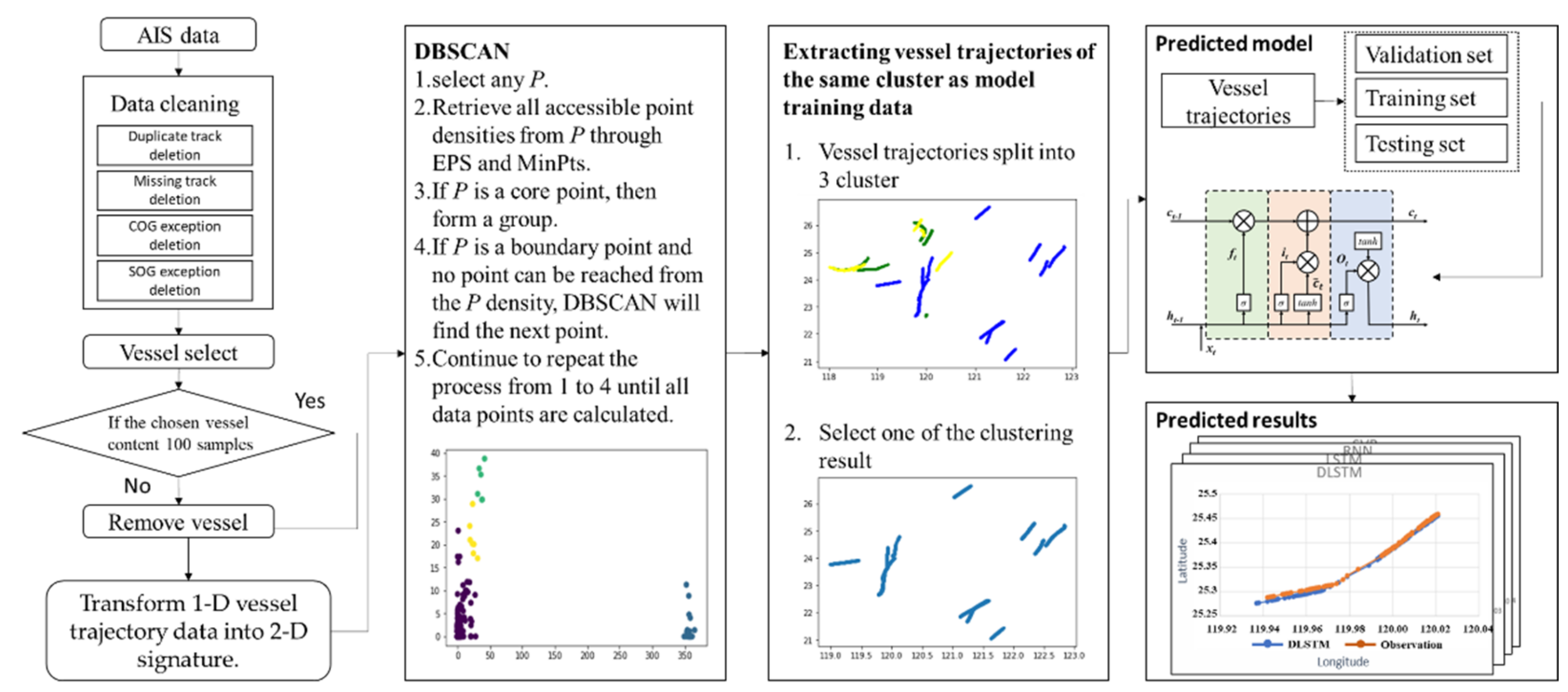
3. Method
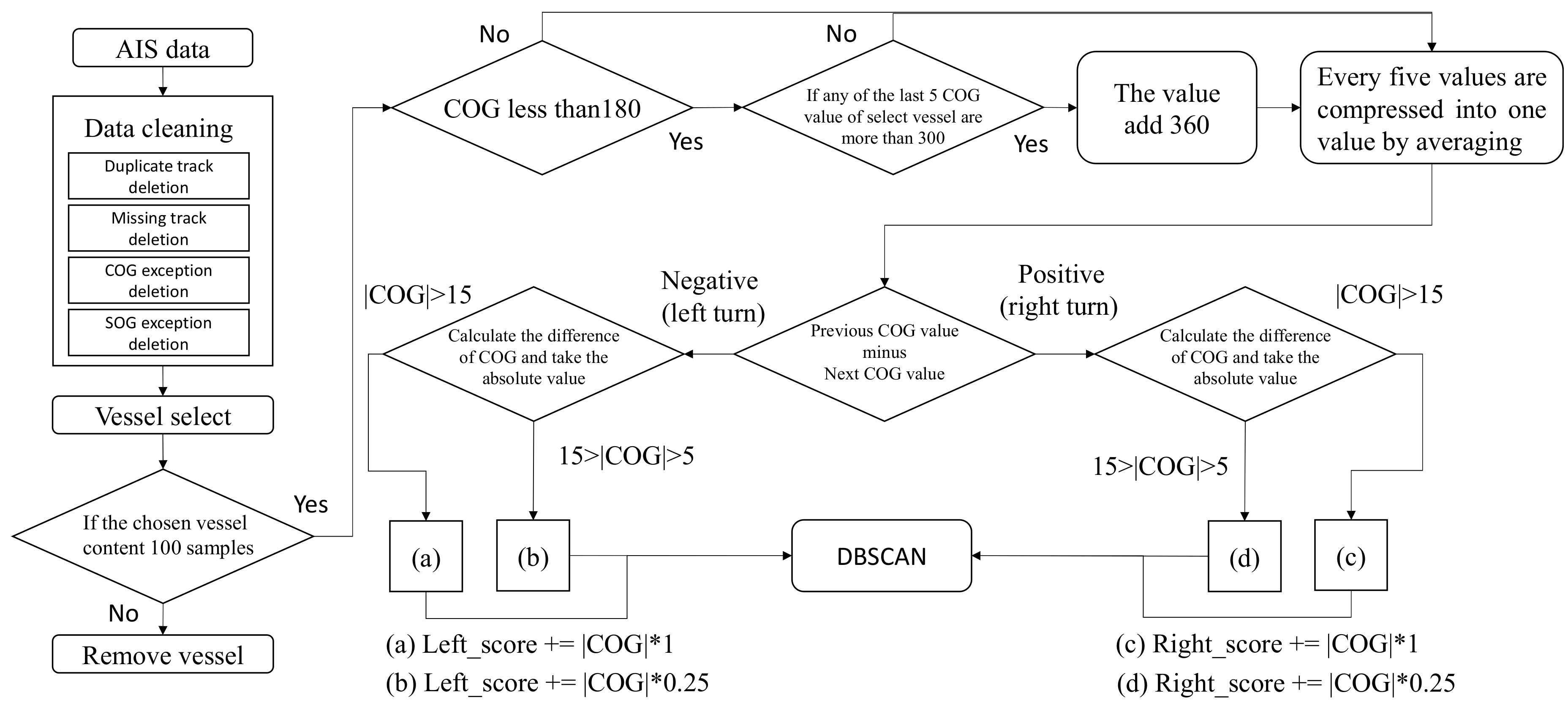
3.1. Study Design
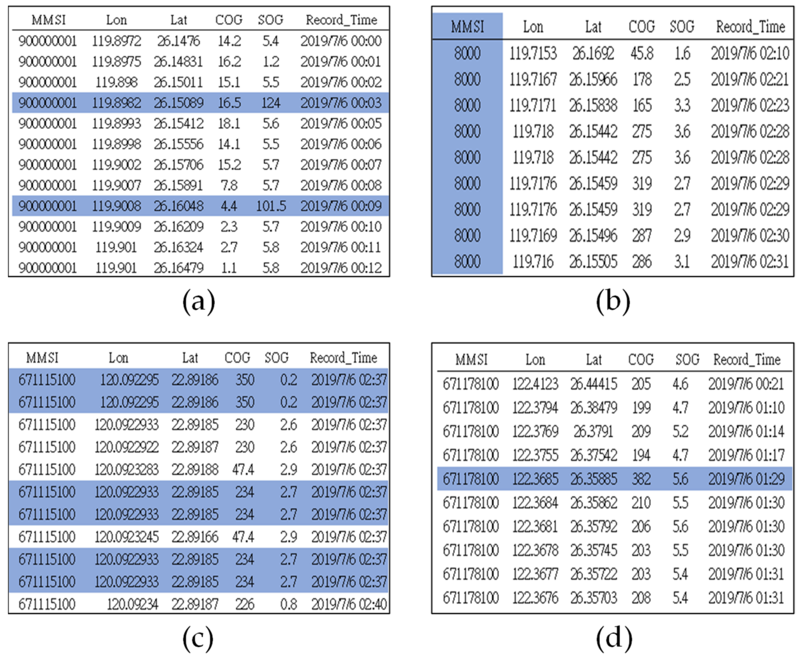
3.1.1. Collection of Data on Vessel Trajectory, Speed, Course, and Other Features
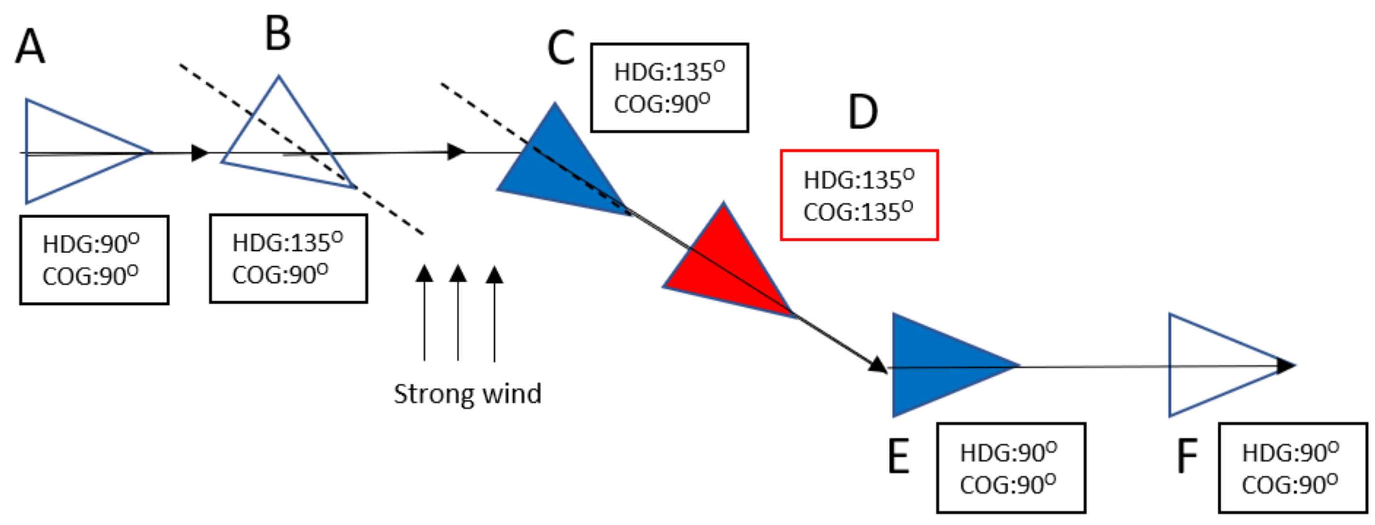
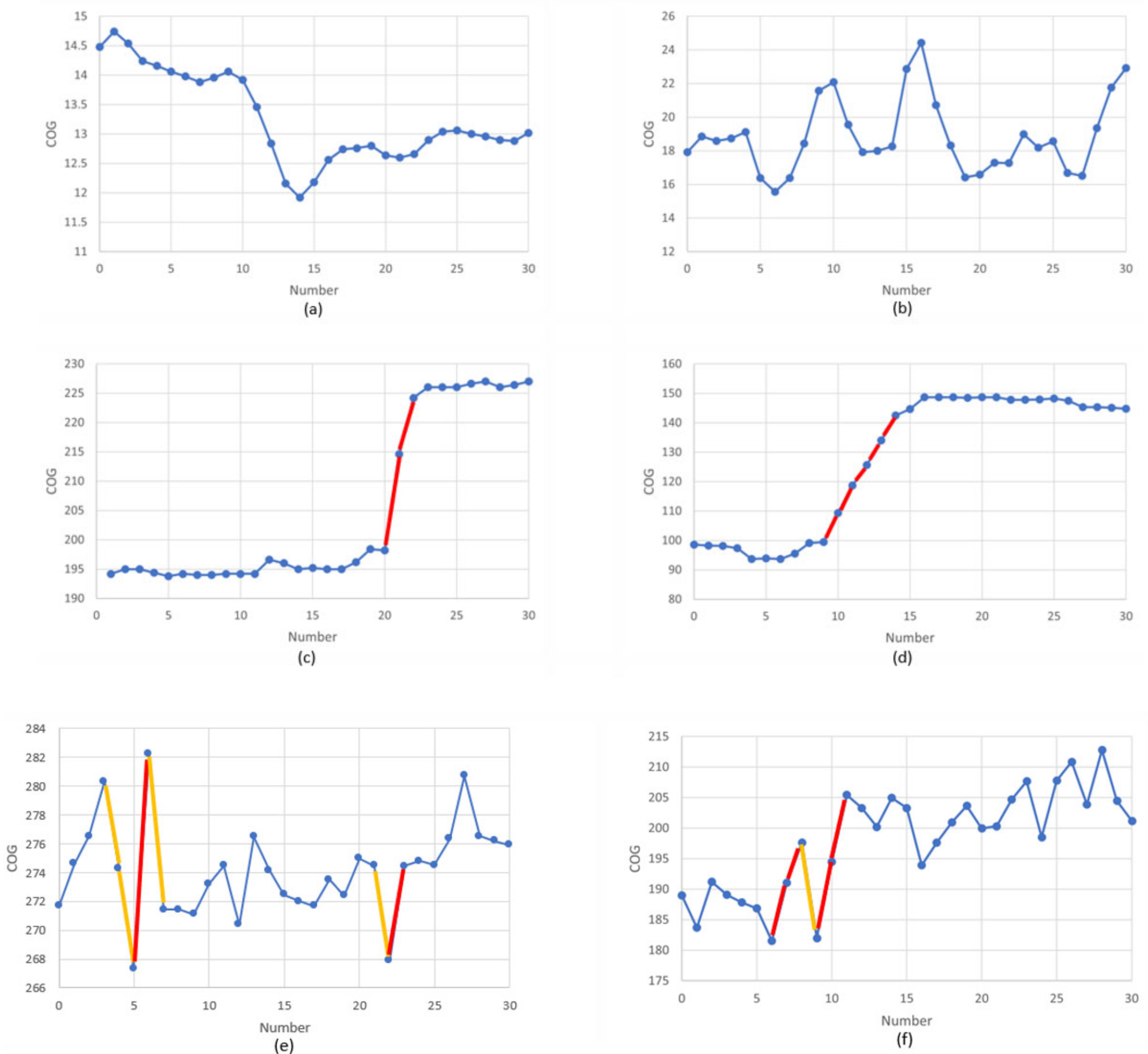
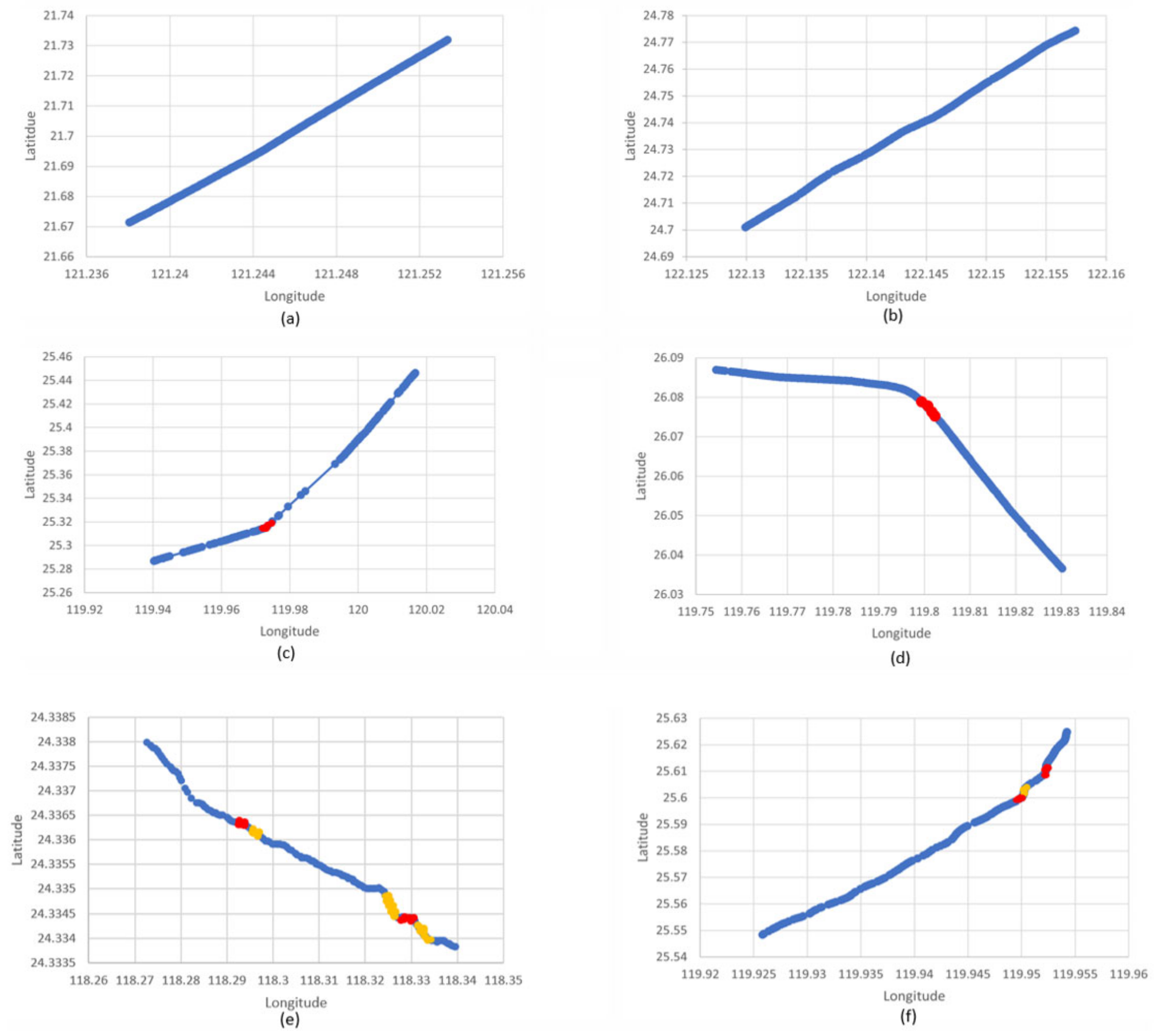
3.1.2. Data Cleaning through Track Separation and Outlier Deletion
3.2. Trajectory Similarity Measurement
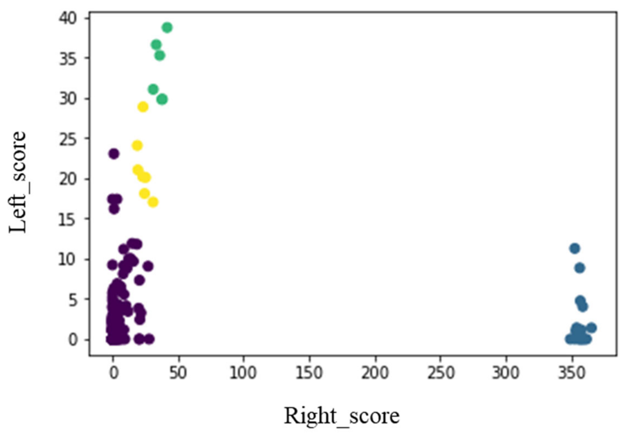
3.3. DBSCAN
| Algorithm 1 DBSCAN |
| DBSCAN (eps, minpts, D) |
| mark all patterns in D as unvisited |
| cluid ← 1 |
| for each unvisited pattern x in D |
| do |
| Z ← Find Neighbours (x, eps, minpts) |
| if |Z| < minpts |
| mark x as noise |
| else |
| mark x and each pattern of Z with cluid |
| queue_list ← all unvisited patterns of Z |
| until queue_list is empty |
| do |
| y ← delete a pattern from queue_list |
| Z ← Find Neighbours (x, eps, minpts) |
| if |Z| ≧ minpts |
| for each pattern w in Z |
| mark w with cluid |
| if w is unvisited |
| queue_list ← w U queue_list |
| end for |
| end if |
| mark x as visited |
| cluid ← cluid + 1 |
| end for |
| Output all patterns in D marked with cluid or noise |
3.4. Support Vector Regression (SVR)
3.5. Recurrent Neural Network (RNN)
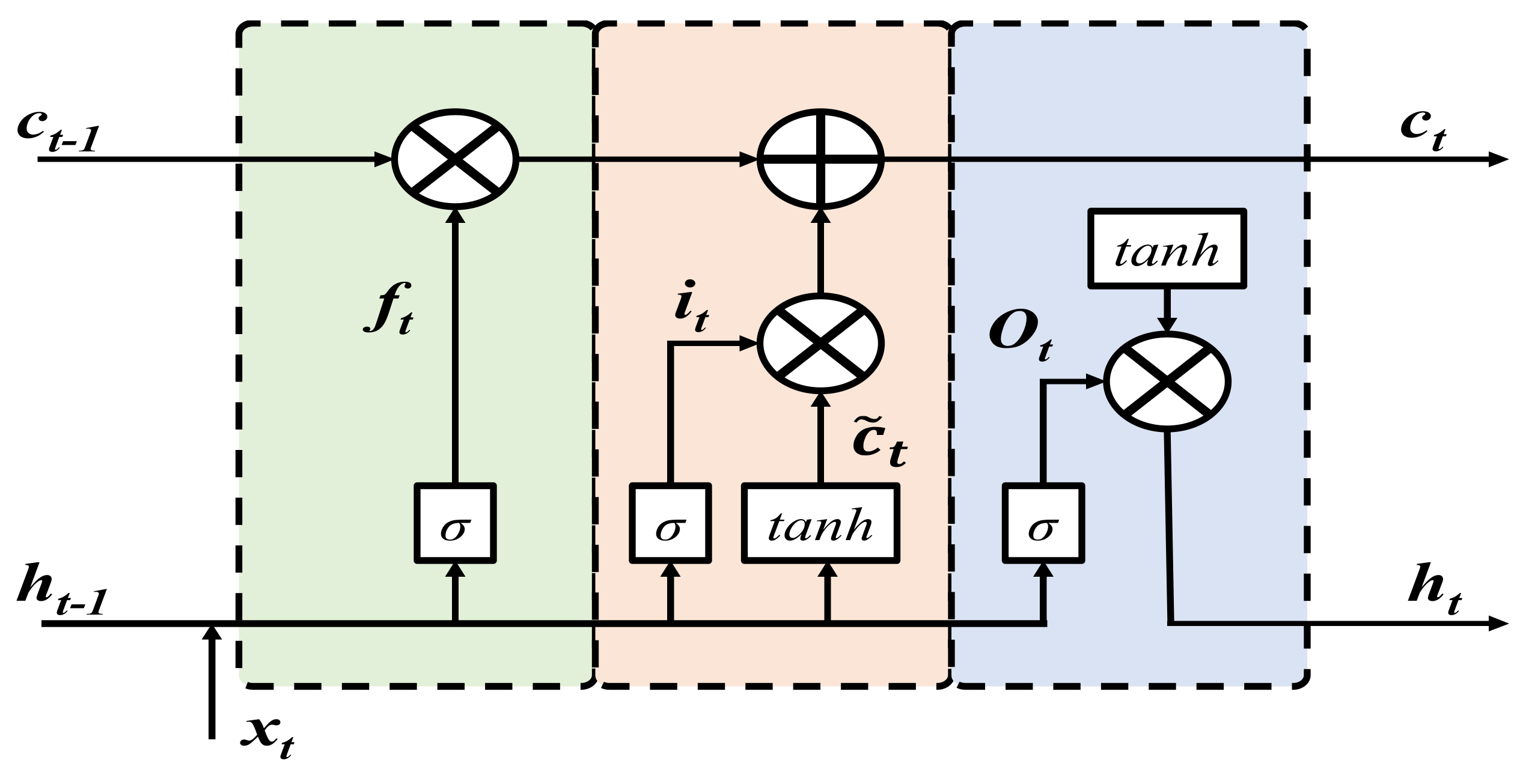
3.6. Long Short-Term Memory (LSTM)
3.7. Performance Verification
4. Result and Discussions
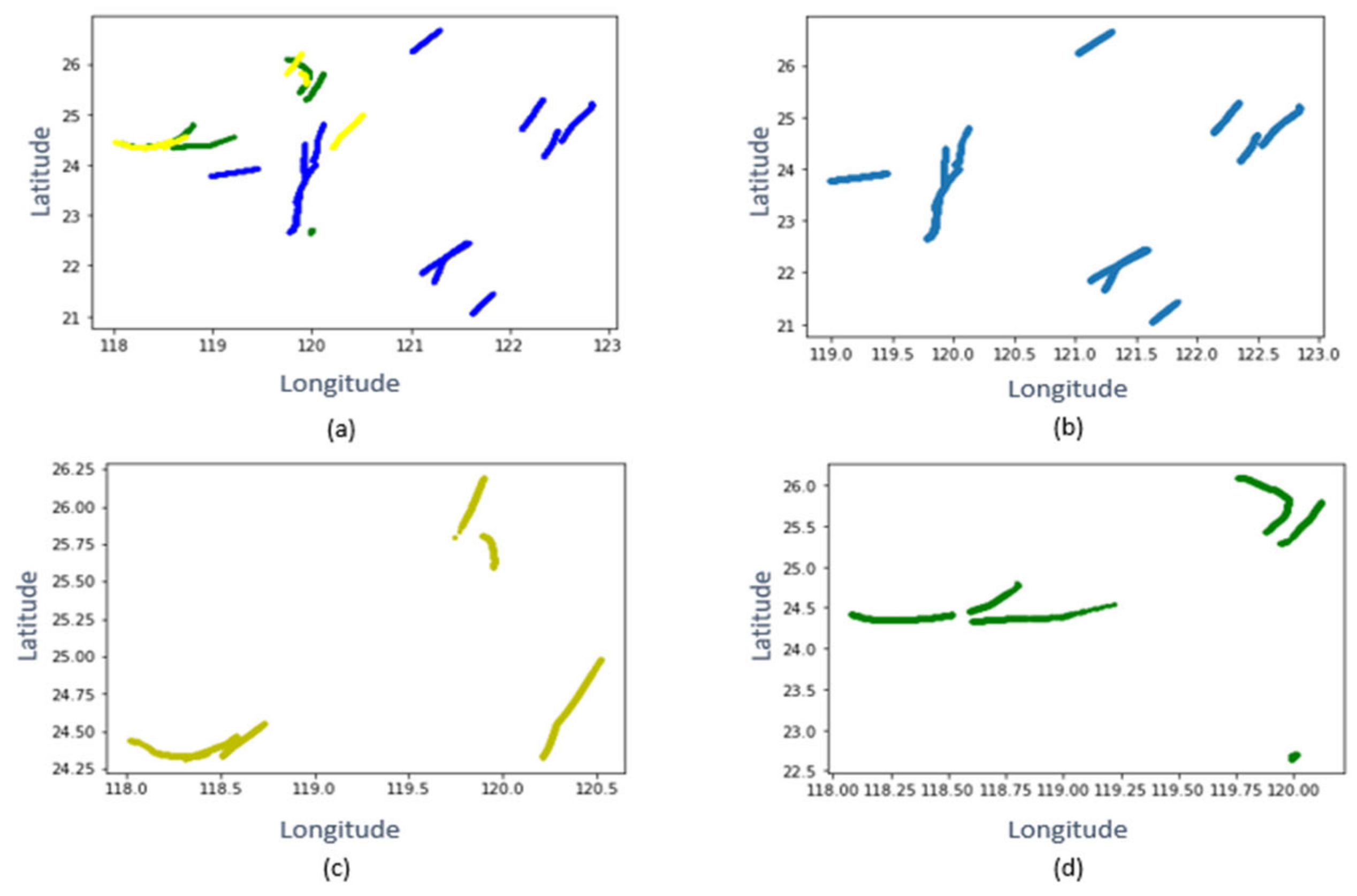
4.1. Clustering
4.2. Parameter Settings
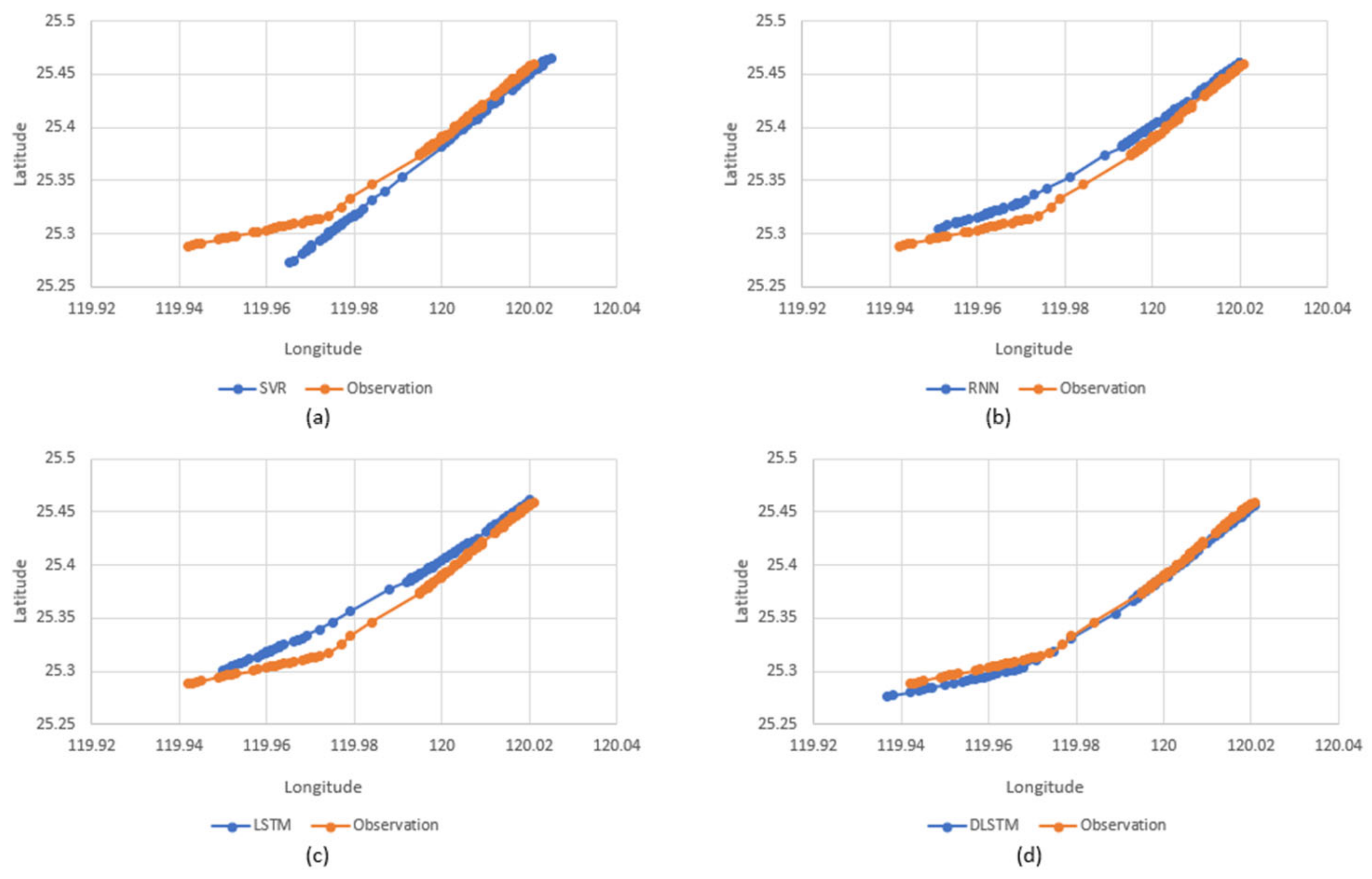
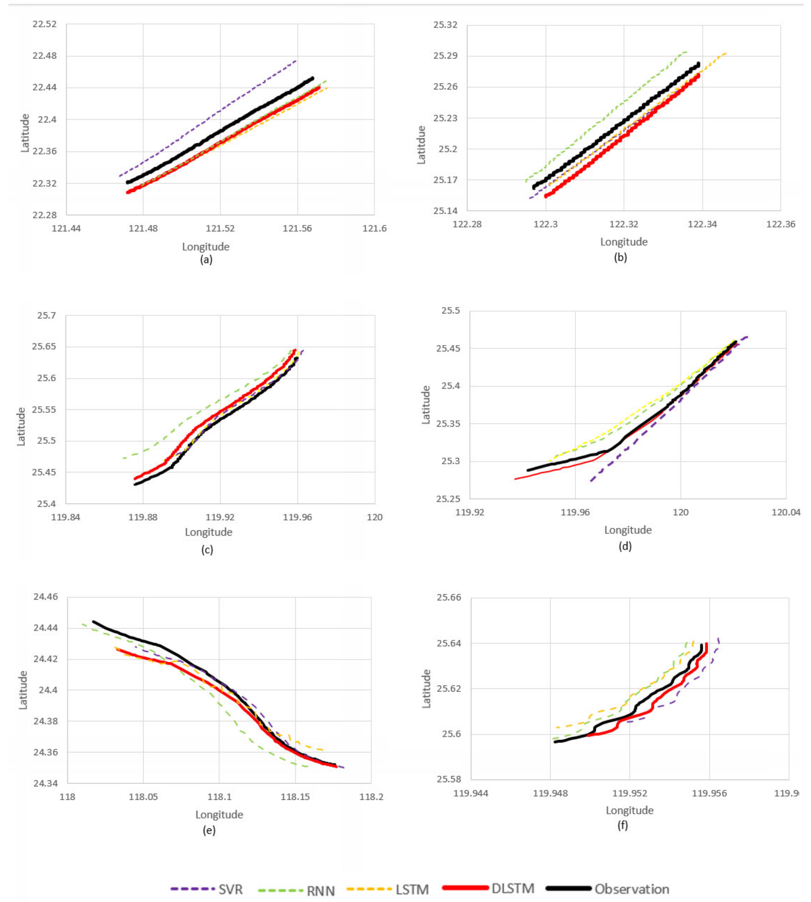
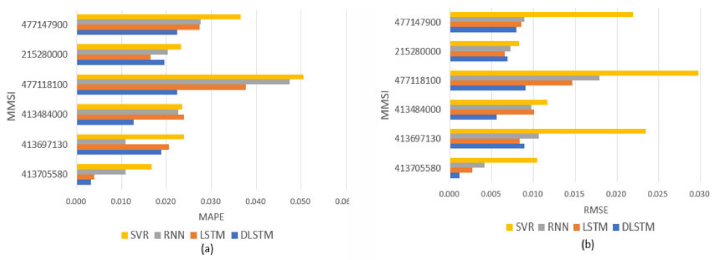
4.3. Trajectory Prediction Results
5. Conclusions
Author Contributions
Funding
Institutional Review Board Statement
Informed Consent Statement
Data Availability Statement
Conflicts of Interest
References
- Tu, E.; Zhang, G.; Rachmawati, L.; Rajabally, E.; Huang, G.-B. Exploiting AIS data for intelligent maritime navigation: A comprehensive survey from data to methodology. IEEE Trans. Intell. Transp. Syst. 2017, 19, 1559–1582. [Google Scholar] [CrossRef]
- Sirimanne, S.N.; Hoffman, J.; Juan, W.; Asariotis, R.; Assaf, M.; Ayala, G.; Benamara, H.; Chantrel, D.; Hoffmann, J.; Premti, A. Review of maritime transport 2019. In Proceedings of the United Nations Conference on Trade and Development, Geneva, Switzerland, 30 October 2019. [Google Scholar]
- Harati-Mokhtari, A.; Wall, A.; Brooks, P.; Wang, J. Automatic Identification System (AIS): Data reliability and human error implications. J. Navig. 2007, 60, 373–389. [Google Scholar] [CrossRef]
- Norris, A. AIS implementation–Success or failure? J. Navig. 2007, 60, 1–10. [Google Scholar] [CrossRef]
- Sanchez-Gonzalez, P.-L.; Díaz-Gutiérrez, D.; Leo, T.J.; Núñez-Rivas, L.R. Toward digitalization of maritime transport? Sensors 2019, 19, 926. [Google Scholar] [CrossRef] [PubMed]
- Jurdana, I.; Krylov, A.; Yamnenko, J. Use of artificial intelligence as a problem solution for maritime transport. J. Mar. Sci. Eng. 2020, 8, 201. [Google Scholar] [CrossRef]
- Alahi, A.; Goel, K.; Ramanathan, V.; Robicquet, A.; Fei-Fei, L.; Savarese, S. Social lstm: Human trajectory prediction in crowded spaces. In Proceedings of the IEEE Conference on Computer Vision and Pattern Recognition, Las Vegas, NV, USA, 27 June 2016; pp. 961–971. [Google Scholar]
- Park, S.H.; Kim, B.; Kang, C.M.; Chung, C.C.; Choi, J.W. Sequence-to-sequence prediction of vehicle trajectory via LSTM encoder-decoder architecture. In Proceedings of the 2018 IEEE Intelligent Vehicles Symposium (IV), Changshu, China, 26–30 June 2018; pp. 1672–1678. [Google Scholar]
- Xiaopeng, T.; Xu, C.; Lingzhi, S.; Zhe, M.; Qing, W. Vessel trajectory prediction in curving channel of inland river. In Proceedings of the 2015 International Conference on Transportation Information and Safety, Wuhan, China, 25–28 June 2015; pp. 706–714. [Google Scholar]
- Wang, L.; Zhang, L.; Yi, Z. Trajectory predictor by using recurrent neural networks in visual tracking. IEEE Trans. Cybern. 2017, 47, 3172–3183. [Google Scholar] [CrossRef]
- Lee, H.-T.; Lee, J.-S.; Yang, H.; Cho, I.-S. An AIS Data-Driven Approach to Analyze the Pattern of Ship Trajectories in Ports Using the DBSCAN Algorithm. Appl. Sci. 2021, 11, 799. [Google Scholar] [CrossRef]
- Zhang, D.; Ren, Q.; Su, D. A Novel Authentication Methodology to Detect Counterfeit PCB Using PCB Trace-Based Ring Oscillator. IEEE Access 2021, 9, 28525–28539. [Google Scholar] [CrossRef]
- Hochreiter, S.; Schmidhuber, J. Long short-term memory. Neural Comput. 1997, 9, 1735–1780. [Google Scholar] [CrossRef] [PubMed]
- Ryu, J.; Kamata, S.-I. An efficient computational algorithm for Hausdorff distance based on points-ruling-out and systematic random sampling. Pattern Recognit. 2021, 114, 107857. [Google Scholar] [CrossRef]
- Du, J.; Wu, F.; Yin, J.; Liu, C.; Gong, X. Polyline simplification based on the artificial neural network with constraints of generalization knowledge. Cartogr. Geogr. Inf. Sci. 2022, 49, 313–337. [Google Scholar] [CrossRef]
- Deng, D. DBSCAN clustering algorithm based on density. In Proceedings of the 2020 7th International Forum on Electrical Engineering and Automation (IFEEA), Hefei, China, 25–27 September 2020; pp. 949–953. [Google Scholar]
- Drucker, H.; Burges, C.J.; Kaufman, L.; Smola, A.; Vapnik, V. Support vector regression machines. Adv. Neural Inf. Processing Syst. 1996, 9, 155–161. [Google Scholar]
- Nguyen, D.-D.; Le Van, C.; Ali, M.I. Vessel trajectory prediction using sequence-to-sequence models over spatial grid. In Proceedings of the 12th ACM International Conference on Distributed and Event-Based Systems, Hamilton, New Zealand, 25 June 2018; pp. 258–261. [Google Scholar]
- Borkowski, P. The Ship Movement Trajectory Prediction Algorithm Using Navigational Data Fusion. Sensors 2017, 17, 1432. [Google Scholar] [CrossRef] [PubMed]
- Meng, S.; Wang, H.; Lu, W.; Wang, Z.; Li, Y. Drift trajectory model of the unpowered vessel on the sea and its application in the drift simulation of the Sanchi oil tanker. Oceanol. Limnol. Sin. 2018, 49, 242–250. [Google Scholar]
- Murray, B.; Perera, L.P. A data-driven approach to vessel trajectory prediction for safe autonomous ship operations. In Proceedings of the 2018 13th International Conference on Digital Information Management, Berlin, Germany, 24–26 September 2018; pp. 240–247. [Google Scholar]
- Yan, Z. Traj-ARIMA: A spatial-time series model for network-constrained trajectory. In Proceedings of the Third International Workshop on Computational Transportation Science, San Jose, CA, USA, 2 November 2010; pp. 11–16. [Google Scholar]
- Qi, L.; Zheng, Z. Trajectory prediction of vessels based on data mining and machine learning. J. Digit. Inf. Manag. 2016, 14, 33–40. [Google Scholar]
- Zhang, L.; Meng, Q. Probabilistic ship domain with applications to ship collision risk assessment. Ocean Eng. 2019, 186, 106130. [Google Scholar] [CrossRef]
- Wang, C.; Ren, H.; Li, H. Vessel trajectory prediction based on AIS data and bidirectional GRU. In Proceedings of the 2020 International Conference on Computer Vision, Image and Deep Learning, Chongqing, China, 10–12 July 2020; pp. 260–264. [Google Scholar]
- Huang, C.; Wang, J.; Chen, X.; Cao, J. Bifurcations in a fractional-order BAM neural network with four different delays. Neural Netw. 2021, 141, 344–354. [Google Scholar] [CrossRef] [PubMed]
- Yang, W.; Yu, W.; Cao, J.; Alsaadi, F.E.; Hayat, T. Almost automorphic solution for neutral type high-order Hopfield BAM neural networks with time-varying leakage delays on time scales. Neurocomputing 2017, 267, 241–260. [Google Scholar] [CrossRef]
- Xu, C.; Zhang, W.; Aouiti, C.; Liu, Z.; Yao, L. Further analysis on dynamical properties of fractional-order bi-directional associative memory neural networks involving double delays. Math. Methods Appl. Sci. 2022. [Google Scholar] [CrossRef]
- Xu, Z.; Zeng, W.; Chen, L.; Chu, X. Aircraft Trajectory Prediction Using Social LSTM Neural Network. In Proceedings of the CICTP 2021, Xi’an, China, 16–19 December 2021; pp. 87–97. [Google Scholar]
- Semerdjiev, E.; Mihaylova, L. Variable-and fixed-structure augmented interacting multiple model algorithms for manoeuvring ship tracking based on new ship models. Int. J. Appl. Math. Comput. Sci. 2000, 10, 591–604. [Google Scholar]
- Tusell, F. Kalman filtering in R. J. Stat. Softw. 2011, 39, 1–27. [Google Scholar] [CrossRef]
- De Vries, G.K.D.; Van Someren, M. Machine learning for vessel trajectories using compression, alignments and domain knowledge. Expert Syst. Appl. 2012, 39, 13426–13439. [Google Scholar] [CrossRef]
- Kim, J.-S. Vessel target prediction method and dead reckoning position based on SVR seaway model. Int. J. Fuzzy Logic Intell. Syst. 2017, 17, 279–288. [Google Scholar] [CrossRef]
- Rumelhart, D.E.; Hinton, G.E.; Williams, R.J. Learning representations by back-propagating errors. Nature 1986, 323, 533–536. [Google Scholar] [CrossRef]
- Ribeiro, A.H.; Tiels, K.; Aguirre, L.A.; Schön, T. Beyond exploding and vanishing gradients: Analysing RNN training using attractors and smoothness. In Proceedings of the International Conference on Artificial Intelligence and Statistics, Online, 26–28 August 2020; pp. 2370–2380. [Google Scholar]
- Zhou, C.; Sun, C.; Liu, Z.; Lau, F. A C-LSTM neural network for text classification. arXiv 2015, arXiv:1511.08630. [Google Scholar]
- Chen, K.; Zhou, Y.; Dai, F. A LSTM-based method for stock returns prediction: A case study of China stock market. In Proceedings of the 2015 IEEE International Conference on Big Data (Big Data), Santa Clara, CA, USA, 29 October–1 November 2015; pp. 2823–2824. [Google Scholar]
- Yang, C.-H.; Wu, C.-H.; Shao, J.-C.; Wang, Y.-C.; Hsieh, C.-M. AIS-Based Intelligent Vessel Trajectory Prediction Using Bi-LSTM. IEEE Access 2022, 10, 24302–24315. [Google Scholar] [CrossRef]
- Kumar, K.M.; Reddy, A.R.M. A fast DBSCAN clustering algorithm by accelerating neighbor searching using Groups method. Pattern Recognit. 2016, 58, 39–48. [Google Scholar] [CrossRef]
- Tran, T.N.; Drab, K.; Daszykowski, M. Revised DBSCAN algorithm to cluster data with dense adjacent clusters. Chemom. Intell. Lab. Syst. 2013, 120, 92–96. [Google Scholar] [CrossRef]
- Vapnik, V.; Golowich, S.E.; Smola, A.J. Support vector method for function approximation, regression estimation and signal processing. In Proceedings of the Advances in Neural Information Processing Systems, Denver, DC, USA, 2–5 December 1997; pp. 281–287. [Google Scholar]
- Ceperic, E.; Ceperic, V.; Baric, A. A strategy for short-term load forecasting by support vector regression machines. IEEE Trans. Power Syst. 2013, 28, 4356–4364. [Google Scholar] [CrossRef]
- Mehr, A.D.; Nourani, V.; Khosrowshahi, V.K.; Ghorbani, M.A. A hybrid support vector regression—Firefly model for monthly rainfall forecasting. Int. J. Environ. Sci. Technol. 2019, 16, 335–346. [Google Scholar] [CrossRef]
- Bengio, Y.; Simard, P.; Frasconi, P. Learning long-term dependencies with gradient descent is difficult. IEEE Trans. Neural Netw. 1994, 5, 157–166. [Google Scholar] [CrossRef]
- Pascanu, R.; Mikolov, T.; Bengio, Y. On the difficulty of training recurrent neural networks. In Proceedings of the International Conference on Machine Learning, Atlanta GA USA, 16 June 2013; pp. 1310–1318. [Google Scholar]
- Cho, K.; Van Merriënboer, B.; Bahdanau, D.; Bengio, Y. On the properties of neural machine translation: Encoder-decoder approaches. arXiv 2014, arXiv:1409.1259. [Google Scholar]
- Kratzert, F.; Klotz, D.; Brenner, C.; Schulz, K.; Herrnegger, M. Rainfall–runoff modelling using long short-term memory (LSTM) networks. Hydrol. Earth Syst. Sci. 2018, 22, 6005–6022. [Google Scholar] [CrossRef]


| Index | MMSI | Left_Score | Right_Score |
|---|---|---|---|
| 1 | 538006353 | 0 | 0 |
| 2 | 538006573 | 0 | 1.52 |
| 3 | 538005414 | 4.448 | 4.252 |
| 4 | 538004214 | 1.44 | 0 |
| 5 | 477946000 | 39.36 | 3.84 |
| 6 | 477943000 | 1.116 | 6.16 |
| 7 | 477938400 | 8.948 | 9.14 |
| 8 | 477800200 | 20.32 | 0 |
| 9 | 477698600 | 1.964 | 1.916 |
| MMSI | Cluster | Cluster Data | AIS Data | DLSTM Train Data | Train Data | Test Data |
|---|---|---|---|---|---|---|
| 477147900 | 1 | 15,372 | 1819 | 13,553 | 1455 | 364 |
| 215280000 | 1188 | 14,184 | 950 | 238 | ||
| 477118100 | 2 | 5662 | 1500 | 4162 | 1200 | 300 |
| 413484000 | 786 | 4876 | 629 | 157 | ||
| 413697130 | 3 | 4004 | 736 | 3268 | 589 | 147 |
| 413705580 | 533 | 3471 | 426 | 107 |
| MMSI | Layer1 | Layer2 | Lr | Epoch | Batch | MAPE | RMSE |
|---|---|---|---|---|---|---|---|
| 413697130 | 50 | 0.00001 | 250 | 128 | 0.03 | 0.04 | |
| 80 | 0.026 | 0.01 | |||||
| 128 | 0.04 | 0.019 | |||||
| 256 | 0.03 | 0.01 | |||||
| 80 | 50 | 0.019 | 0.009 | ||||
| 80 | 0.14 | 0.04 | |||||
| 128 | 0.18 | 0.06 | |||||
| 256 | 0.03 | 0.03 |
| Input | LSTM_1 | LSTM_2 | Output | Activation Function | Learning Rate | Epochs |
|---|---|---|---|---|---|---|
| 238 | 128 | 50 | 1 | Adam | 1 × 10⁻⁵ | 300 |
| MMSI | Clustering | Criteria | SVR | RNN | LSTM |
|---|---|---|---|---|---|
| 477147900 | 1 | MAPE | 0.14 | 0.3 | 0.2 |
| RMSE | 0.06 | 0.09 | 0.09 | ||
| R2 | 0.25 | 0.07 | 0.01 | ||
| 215280000 | 1 | MAPE | 0.2 | 0.16 | 0.34 |
| RMSE | 0.09 | 0.1 | 0.15 | ||
| R2 | −0.5 | −1.36 | −3.5 | ||
| 477118100 | 2 | MAPE | 0.15 | 0.16 | 0.41 |
| RMSE | 0.06 | 0.15 | 0.2 | ||
| R2 | 0.27 | −5 | −9.7 | ||
| 413484000 | 2 | MAPE | 0.18 | 0.37 | 0.11 |
| RMSE | 0.065 | 0.15 | 0.04 | ||
| R2 | 0.5 | −5 | 0.19 | ||
| 413697130 | 3 | MAPE | 0.11 | 0.37 | 0.49 |
| RMSE | 0.07 | 0.14 | 0.217 | ||
| R2 | −0.6 | −24 | −46 | ||
| 413705580 | 3 | MAPE | 0.12 | 0.12 | 0.13 |
| RMSE | 0.05 | 0.1 | 0.05 | ||
| R2 | −3.6 | −3.9 | −17.3 |
| MMSI | Clustering | Criteria | SVR | RNN | LSTM | DLSTM |
|---|---|---|---|---|---|---|
| 477147900 | 1 | MAPE | 0.036 | 0.028 | 0.027 | 0.022 |
| RMSE | 0.022 | 0.009 | 0.009 | 0.008 | ||
| R2 | 0.881 | 0.941 | 0.950 | 0.963 | ||
| 215280000 | 1 | MAPE | 0.023 | 0.020 | 0.016 | 0.016 |
| RMSE | 0.008 | 0.007 | 0.007 | 0.007 | ||
| R2 | 0.889 | 0.935 | 0.942 | 0.950 | ||
| 477118100 | 2 | MAPE | 0.051 | 0.047 | 0.038 | 0.022 |
| RMSE | 0.030 | 0.018 | 0.015 | 0.009 | ||
| R2 | 0.857 | 0.870 | 0.910 | 0.986 | ||
| 413484000 | 2 | MAPE | 0.023 | 0.023 | 0.024 | 0.013 |
| RMSE | 0.012 | 0.010 | 0.010 | 0.006 | ||
| R2 | 0.880 | 0.964 | 0.964 | 0.986 | ||
| 413697130 | 3 | MAPE | 0.024 | 0.011 | 0.021 | 0.019 |
| RMSE | 0.023 | 0.011 | 0.008 | 0.009 | ||
| R2 | 0.901 | 0.944 | 0.948 | 0.954 | ||
| 413705580 | 3 | MAPE | 0.017 | 0.011 | 0.004 | 0.003 |
| RMSE | 0.010 | 0.004 | 0.003 | 0.001 | ||
| R2 | 0.752 | 0.889 | 0.938 | 0.952 | ||
| Average | - | MAPE | 0.029 | 0.023 | 0.022 | 0.016 |
| RMSE | 0.018 | 0.010 | 0.008 | 0.007 | ||
| R2 | 0.860 | 0.924 | 0.942 | 0.965 | ||
| p-value | - | MAPE | 0.006 | 0.189 | 0.131 | - |
| RMSE | 0.006 | 0.028 | 0.066 | - |
Publisher’s Note: MDPI stays neutral with regard to jurisdictional claims in published maps and institutional affiliations. |
© 2022 by the authors. Licensee MDPI, Basel, Switzerland. This article is an open access article distributed under the terms and conditions of the Creative Commons Attribution (CC BY) license (https://creativecommons.org/licenses/by/4.0/).
Share and Cite
Yang, C.-H.; Lin, G.-C.; Wu, C.-H.; Liu, Y.-H.; Wang, Y.-C.; Chen, K.-C. Deep Learning for Vessel Trajectory Prediction Using Clustered AIS Data. Mathematics 2022, 10, 2936. https://doi.org/10.3390/math10162936
Yang C-H, Lin G-C, Wu C-H, Liu Y-H, Wang Y-C, Chen K-C. Deep Learning for Vessel Trajectory Prediction Using Clustered AIS Data. Mathematics. 2022; 10(16):2936. https://doi.org/10.3390/math10162936
Chicago/Turabian StyleYang, Cheng-Hong, Guan-Cheng Lin, Chih-Hsien Wu, Yen-Hsien Liu, Yi-Chuan Wang, and Kuo-Chang Chen. 2022. "Deep Learning for Vessel Trajectory Prediction Using Clustered AIS Data" Mathematics 10, no. 16: 2936. https://doi.org/10.3390/math10162936