1. Introduction
Let be an n-vertex simple and a connected graph with size e. We represent the edge set and the vertex set of by and , respectively. The degree of is the number of adjacent vertices to h in , and it is represented by . For , is the set of all neighbors of h in . For the two given vertices, , we describe their distance by the length of the shortest path among and in , and . For a vertex , its eccentricity is written as . A vertex h is named as a well-connected node in an n-vertex graph if and obviously its eccentricity will be 1. We represent the set of all well-connected vertices of with , and represents its cardinality. The unique vertex of is considered to be a well-connected vertex, and is a well-connected graph. Let be a complete l-partite graph with an number of vertices. The set of vertices can be divided up into subsets such that there is no edge between the vertices of the same set , . We use the notions and for the n-vertex complete graph and cycle, respectively.
In mathematical chemistry and chemical graph theory, a molecular (or chemical) graph is a representation of the structural formula of a chemical compound in the form of graph theory. Its vertices are presented by the types of the corresponding atoms, and its edges are presented by the kinds of its bonds. A molecular graph has been used in the prediction of properties relevant to the drug discovery and optimization process. For example, knowledge discovery can be used for the identification of lead compounds in pharmaceutical data matching. A molecular descriptor is a numerical parameter of a graph that distinguishes its topology. Topological invariants have constructed numerous applications in pharmaceutical drug design, QSAR/QSPR study, chemical documentations and isomer discrimination. The eccentric-connectivity index of
is a new distance-related descriptor that was designed by Sharma et al. [
1] and is described as:
In the present-day literature, a modification of
has been found and mentioned as the total-eccentricity
index.It is described as:
The eccentric connectivity polynomial
is the continuation of
, which was initiated by Ashraf and Jalali [
2], and described as:
The total eccentricity polynomial of
is interpreted as follows:
It is straightforward that the total-eccentricity and eccentric-connectivity indices of can be acquired from the parallel polynomials by taking their first derivative at .
In theoretical chemistry, the research of an eccentric-connectivity polynomial for chemical structures has become an attractive area in recent years. The eccentric distance sum of
was proposed by Gupta et al. [
3] and was construed as follows:
This index suggests a massive capability for structure-activity and structure-property connections and has exhibited a great predictive power in pharmaceutical properties. It also shows vast discriminating power with reference to physical and biological characterizations [
3]. From [
3], the eccentric-distance sum gives a better result in the study of some structure-activities and quantitative structure-properties, more than the corresponding results acquired by using the Wiener index. WIth the help of the eccentric-distance sum index and anti-HIV activity of dihydroseselins, the researchers investigated and facilitated the development of potent and safe anti-HIV agents. The accuracy of prediction was found to be more than 88 percent with regard to anti-HIV activity. The eccentric distance sum exhibited a much better correlation and fewer average errors than Wiener’s topological index. Recently, the mathematical aspects of the
have been examined. The eccentric-distance sum polynomial of
is proposed as:
Graph operations play a valuable part in many combinatorial characterizations, graph decompositions into isomorphic subgraphs in pure mathematics, and also applied mathematics. The study of finding the topological invariants of different molecular graph structures by the use of the topological invariants of graph operations has valuable importance these days. There are many complicated molecular structures, such as
-nanotorus, Hamming graphs, closed fence graphs, etc., for which it is so difficult to find their topological indices and polynomials, so for this purpose, the researchers can use graph operations. Azari and Iranmanesh [
4] determined this index for some prominent graph operations. Došlić and Hosseinzadeh [
5] computed its corresponding polynomial for various graph operations. Yu et al. [
6] worked out this index for unicyclic graphs and trees. Hua et al. [
7] secured the bound on the eccentric-distance sum of cacti. Hua et al. [
8] considered the graphs having the smallest eccentric-distance sum with graph parameters. Ilić et al. [
9] computed several bounds of
in the form of the different graph invariants. Geng et al. [
10] worked out the
of the trees with some given parameters. For more information on different aspects of indices and polynomials, one can see [
11,
12,
13,
14,
15,
16,
17,
18,
19,
20].
In this article, we are interested in acquiring the eccentric-distance sum polynomial of graph products. Then, we perform our findings to determine the eccentric-distance sum polynomial of certain significant categories of graphs in the form of factors of graph products.
Proposition 1. Let and be the n-vertex complete graph and cycle, respectively. Then
- 1
.
- 2
.
- 3
- 4
2. Join
The join of and graphs is recognized as , which consists of edge sets and disjoint vertex sets , where . It is graph union including all the links joining and . For , we represent by . First, we give a lemma, which plays a vital role in the solution of the leading result.
Lemma 1. Let be graphs with and , . Then, for the vertices , we have the following:
- 1
- 2
Next, we calculate the eccentric distance sum polynomial of with the help of Lemma 1.
Theorem 1. For a graph , where , , and , we have Proof. Note that if
, then
, for
. The degree of
is
, where
and
. Now, by Equation (
1) and Lemma 1, we have:
After some simple computations, we can get above the expression. This finishes the proof. □
Similarly, the following corollaries can be easily derived from Theorem 1, so we omitted their proofs.
Corollary 1. For graphs and with and , where or q, we have Corollary 2. Let , and let denote the k copies of with order n and size e. Then, Example 1. It is easy to observe that, for the given complete m-partite graph , using Theorem 1, we acquire For , we have complete bipartite graph on vertices. Therefore, .
Example 2. The cone graph is described as , and its eccentric-distance sum polynomial is .
For a given graph , the suspension of is defined as . The following result follows from Corollary 1.
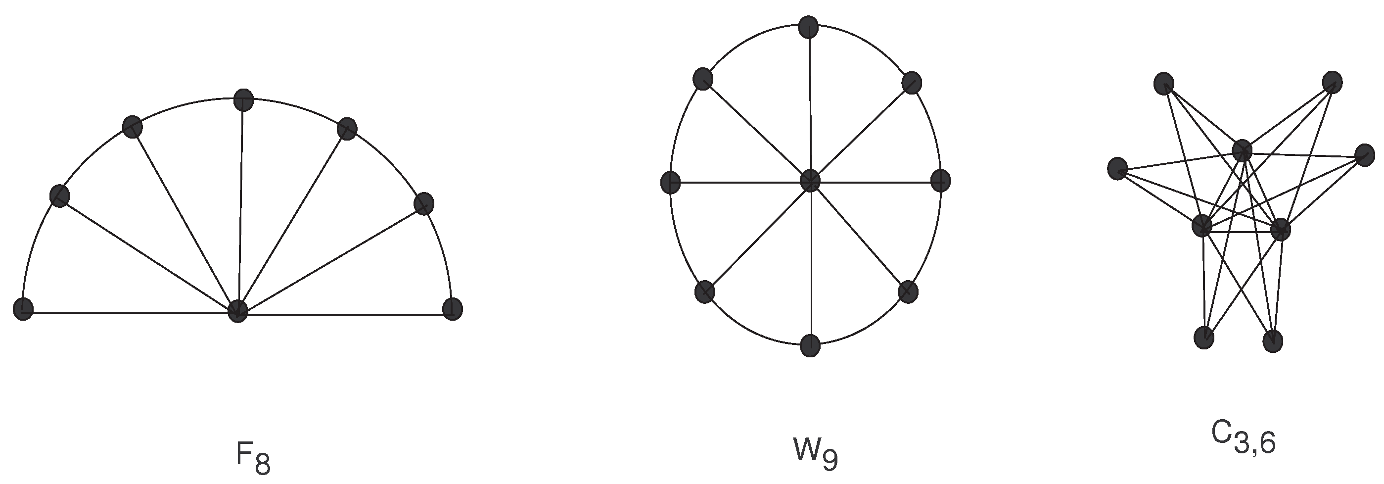
Example 3. For a graph with and , we have Star graph , fan graph and wheel graph on vertices are the suspensions of the empty graph, , and , respectively (see Figure 1). Therefore, by (2), we obtain the following: 3. Cartesian Product
Here, we denote the Cartesian product of and by It has vertex set and if and , or and . In the beginning, we give an essential lemma that relates the properties of the Cartesian product.
Lemma 2. For and with and , where or q, we have the following:
- (a)
- (b)
Now, we give the expression for the eccentric-distance sum polynomial of , in the form of eccentric-distance sum, and total eccentricity polynomials of , for .
Theorem 2. Let be graphs with , , , and . Then we have Proof. By using Lemma 2 and Equation (
1), we obtain
Again, by Lemma 2, we have:
This finishes the proof. □
Example 4. Let , for some integers , denote a -nanotorus. Then, by using Theorem 2 and Proposition 1, we obtain Example 5. The Hamming graph is a connected graph with k-tuples vertices , where , , , and is an edge, if the interrelated tuples differ in exactly one place and are commonly expressed as . By using Theorem 2 and Proposition 1, we obtain: If , then the Hamming graph is famous as a k-dimensional hypercube graph, and it is symbolized by (see Figure 2). Then, . Rook’s graph is defined as the Cartesian product of
and
while an
s-prism graph is defined as a Cartesian product
. Rook’s graph
and the 6-prism graph are shown in
Figure 3.
Example 6. For an s-prism graph , the eccentric-distance sum polynomial is given by Example 7. The Cartesian product of and yields Rook’s graph. Then, the eccentric-distance sum polynomial is .
4. Lexicographic Product
The lexicographic product of
and
graphs is represented by
It has
vertex set, and
if
or
and
. The following lemma is very valuable in finding the eccentric-distance sum polynomial of
. The closed fence graph
and Catlin graph
are depicted in
Figure 4.
Lemma 3. For graphs and , with and , where or q, we have
- (a)
- (b)
Next, we find the eccentric-distance sum polynomial of a lexicographic product of two graphs with the help of Lemma 3.
Theorem 3. Let and be graphs with and , where or q. Then, Proof. By Equation (
1) and Lemma 3, we have:
After some simplifications, we get the required result. □
Example 8. The closed fence graph is the lexicographic product of and . Then, from Theorem 3 and Proposition 1, we have: Example 9. For the Catlin graph , the eccentric-distance sum polynomial is .
5. Corona Product
The corona of graphs and is constructed by drawing a copy of and copies of and linking the k-th vertex of to every vertex of k-th copy of , where . The following lemma gives some information that will be helpful in our main result.
Lemma 4. Let and be graphs with and , where . Then, we have the following:
- (a)
- (b)
where is the m-th copy of .
In Theorem 4, we find out the eccentric-distance sum polynomial of .
Theorem 4. Let and be graphs with and , where . Then Proof. Using Equation (
1) and Lemma 4, we have:
After some simple computation steps, we can get the desired expression. This finishes the proof. □
For a graph
, the
t-thorny graph is gained by linking
t-number of pendant vertices to each vertex of
, and it is represented by
. The
t-thorny graph of
is specified as
(see
Figure 5).
Thus, from Theorem 4, the next corollary follows.
Corollary 3. For a graph with and , we have: Example 10. The bottleneck graph (see Figure 6) of is obtained by taking the corona product of with the given n vertex graph . Then , where . 6. Generalized Hierarchical Product
Barrire et al. [
21] brought in a generalized hierarchical product that is a continuation of the (standard) hierarchical and Cartesian product [
22]. Let
and
be graphs with
, where
. Then, the generalized hierarchical product
is a graph with vertex set
and
if
and
or
and
. For
, where
, a path among vertices
through
is an
-path in
consisting of some vertex
(
or
). The distance among
h and
g through
, symbolized by
, is the length of a minimum path among
h and
g through
. It is easy to see that if
and
, then
. For more details, see [
23]. The upcoming important lemma gives some properties of
.
Lemma 5. Let and be graphs with and , where or q. Then, we have the following:
- (a)
- (b)
.
In the next theorem, we work out the eccentric-distance sum polynomial of in the form of eccentric-distance sum and total eccentricity polynomials of , where .
Theorem 5. Let and be graphs with , , or q, and . Then, we obtain Proof. Using Equation (
1) and Lemma 5, we get:
This finishes the proof. □
7. Conclusions
The numerical description of molecular graphs by using graph products and graph invariants is a very important graph theory implementation. This graph theory implementation may be in the form of atomic, spectra, polynomials or molecular topological invariants. However, the characterization of graphs by polynomials is a new line of research in modern graph theory. In this paper, we derived the expressions for eccentric-distance sum polynomial of some graph products such as join, Cartesian, lexicographic, corona and generalized hierarchical products. Moreover, we applied our outcomes to calculate this polynomial for some significant families of molecular graphs in the form of the above graph products. Some topological indices and polynomials are still unknown for different graph operations, derived graphs, graph structures, etc. Topological indices and polynomials for more graph operations and structures are worth studying in the future.
Author Contributions
Conceptualization, M.I. and A.A.; methodology, M.I. and S.A.; validation, M.I. and A.A.; investigation, M.I., A.A. and S.A.; resources, A.A., M.I. and S.A.; writing—original draft preparation, M.I. and A.A.; writing—review and editing, M.I. and A.A.; supervision, M.I.; project administration, A.A. and M.I.; funding acquisition, A.A. All authors have read and agreed to the published version of the manuscript.
Funding
This research work was funded by Institutional Fund Projects under grant no. (IFPDP-151-22). Therefore, the authors gratefully acknowledge technical and financial support from the Ministry of Education and Deanship of Scientific Research (DSR), King Abdulaziz University (KAU), Jeddah, Saudi Arabia.
Data Availability Statement
The data used to support the findings of this study are included within the article.
Conflicts of Interest
The authors declare that there is no conflict of interests regarding the publication of this paper.
References
- Sharma, V.; Goswami, R.; Madan, A.K. Eccentric connectivity index: A novel highly discriminating topological descriptor for structure-property and structure-activity studies. J. Chem. Inf. Comput. Sci. 1997, 37, 273–282. [Google Scholar] [CrossRef]
- Ashrafi, A.R.; Ghorbani, M.; Jalali, M. Eccentric connectivity polynomial of an infinite family of fullerenes. Optoelectron. Adv. Mater. Rapid Commun. 2009, 3, 823–826. [Google Scholar]
- Gupta, S.; Singh, M.; Madan, A.K. Eccentric-distance sum: A novel graph invariant for predicting biological and physical properties. J. Math. Anal. Appl. 2002, 275, 386–401. [Google Scholar] [CrossRef] [Green Version]
- Azari, M.; Iranmanesh, A. Computing the eccentric-distance sum for graph operations. Discrete Appl. Math. 2013, 161, 2827–2840. [Google Scholar] [CrossRef]
- Došlić, T.; Ghorbani, M.; Hosseinzadeh, M. Eccentric connectivity polynomial of some graph operations. Util. Math. 2011, 84, 297–309. [Google Scholar]
- Yu, G.H.; Feng, L.H.; Ilić, A. On the eccentric-distance sum of trees and unicyclic graphs. J. Math. Anal. Appl. 2011, 375, 99–107. [Google Scholar] [CrossRef] [Green Version]
- Hua, H.; Xu, K.; Wen, S. A short and unified proof of Yu et al.’s two results on the eccentric-distance sum. J. Math. Anal. Appl. 2011, 382, 364–366. [Google Scholar] [CrossRef] [Green Version]
- Hua, H.; Zhang, S.; Xu, K. Further results on the eccentric-distance sum. Discrete Appl. Math. 2012, 160, 170–180. [Google Scholar] [CrossRef] [Green Version]
- Ilić, A.; Yu, G.; Feng, L. On the eccentric-distance sum of graphs. J. Math. Anal. Appl. 2011, 381, 590–600. [Google Scholar] [CrossRef] [Green Version]
- Geng, X.; Li, S.; Zhang, M. Extremal values on the eccentric-distance sum of trees. J. Math. Anal. Appl. 2013, 161, 2427–2439. [Google Scholar] [CrossRef]
- Akhter, S.; Imran, M. On degree-based topological descriptors of strong product graphs. Can. J. Chem. 2016, 94, 559–565. [Google Scholar] [CrossRef]
- Akhter, S.; Imran, M.; Raza, Z. Bounds for the general sum-connectivity index of composite graphs. J. Inequal. Appl. 2017, 2017, 76. [Google Scholar] [CrossRef] [PubMed]
- Ashrafi, A.R.; Hemmasi, M. Eccentric connectivity polynomial of C12n+2 fullerenes. Dig. J. Nanomater. Biostruct 2009, 4, 483–486. [Google Scholar]
- De, N. On eccentric connectivity index and polynomial of thorn graph. Appl. Math. 2012, 3, 931–934. [Google Scholar] [CrossRef] [Green Version]
- Došlić, T.; Saheli, M. Eccentric connectivity index of composite graphs. Util. Math. 2014, 95, 3–22. [Google Scholar]
- Darabi, H.; Alizadeh, Y.; Klavžar, S.; Das, K.C. On the relation between Wiener index and eccentricity of a graph. J. Combin. Optim. 2021, 41, 817–829. [Google Scholar] [CrossRef]
- Ghorbani, M.; Ashrafi, A.R.; Hemmasi, M. Eccentric connectivity polynomials of fullerenes. Optoelectron. Adv. Mater. Rapid Commun. 2009, 3, 1306–1308. [Google Scholar]
- Hasni, R.; Arif, N.A.; Alikhani, S. Eccentric connectivity polynomials of some families of dendrimers. J. Comput. Theor. Nanosci. 2014, 11, 450–453. [Google Scholar] [CrossRef]
- Havare, Ö.Ç. On the inverse sum indeg index of some graph operations. J. Egypt. Math. Soc. 2020, 28, 1–11. [Google Scholar] [CrossRef]
- Liu, J.B.; Javed, S.; Javaid, M.; Shabbir, K. Computing first general Zagreb index of operations on graphs. IEEE Access 2019, 7, 47494–47502. [Google Scholar] [CrossRef]
- Barriére, L.; Dalfó, C.; Fiol, M.A.; Mitjana, M. The generalized hierarchical product of graphs. Discrete Math. 2009, 309, 3871–3881. [Google Scholar] [CrossRef] [Green Version]
- Barriére, L.; Comellas, F.; Dalfó, C.; Fiol, M.A. The hierarchical product of graphs. Discrete Appl. Math. 2009, 157, 36–48. [Google Scholar] [CrossRef] [Green Version]
- Eliasi, M.; Iranmanesh, A. The hyper-Wiener index of the generalized hierarchical product of graphs. Discrete Appl. Math. 2011, 159, 866–871. [Google Scholar] [CrossRef] [Green Version]
| Publisher’s Note: MDPI stays neutral with regard to jurisdictional claims in published maps and institutional affiliations. |
© 2022 by the authors. Licensee MDPI, Basel, Switzerland. This article is an open access article distributed under the terms and conditions of the Creative Commons Attribution (CC BY) license (https://creativecommons.org/licenses/by/4.0/).


