Portfolio Selection Problem Using CVaR Risk Measures Equipped with DEA, PSO, and ICA Algorithms

Abstract

Investors always pay attention to the two factors of return and risk in portfolio optimization. There are different metrics for the calculation of the risk factor, among which the most important one is the Conditional Value at Risk (CVaR). On the other hand, Data Envelopment Analysis (DEA) can be used to form the optimal portfolio and evaluate its efficiency. In these models, the optimal portfolio is created by stocks or companies with high efficiency. Since the search space is vast in actual markets and there are limitations such as the number of assets and their weight, the optimization problem becomes difficult. Evolutionary algorithms are a powerful tool to deal with these difficulties. The automotive industry in Iran involves international automotive manufacturers. Hence, it is essential to investigate the market related to this industry and invest in it. Therefore, in this study we examined this market based on the price index of the automotive group, then optimized a portfolio of automotive companies using two methods. In the first method, the CVaR measurement was modeled by means of DEA, then Particle Swarm Optimization (PSO) and the Imperial Competitive Algorithm (ICA) were used to solve the proposed model. In the second method, PSO and ICA were applied to solve the CVaR model, and the efficiency of the portfolios of the automotive companies was analyzed. Then, these methods were compared with the classic Mean-CVaR model. The results showed that the automotive price index was skewed to the right, and there was a possibility of an increase in return. Most companies showed favorable efficiency. This was displayed the return of the portfolio produced using the DEA-Mean-CVaR model increased because the investment proposal was basedon the stock with the highest expected return and was effective at three risk levels. It was found that when solving the Mean-CVaR model with evolutionary algorithms, the risk decreased. The efficient boundary of the PSO algorithm was higher than that of the ICA algorithm, and it displayed more efficient portfolios.Therefore, this algorithm was more successful in optimizing the portfolio.

1. Introduction

Economic growth is an indicator of the increase in the wealth of a country, and several factors are involved in this process, according to Batrancea [1].Capital market dynamics is one of the factors that influence economic growth. Therefore, optimal asset allocation is essential in this market. It is not easy to make a compelling portfolio. This is why most experts are trying to find a model that is better than other models. Markowitz [2] was the first researcher to develop a quantitative framework for portfolio selection. This model determined the combination of investment assets such that the risk was minimized and the desired return was achieved. This theory changed the course of thinking about portfolios and was accepted as a practical tool. After the introduction of this model, many researchers developed this model and offered other models, including Linsmeier and Pearson [3], Rockafellar and Uryasev [4], etc. The Markowitz model can be used when the number of assets and market constraints are small, but when the actual market conditions are considered, this model’s performance is not very favorable. In capital markets, the search space is vast. Therefore, If we can choose an efficient stock among several stocks and invest in it, we can say that we have made a successful investment. On the other hand, the basic mean-variance model only considers the variance of return as a measure of investment risk.Investors are interested in ascertainingtheir maximum loss on an investment, so that they can invest in the market with more confidence. Hence, relying on return variance as a measure of investment risk is insufficient. Therefore, unfavorable risk criteria, such as CVaR, have attracted attention from researchers. The CVaR model is a more developed mean-variance model, and the risk measure used in this model is the maximum amount of loss on an investment.

Using the DEA and CVaR models to optimize automotive companies’ portfolios in the Iranian stock market was the main objective of our research. Since the automotive price has a direct relationship with other industries, such as the steel, petrochemical, electronic industries, etc., automotive companies have played a decisive role in the Iranian stock market in recent years. They are known as the flagships of other large companies.

Since we are looking for an optimal mix of assets in the real market, we face restrictions such as the number of stocks, the weight of stock, the risk of a stock, etc., which lead to a complex optimization problem. Furthermore, increased taxes and limited resources means that the economic-financial system is complex and non-linear. The stock exchange is one of the subsystems of this system and it is exposed to external noise, including external events and political events. Therefore, optimization in such a context is difficult. For years, advanced mathematics and computers have been used to help researchers with such complex issues. Evolutionary methods are one of the advanced mathematical methods that are used for difficult optimization problems. Therefore, we utilized PSO and ICA algorithms in this study.

The first hypothesis presented in this paper is as follows: the return of the DEA-Mean-CVaR portfolio is higher than the return of the Mean-CVaR portfolio. The second hypothesis of the paper is that the use of the evolutionary methods PSO and ICA can reduce the risk in the Mean-CVaR portfolio.

The innovation of this article is that, as far as we know, it is the first study that deals with the optimization of automotive companies using the DEA-Mean-CVaR model and analyzes the efficiency of stock in relation to Iranian automotive companies.It is also the first study that solves the DEA-Mean-CVaR model with the PSO and ICA algorithms. In this paper, we also present the first study that compares the DEA-Mean-CVaR model with the Mean-CVaR model.

The paper is structured as follows: Section 2, labeled the literature review, presents the recent studies conducted in portfolio optimization. The CVaR and DEA models are presented in Section 3. PSO and ICA are explained in Section 4. The suggested model’s usage in regard to the actual data is described in Section 5. In Section 6 we provide a discussion of the results; then, our conclusions are presented in Section 7.

2. Literature Review

Financial pressures on countries’ economies affect their capital markets, according to Batrancea [5]. Therefore, determining the optimal strategy in this market is necessary for small and large investors. One of those strategies entails the formation of an optimal portfolio. As mentioned earlier, the initial idea of basket formation was expressed by Markowitz [2]. CVaR refers to the average of the worst losses at a given confidence level. With the introduction of CVaR and its benefits, such as convexity, many researchers have used this criterion to measure risk, and it quickly became the most popular risk criterion. Among the researchers that have optimized portfolios with Mean-CVaR include Krokhmal et al. [6] and Bassett et al. [7], who used discretization to turn the problem into a linear programming problem. Furthermore, Alexander and Baptista [8], assuming that efficiency follows a multivariate normal distribution, introduced a new model, whereas Huang et al. [9], Zhu and Fukushima [10] and Zhu et al. [11] suggested that robust optimization of the portfolio can be achieved through the use of the worst-case CVaR.Recently, continuous time balance policies were derived for optimization by means of the Mean-CVaR approach in the work of He and Jiang [12], and Cui et al. [13] also examined the discrete-time state. The Mean-CVaR portfolio optimization problem was solved based on Lagrangian relaxation of the problem in a discrete time and an imperfect state in a study by Strub et al. [14]. They solved one of the old puzzles in financial economics, the premium puzzle, using a Mean-CVaR model. They indicated that a CVaR investor would have a balanced set of bills, bonds and stocks in the face of historical returns.

Benati and Conde [15] put robust portfolio optimization on the agenda. They merged risk and regret criteria with expected returns to find a solution which would guarantee acceptable returns and protect the investor from market fluctuations. The objective function of their problem is the maximum regret of the average return, and the CVaR risk measure is considered as the constraint of the problem.

Aljinović et al. [16] suggested the PROMETHEE II approach to the formation of a digital currency portfolio. They formed a portfolio considering capital market criteria, standard deviation, VaR, CVaR, and daily returns, then compared the proposed model with the Markowitz, Maximum Sharpe, VaR, and CVaR models. The results demonstrated the success of the PROMETHEE II approach.

Bodnar et al. [17] investigated the optimal portfolio problem using the Bayesian perspective and VaR and CVaR criteria. In this study, the required values in VaR and CVaR calculations were extracted with the help of the posterior forecast distribution for future portfolio returns, and the optimal portfolio weights were obtained according to the observed data. Their results showed that the Bayesian approach worked better than other methods in VaR forecasting, and the optimal portfolios obtained by means of the Bayesian approach were efficient.

Gabrielli et al. [18] presented an optimization of the purchase contract portfolio with the goal of maximizing the expected financial performance and minimizing the financial risk. They used CVaR as a measure of risk and showed that the risk of the purchase contract was reduced by forming a portfolio.

Some studies have used DEA, introduced by Charnes et al. [19], to optimize portfolios. Morey and Morey [20] presented the mean-variance model, supported by DEA. In this model, the input and output were the variance and the expected return of the portfolio. DEA is a mathematical programming method that assigns a relative efficiency to decision units that convert the same inputs into similar outputs. Based on the weighted sums of outputs in relation to the weighted sums of inputs, the relative efficiency assigned to each decision unit by DEA is calculated.

Briec et al. [21] endeavored to predict the optimal points of the efficient frontier and to evaluate the efficiency of these desirable points. Joro and Na [22] presented the mean-variance-skewness framework, relying on DEA. They examined the performance of mutual funds by considering the variance of returns as the input and the average return and deviation coefficient as the output. Chen and Lin [23] examined the efficiency of investment funds by modeling VaR with DEA. They used VaR as the model’s input and showed that the combination of these two models could be used to evaluate the performance of different fund periods more scientifically. Lamb and Tee [24], recognizing risk and return measures as valid, applied DEA to the analysis of mutual funds. They demonstrated how a diverse portfolio can be managed. Branda [25] built upon conventional DEA models to offer a new performance evaluation method. He used standard deviation and return as the input and output, respectively.

Mashayekhi and Omrani [26] solved a mean-variance-DEA model using the GA algorithm and found, considering the efficiency of the stock, that this model performed better than the mean-variance model.

Zhang and Chen [27] used the DEA window analysis method and the DEA directional distance function to comprehensively evaluate the dynamic performance of energy portfolios. Using the study sample, they showed that investing in an energy portfolio has a higher average efficiency than investing in a form of energy.

Amin and Hajjam [28] developed the DEA model for portfolio optimization and investigated the role of alternative optimal solutions in data envelopment analysis (DEA) models. They found that portfolio construction with lower risk and higher returns is possible when alternative optimal solutions are included in the model.

Xiao et al. [29] built three variation-adaptive DEA models under the mean-variance framework. They considered the expectation and covariance of portfolio returns as the input and output in their DEA models. They investigated the impact of input data uncertainty on the performance and rankings of 30 portfolios from the American stock market.

Zhou et al. [30] stated that the investment process consists of two parts: stock selection and stock weighting in the portfolio. They introduced a stock selection plan that integrated DEA with multiple data sources, then used a support vector machine (SVM) to select the stock.

Adding new constraints to the portfolio optimization problem makes it a nonlinear programming problem. Classical and meta-heuristic methods have been used to solve this type of problem. One of the evolutionary optimization techniques is PSO, initially developed as an optimization method by Kennedy and Eberhart [31]. PSO is based on the social behavior of birds. The PSO method is based on the evolution of a group of particles that move in a search space to find an optimal global solution. Evolution occurs based on the velocity of the particles and their motion in the search space, according to Rehman et al. [32]. Each particle has a memory and records the best position of itself and its neighbors, so the particle interacts with the whole group and has the ability to find the best path [33]. Cura [34] used the PSO method for a portfolio selection problem and compared this method with Tabu search approaches, genetic algorithms, and simulated annealing. He demonstrated that the PSO approach was successful in portfolio optimization. Zhu et al. [35] presented a meta-heuristic perspective to portfolio optimization problems using the PSO method. They tested the model on different limited and unlimited risky investing portfolios and performed a comparison with genetic algorithms. They showed that the PSO model had the highest efficiency in the construction of optimal portfolios.

Najafi and Mushakhian [36] used the mean-semivariance-CVaR model with PSO and a genetic algorithm (GA) and showed that the PSO algorithm performed better than the GA. Furthermore, the combination of two algorithms can provide better answers. Liu and Yin [37] found that the PSO algorithm was successful in solving the CVaR model and provided better solutions.

Burney et al. [38] applied particle-size computationand PSO to perform fuzzy bunching stock set exchange portfolio optimization. They examined the use of the proposed model on Hong Kong stocks. The results showed that fuzzy PSO was appropriate for portfolio optimization. Kaucic [39] expanded a superseded portfolio plan that merged the risk equality approach with cardinality-constrained portfolio optimization, then for the complex integer programming problem, an ameliorated multi-objective PSO algorithm was used.Konstantinou et al. [40] optimized the cardinality of the S&P 500 index portfolio using GA and Sonar algorithms. Zhang [41] developed an improved typical transaction cost function based on CVaR, and managed the market risk by solving it with PSO. He demonstrated that the PSO algorithm effectively ameliorated the precocious phenomenon and showed higher convergence, velocity, and precision.

Another evolutionary optimization technique is ICA, which was introduced by Atashpaz and Lucas [42]. This algorithm, like other algorithms, is formed with an initial population. These populations are divided into colonial and imperialist groups, and together they form an empire. Most researchers use this algorithm in the field of operations research problems, including Yin and Gao [43], Saadatjoo and Babamir [44], andLi et al. [45]. In this study, we intended to use this algorithm in the optimization of a portfolio.

3. Definitions of Mathematical Concepts and Models

In this section, we first introduce some basic concepts and then describe the CVaR and DEA models. In this paper, the following assumptions were made:

• $\chi$ is a set of existing investment chances. The set of assets that can be invested in is called an investment chance. For example, the stocks of high-return companies are an investment chance.
• $R_i$ is the return of the ith asset in the probability space $(\mathsf{\Omega },F,P)$. Due to uncertainty about the future, judgments about securities’ returns are probabilistic. To calculate the return on securities, the investor is required to estimate the probable returns on the securities and the probability of the occurrence of any possible returns.
• ${\chi }^P=\{R_i:i=1,\cdots ,n\}=\{{\sum }_{i=1}^n{R}_i{\zeta }_i:{\sum }_{i=1}^n{\zeta }_i=1,{\zeta }_i\in \{0,1\}\}$. ${\zeta }_i$ is the weight of each stock in the optimal portfolio.

3.1. Coherent Risk Measures

We say that the risk measure $\mu :L_2\left(\mathsf{\Omega }\right)\to (-\infty ,\infty )$ is coherent whenever it satisfies the conditions of translation equivariance, positive homogeneity, subadditivity, and monotonicity:

• $\mu (X+C)=\mu \left(X\right)+C$, for all $X\in \chi$ and constant C.
• $\mu \left(0\right)=0$ and $\mu \left(\lambda X\right)=\lambda \mu \left(X\right)$, for all $X\in \chi$ and all $\lambda \ge 0$.
• $\mu (X_1+X_2)\le \mu \left(X_1\right)+\mu \left(X_2\right)$, for all $X_1,X_2\in \chi$.
• $\mu \left(X_1\right)\le \mu \left(X_2\right)$ when $X_1\ge X_2,X_1,X_2\in \chi$.

3.2. CVaR Model

Suppose that $(\zeta ,\lambda )\mapsto f(\zeta ,\lambda )$ is a loss function with decision vector $\zeta$ and $\lambda$ is the vector of a future return. Suppose that $F(\zeta ,\eta )$ is the cumulative distribution function of $f(\zeta ,\lambda )$

$$F(\zeta ,\eta )=P\left[f\right(\zeta ,\lambda )\le \eta ].$$

By considering $\beta \in (0,1)$ as the confidence level, the VaR function ${\eta }_{\beta }\left(\zeta \right)$ is the $\beta$-quantile of $f(\zeta ,\lambda )$

$${\eta }_{\beta }\left(\zeta \right)=\underset{\eta \in \mathbb{R}}{min}\{F(\zeta ,\eta )\ge \beta \}.$$

CVaR approximately equals the conditional expectation of $f(\zeta ,\lambda )$ values exceeding the VaR. The $\beta$-CVaR function can define the generalized $\beta$-tail distribution of a random variable w

$${\phi }_{\beta }\left(w\right)=E_{\beta -tail}\left[w\right],$$

then, the generalized $\beta$-tail distribution of w is defined as,

$$F_{\beta }(\zeta ,\eta )=P[w\le \eta ]=\left\{\begin{array}{cc}0\hfill & \eta <{\eta }_{\beta }\left(\zeta \right).\hfill \\ [F(\zeta ,{\eta }_{\beta }\left(\zeta \right)-\beta )/[1-\beta ]\hfill & \eta \ge {\eta }_{\beta }\left(\zeta \right).\hfill \end{array}\right.$$

We can also define the CVaR of upper boundfor $\beta -CVaR$ as follows:

$${\phi }_{\beta }^{+}\left(x\right)=E[f(\zeta ,\lambda )\left|f(\zeta ,\lambda )>{\eta }_{\beta }\left(\zeta \right)]\right.,$$

then, $\beta -CVaR$ can be displayed as the convex combination of $\beta -VaR$ and $\beta -CVa{R}^{+}$,

$${\phi }_{\beta }\left(\zeta \right)={\gamma }_{\beta }\left(\zeta \right){\eta }_{\beta }\left(\zeta \right)+[1-{\gamma }_{\beta }\left(\zeta \right)]{\phi }_{\beta }^{+}\left(\zeta \right),$$

where

$${\gamma }_{\beta }\left(\zeta \right)=[F(\zeta ,{\eta }_{\beta }\left(\zeta \right))-\beta ]/\phantom{F(\zeta ,{\eta }_{\beta }\left(\zeta \right))-\beta ][1-\beta ],0\le {\gamma }_{\beta }\left(x\right)\le 1}[1-\beta ],0\le {\gamma }_{\beta }\left(x\right)\le 1.$$

Rockafellar and Uryasev [4] showed that CVaR has an equivalent definition, as follows:

$${\phi }_{\beta }\left(\zeta \right)=\underset{\eta }{min}\left\{\eta +\frac{1}{(1-\beta )J}\sum _{j=1}^{J}max\left\{0,f(\zeta ,\lambda )-\eta \right\}\right\}.$$

Note that we consider the loss function to be discrete; hence, the loss function is defined as:

$$f(\zeta ,\lambda )=-\sum _{i=1}^n{r}_i{\zeta }_i,$$

The negative portfolio’s return is the loss function. We can represent CVaR as follows:

$${\Delta }_{\beta }\left(\zeta \right)=\underset{\eta }{min}\left\{\eta +\frac{1}{(1-\beta )J}\sum _{j=1}^{J}max(0,-\sum _{i=1}^n{r}_{ij}{\zeta }_i-\eta )\right\},$$

where $r_{ij}$ is the return of the i-th instrument in scenario $j,j=1,\dots ,J.$ When scenarios of future returns are available, the Mean-CVaR can be formulated as a programming problem as follows:

$$\underset{\eta }{min}\left\{\eta +\frac{1}{(1-\beta )J}\sum _{j=1}^J{z}_j\right\}$$

$$s.t.-\sum _{i=1}^n{r}_{ij}{\zeta }_i-\eta \le z_j,j=1,\dots ,J,$$

$$\sum _{i=1}^n{\zeta }_{i}E\left(R_i\right)=R_p,$$

(1)

$${\zeta }_i\ge 0,z_j\ge 0,j=1,\dots ,J.$$

Problem (1) is a convex programming problem. Note that $R_p$ is the expected portfolio return.

3.3. DEA Model

There are n observations of decision-making units ($DMU$), where any $DMU$ has m inputs and s outputs. Furthermore, assume that $x_{ij}$ for $i=1,\cdots ,m$ is a vector of the input of $DM{U}_j$ for $j=1,\cdots ,n$ and $y_{rj}$, for $r=1,\cdots ,s$ is a vector of the output of $DM{U}_j$ for $j=1,\cdots ,n$; note that we have denoted the input and output vectors as $x_j$ and $y_j$. Then the efficiency of each $DMU$ can be calculated by means of the original DEA formula and the attitude of the input is as follows:

$$min\left\{\theta -\epsilon (\sum _{i=1}^m{s}_i^{-}+\sum _{r=1}^s{s}_r^{+})\right\}$$

$$s.t.\sum _{j=1}^n{x}_{ij}{\nu }_j+s_i^{-}=\theta x_{i0},i=1,2,\cdots ,m,$$

$$\sum _{j=1}^n{y}_{rj}{\nu }_j-s_r^{+}=y_{r0},r=1,2,\cdots ,s,$$

(2)

$$\nu \in \mathsf{\Psi },$$

$$s^{+},s^{-}\ge 0,$$

$$\epsilon >0,$$

where $\nu$ is an n-vector of variables ${\nu }_i$, $s^{+}$ is an s-vector of output slacks, $s^{-}$ is an m-vector of input slacks, $\epsilon$ is a non-Archimedes factor, and the set $\mathsf{\Psi }$ is defined as follows:

$$\mathsf{\Psi }=\left\{\begin{array}{cc}\{\nu \left|\nu \in R_{+}^n\}\right.\hfill & \mathrm{By}\mathrm{fixed}\mathrm{return}\mathrm{to}\mathrm{scale},\hfill \\ \{\nu \left|\nu \in R_{+}^n,1^T\nu \le 1\}\right.\hfill & \mathrm{By}\mathrm{unincreasing}\mathrm{returns}\mathrm{to}\mathrm{scale},\hfill \\ \{\nu \left|\nu \in R_{+}^n,1^T\nu =1\}\right.\hfill & \mathrm{By}\mathrm{unconstant}\mathrm{to}\mathrm{scale}.\hfill \end{array}\right.$$

A decision making unit (DMU) is considered efficient if $\theta =1$ and in all optimal solutions the values of the slack variables are zero ($s^{+}$ and $s^{-}$); otherwise, it is considered inefficient.

Definition 1.

$X_0\in \chi$ is said to be mean-risk-efficient if there is no $X\in \chi$ for which $\epsilon \left(X\right)\ge \epsilon \left(X_0\right)$ and $\mu \left(X\right)\le \mu \left(X_0\right)$ at least with a strict inequality. We note that $\epsilon \left(X\right)=E\left(X\right)$.

3.4. Input Attitude Models for Risk Measures

Suppose that assets with negative returns can be considered in the portfolio, that is, ${\epsilon }_j\left(X\right)$ is not nonnegative. Assume also that ${\mu }_q\left(X_0\right)>0$ for every $q=1,\cdots ,Q$, in which ${\mu }_q\left(X_0\right)$ is the average return on available portfolios, so the original DEA model in the input attitude can be formulated as follows:

$$min\theta$$

$$s.t.{\epsilon }_j\left(\sum _{i=1}^n{\zeta }_i\left(R_i\right)\right)\ge {\epsilon }_j\left(X_0\right),j=1,\cdots ,J,$$

$${\mu }_q\left(\sum _{i=1}^n{\zeta }_i\left(R_i\right)\right)\le \theta ·{\mu }_q\left(X_0\right),q=1,\cdots ,Q,$$

(3)

$$\sum _{i=1}^n{\zeta }_i=1,{\zeta }_i\ge 0,i=1,\cdots ,n.$$

This model is known as the DEA model with variable return to scale (VRS). In this model, constraints imply that $0\le \theta \le 1$.

3.5. Input Attitude Models with Positive or Negative Data for Risk Measures

The DEA model can take positive or negative input values, so the basic DEA model changes as follows:

$$max\theta$$

$$s.t.{\epsilon }_j\left(\sum _{i=1}^n{\zeta }_i\left(R_i\right)\right)\ge {\epsilon }_j\left(X_0\right)+\theta ·{\tau }_j\left(X_0\right),j=1,\cdots ,J,$$

$${\mu }_q\left(\sum _{i=1}^n{\zeta }_i\left(R_i\right)\right)\le {\mu }_q\left(X_0\right)-\theta ·{\Delta }_q\left(X_0\right),q=1,\cdots ,Q,$$

(4)

$$\sum _{i=1}^n{\zeta }_i=1,{\zeta }_i\ge 0,i=1,\cdots ,n,$$

where

$${\tau }_j\left(X_0\right)=\underset{X\in \chi }{max}\left({\epsilon }_j\left(X\right)\right)-{\epsilon }_j\left(X_0\right),$$

$${\Delta }_q\left(X_0\right)={\mu }_q\left(X_0\right)-\underset{X\in \chi }{min}{\mu }_q\left(X_0\right).$$

This model identifies the inefficiency of an investment opportunity $X_0$. We can write the objective function $\underset{\theta }{min}\frac{1-\theta }{1+\theta }$, so $X_0$ is efficient if $\theta \left(X_0\right)=1$; otherwise it is inefficient.

3.6. Input Attitude Models with Positive or Negative Data for CVaR Risk Measures

For the discrete loss function, CVaR risk measures can be formulated as:

$$CVa{R}_{\beta }\left(\sum _{i=1}^n{\zeta }_i\left(R_i\right)\right)=\underset{VaR}{min}\left\{Va{R}_{\beta }+\frac{1}{1-\beta }E\left[{\left(-\sum _{i=1}^n{\zeta }_i\left(R_i\right)-Va{R}_{\beta }\right)}^{+}\right]\right\},$$

We consider the expected return as an output and $CVa{R}_{\beta }$ for different levels $\beta \in (0,1)$ as the inputs, so the input-oriented equationcan be formulated as:

$$max\theta$$

$$s.t.{\epsilon }_j\left(\sum _{i=1}^n{\zeta }_i\left(R_i\right)\right)\ge {\epsilon }_j\left(X_0\right)+\theta ·{\tau }_j\left(X_0\right),j=1,\cdots ,J,$$

$$CVa{R}_{{\alpha }_q}\left(\sum _{i=1}^n{\zeta }_i\left(R_i\right)\right)\le CVa{R}_{{\alpha }_q}\left(X_0\right)-\theta ·{\Delta }_q\left(X_0\right),q=1,\cdots ,Q,$$

(5)

$$\sum _{i=1}^n{\zeta }_i=1,{\zeta }_i\ge 0,i=1,\cdots ,n.$$

where

$${\tau }_j\left(X_0\right)=\underset{X\in \chi }{max}\left({\epsilon }_j\left(X\right)\right)-{\epsilon }_j\left(X_0\right),$$

$${\Delta }_q\left(X_0\right)=CVa{R}_{{\alpha }_q}\left(X_0\right)-\underset{X\in \chi }{min}CVa{R}_{{\alpha }_q}\left(X_0\right).$$

Proposition 1.

The problem (5) can be formulated as follows:

$$max\theta$$

$$s.t.\sum _{i=1}^n{\epsilon }_j{\zeta }_i\left(R_i\right)\ge {\epsilon }_j\left(X_0\right)+\theta ·{\tau }_j\left(X_0\right),j=1,\cdots ,J,$$

$$E\left[-\sum _{i=1}^n{\zeta }_i\left(R_i\right)\le CVa{R}_{{\beta }_q}\left(X_0\right)-\theta ·{\Delta }_q\left(X_0\right)\right]\ge VaR{}_{{\beta }_q},q=1,\cdots ,Q,$$

$$\sum _{i=1}^n{\zeta }_i=1,{\zeta }_i\ge 0,i=1,\cdots ,n.$$

Proof. 

According to the definition of CVaR, we have

$$CVa{R}_{\beta }\left(\sum _{i=1}^n{\zeta }_i\left(R_i\right)\right)=\underset{VaR}{min}\left\{Va{R}_{\beta }+\frac{1}{1-\beta }E\left[{\left(-\sum _{i=1}^n{\zeta }_i\left(R_i\right)-Va{R}_{\beta }\right)}^{+}\right]\right\},$$

and we can state that

$$E\left[{\left(-\sum _{i=1}^n{\zeta }_i\left(R_i\right)-Va{R}_{\beta }\right)}^{+}\right]=E\left[-\sum _{i=1}^n{\zeta }_i\left(R_i\right)\right]\ge Va{R}_{\beta }.$$

(6)

On the other hand, given that CVaR is the loss limit for an investment, then we must observe

$$-\sum _{i=1}^n{\zeta }_i\left(R_i\right)\le Va{R}_{\beta }+\frac{1}{1-\beta }E\left[{\left(-\sum _{i=1}^n{\zeta }_i\left(R_i\right)-Va{R}_{\beta }\right)}^{+}\right],$$

and according to (6)

$$E\left[-\sum _{i=1}^n{\zeta }_i\left(R_i\right)\le Va{R}_{\beta }+\frac{1}{1-\beta }E\left[{\left(-\sum _{i=1}^n{\zeta }_i\left(R_i\right)-Va{R}_{\beta }\right)}^{+}\right]\right]\ge Va{R}_{\beta },$$

by incorporating the definition of CVaR into the problem (5), we obtain

$$max\theta$$

$$s.t.{\epsilon }_j\left(\sum _{i=1}^n{\zeta }_i\left(R_i\right)\right)\ge {\epsilon }_j\left(X_0\right)+\theta ·{\tau }_j\left(X_0\right),j=1,\cdots ,J,$$

$$Va{R}_{{\beta }_q}+\frac{1}{1-\beta }E\left[{\left(-\sum _{i=1}^n{\zeta }_i\left(R_i\right)-Va{R}_{{\beta }_q}\right)}^{+}\right]\le CVa{R}_{{\beta }_q}\left(X_0\right)-\theta ·{\Delta }_q\left(X_0\right),q=1,\cdots ,Q,$$

$$E\left[{\left(-\sum _{i=1}^n{\zeta }_i\left(R_i\right)-Va{R}_{{\beta }_q}\right)}^{+}\right]=E\left[-\sum _{i=1}^n{\zeta }_i\left(R_i\right)\right]\ge Va{R}_{{\beta }_q},$$

$$\sum _{i=1}^n{\zeta }_i=1,{\zeta }_i\ge 0,i=1,\cdots ,n.$$

Given that the objective function is the maximum and the directions are positive, the minimum value of CVaR is guaranteed. □

4. Meta-Heuristic Algorithms

4.1. PSO Algorithm

The PSO algorithm is a random group optimization scheme that is carried out by simulating the social behavior of a group of birds. Since it works as a group and has a competency function, it is similar to evolutionary algorithms, but the main difference is that each person benefits from their past information. In this algorithm, an initial population is first generated. Each particle represents a solution to the problem. Particles in this population have an initial velocity. The particles change their velocities according to the best position. The new velocity adds up to the current position of the particle and creates its new position. The velocity change is defined by:

$$v_{i,j}^{k+1}=w{v}_{i,j}^k+c_{1}ran{d}_1(pbest-s_{i,j}^k)+c_{2}ran{d}_2(gbest-s_{i,j}^k),$$

where $v_{i,j}^{k+1}$ is the velocity of the ith particle in the jth dimension in the (k + 1) iteration and w is the inertia weight. $c_1$ is a personal learning coefficient and $c_2$ is a global learning coefficient. pbest is the best particle position and gbest is the best group position. The rand function generates random numbers in (0,1). $s_{i,j}^k$ is the position of the ith particle in the jth dimension in the k iteration. Finally, the new position of ith particle is calculated as follows:

$$s_i^{k+1}=v_i^{k+1}+s_i^k.$$

Figure 1 shows the process of updating particles in PSO algorithm.

4.2. ICA Algorithm

One of the recent approaches involves the evolutionary optimization of algorithms, ICA, which was inspired by imperialism and imperialist competition, leading to the selection of the strongest empire that provides the best optimal answer. Imperialist competition means eliminating the weakest empire and strengthening the strongest empire.

4.2.1. Creating Early Empires

The ICA algorithm begins with an early population, of members called countries, of size $N_{pop}$. From this population $N_{imp}$, the best-performingmembers are chosen as imperialists and the residual $N_{col}$ countries form the colonies. To shape the early empires, the colonies are distributed between imperialists based on their normalized authority:

$$p_n=\left|\frac{C_n}{{\sum }_{i=1}^{N_{imp}}{C}_i}\right|,$$

where $C_n$ is the cost of the nth imperialist and $p_n$ is its normalized cost. The number of initial colonies of the empire is calculated as follows:

$$N{C}_n=round(p_n·N_{col}),$$

4.2.2. The Departure of the Colonies to the Imperialists

The imperialist countries pursue a policy of assimilation of the colonies. Figure 2, shows this policy.

Each colony moves toward its imperialist as follows:

$$a_{t+1}=a_t+\alpha ·d·\gamma ·U(-\varphi ,\varphi ),$$

where $\alpha >1$ brings the colonies near to the imperialists, d is the spacing among the imperialist and its colony, $\gamma$ is the coefficient of assimilation ($\gamma <1$), and $\varphi$ is a parameter which regulates the deflection from the basic path, which provides for probing around the imperialist.

4.2.3. Whole Authority of an Empire

The authority of an empire is equal to the authority of the imperialist plus a percentage of the authority of its colonies, so the whole cost of an empire is calculated as follows:

$${TC}_n=Cost\left({imperialist}_n\right)+\omega mean\left\{Cost\left({coloniesofempire}_n\right)\right\},$$

where $\omega$ is less than 1 and is a positive number.

4.2.4. Imperialistic Competition

If the imperialist is unable to increase its authority, this authority is gradually weakened and during the colonial competition, the strong imperialists take over its colonies and it is omitted from the colonial competition. To begin the competition, the probability of ownership $P_{p_n}$ of every empire is described as follows:

$$P_{p_n}=\left|\frac{NT{C}_n}{{\sum }_{i=1}^{N_{imp}}NT{C}_i}\right|,$$

where $NT{C}_n=T{C}_n{max}_i\{T{C}_i·T{C}_n\}$ and $NT{C}_n$ are the whole cost and the normalized whole cost of the nth empire, respectively. In order for these colonies to be divided between empires, the vector P, is defined as follows:

$$P=[P_{p_1},P_{p_2},\cdots ,P_{p_{N_{imp}}}].$$

Then, the random vector R, which is the same measure with the vector P, and of which the arrays are from a random number between (0,1), is formed as follows:

$$R=[r_1,r_2,\cdots ,r_{N_{imp}}].$$

So the vector D is constituted as follows:

$$D=P-R=[D_1,D_2,\cdots ,D_{N_{imp}}]$$

$$=[P_{p_1}-r_1,P_{p_1}-r_2,\cdots ,P_{N_{imp}}-r_{N_{imp}}].$$

Having the vector D, the mentioned colonies are given to the empire of which the index in the vector D reaches a maximum.

Proposition 2.

Suppose that X is a global minimum obtained via the PSO and ICA algorithms for problem (5); then, X is unique.

Proof. 

Let X and Y be two global minima. Since the objective function is convex, we can consider a convex combination of X and Y (for $\rho \in (0,1)$)

$$\begin{array}{cc}\hfill g(\rho X+(1-\rho \left)Y\right)& \le \rho g\left(X\right)+(1-\rho )g\left(Y\right)\hfill \end{array}$$

$$\begin{array}{cc}\hfill & \le \rho g\left(X\right)+g\left(Y\right)-\rho g\left(Y\right)\hfill \end{array}$$

(7)

$$\begin{array}{cc}\hfill & \le g\left(Y\right)\hfill \end{array}$$

(8)

Note that since $g\left(X\right)=g\left(Y\right)$; therefore, $\rho g\left(X\right)=\rho g\left(Y\right)$ in Equation (7). Equation (8) contradicts the global minimum of Y. Y is said to be the global minimum if $\forall \widehat{Y}\in {\mathbb{R}}^n,g\left(Y\right)\le g(\widehat{Y})$. Therefore global minimum is unique. □

Proposition 3.

Suppose that $X_A$ and $X_B$ are the portfolios created by ICA and PSO, respectively, the probability distribution functions of which are the same. For problem (5), if $E\left(X_A\right)\le E\left(X_B\right)$ then $\theta \left(X_A\right)\le \theta \left(X_B\right)$.

Proof. 

Let $E\left(X_A\right)\le E\left(X_B\right)$. According to definition of expectation we have

$$X_A·P\left(X_A\right)\le X_B·P\left(X_B\right),$$

since $X_A$ and $X_B$ have the same probability distribution function; thus,

$$X_A\le X_B$$

(9)

According to definition of coherent risk measures for if $X_A\le X_B$, then

$$\mu \left(X_A\right)\ge \mu \left(X_B\right)$$

(10)

Let ${\widehat{\varphi }}_j,{\widehat{\theta }}_q,\widehat{X}\in \chi$ be the optimal values for problem (5) in portfolio $X_B$. Then, according to the right sides of problem (5) and Equations (9) and (10), we have

$${\epsilon }_j\left(X_A\right)+{\widehat{\varphi }}_j·{\tau }_j\left(X_A\right)\le {\epsilon }_j\left(X_B\right)+{\widehat{\varphi }}_j·{\tau }_j\left(X_B\right)\le {\epsilon }_j(\widehat{X}),$$

$${\mu }_q\left(X_A\right)-{\widehat{\theta }}_q·{\Delta }_q\left(X_A\right)\ge {\mu }_q\left(X_B\right)-{\widehat{\theta }}_q·{\Delta }_q\left(X_B\right)\ge {\mu }_k(\widehat{X}).$$

Since ${\widehat{\varphi }}_j,{\widehat{\theta }}_q,\widehat{X}\in \chi$ are fixed for portfolio $X_B$, then these values can be changed for portfolio $X_A$ (if they are equal then both portfolios are one portfolio). On the other hand, we can write the objective function $\underset{\theta }{min}\frac{1-\theta }{1+\theta }$, so the value of $X_A$ is less than or equal tothe value of $X_B$, that is, $\theta \left(X_A\right)\le \theta \left(X_B\right)$. □

5. Instance Scrutiny: Iran Stock Exchange

In this section, DEA is used in two ways as follows. In the first method, efficient assets are first identified using DEA, then we optimize automotive industry portfolio with efficient assets using two algorithms, PSO and ICA. In the second method, the automotive industry portfolio is optimized with two algorithms, PSO and ICA, then we check the efficiency of the portfolio generated by the mentioned algorithms.Then, these methods were compared with the classic Mean-CVaR model. Here, the source of data was selected as the Iranian Stock Exchange. We considered the actual data of 23 automotive companies which had been active during the period from 2017 to 2020. We also applied the price index from 2017 to 2020 to determine the trends of the automotive market. Figure 3 shows a Q-Q graph of the price index of the automotive group. The Q-Q graph was applied to test normality. In these graphs, if the data were located on the mean line, it was said that the data distribution was normal. If the data were scattered around the mean line, then the data were not normal. As expected, most of the data were scattered around the mean line, so the price index did not have a normal distribution. We plotted a histogram of the return matching (Figure 4) to understand how the data were distributed.

Figure 4 presents a histogram of the automotive price index. The histogram demonstrates that the automotive index was skewed to the right. That is, there was a possibility of a price increase in the index in the future. In this way, investing in the automotive market would bring returns. Therefore, investors who were looking for short-term investments could benefit from this increase.

Matlab software was used to calculate the logarithmic returns of each asset and the CVaR, with three levels of confidence. This software was also used to implement PSO, ICA, and DEA. The logarithmic return of each asset is shown in Figure 5.

Table 1. Input and output, consisting of the CVaR and expected return, in the first method.

Asset ID	Stock Companies	Inputs (CVaR)			Output
		90%	95%	99%	Expected Return
1	IKCO1	0.0484	0.0883	0.3013	0.0006
2	MSTI1	0.0487	0.1191	0.2942	0.0008
3	SIPA1	0.0481	0.0991	0.2257	0.001
4	PKOD1	0.0483	0.0966	0.3262	0.0026
5	ZMYD1	0.0486	0.1038	0.3383	0.0032
6	RTIX1	0.0487	0.0993	0.2801	0.0021
7	KFAN1	0.0488	0.1314	0.3169	0.0024
8	MHKM1	0.0486	0.1094	0.3468	0.0001
9	LENT1	0.0487	0.0851	0.4174	0.0032
10	RADI1	0.0488	0.1136	0.3504	0.0041
11	KHSH1	0.0476	0.0758	0.2593	0.0026
12	GOST1	0.0487	0.123	0.338	0.0033
13	KRIR1	0.0487	0.1099	0.2922	0.0012
14	GHAT1	0.0486	0.1114	0.319	0.0025
15	ATIR1	0.0481	0.0858	0.258	0.0009
16	NMOH1	0.0487	0.1111	0.3663	0.003
17	MESI1	0.0495	0.1244	0.391	0.0029
18	FNAR1	0.0487	0.1381	0.4229	0.0015
19	CHAR1	0.0488	0.126	0.3577	0.0025
20	SZPOL	0.0486	0.1233	0.3121	0.0019
21	TMKH1	0.0488	0.1362	0.3804	0.0033
22	RIIR1	0.0488	0.1143	0.3104	0.0006
23	MNSR1	0.0487	0.1241	0.3523	0.0029

shows the input and output of the first method, including CVaR, with three levels of confidence, and the expected return. Futhermore, Tables 10 and 11 display the input and output for the second method.

According to Table 1, asset #10 had the highest expected return, and CVaR increased with an increasing confidence level. Furthermore, asset #11 had the lowest CVaR in 90% and 95% confidence levels, and asset #3 had the lowest CVaR, with a confidence level of 99.

Table 2. Efficiency of each asset, measured using the first method.

Asset ID	Efficiency
	90%	95%	99%
1	0.9835	0.8584	0.7491
2	0.9774	0.6364	0.7672
3	0.9896	0.7649	1
4	0.9855	0.7847	0.7949
5	0.9893	0.8198	0.8742
6	0.9774	0.7633	0.8883
7	0.9754	0.5769	0.805
8	0.9794	0.6929	0.6508
9	0.9873	1	0.7085
10	1	1	1
11	1	1	1
12	0.9889	0.7176	0.8929
13	0.9774	0.6897	0.7868
14	0.9794	0.6804	0.8063
15	0.9896	0.8834	0.8748
16	0.984	0.7381	0.7742
17	0.9665	0.6467	0.7098
18	0.9774	0.5489	0.5585
19	0.9754	0.6016	0.719
20	0.9794	0.6148	0.7837
21	0.9869	0.6481	0.7934
22	0.9754	0.6632	0.7271
23	0.9823	0.6483	0.7877

presents the efficiency of each asset. According to these results, asset #10, which had the highest expected return, was efficient in the three confidence levels. Asset #11, which had the lowest CVaR at the 90% and 95% confidence levels, was efficient in three levels. Asset #3 had the lowest CVaR at a confidence level of 99, so it was efficient at this level.

Table 3. Input parameters of PSO.

Factor	Level
Maximum Number of Iterations	100
Population Size (Swarm Size)	40
Inertia Weight (w)	1
Personal Learning Coefficient ($c_1$)	2
Global Learning Coefficient ($c_2$)	2

and

Table 4. Input parameters of ICA.

Factor	Level
Maximum Number of Iterations	150
Population Size	40
Number of Empires/Imperialists	5
Assimilation Coefficient ($\alpha$)	0.9
Revolution Probability	0.1
Revolution Rate	0.05
Colonies’ Mean Cost Coefficient ($\omega$)	0.1

illustrate the input parameters of two algorithms.

We formed an automotive industry portfolio with efficient assets and the Mean-CVaR model. The results are presented in

Table 5. The weight of each efficient asset in the automotive industry portfolio.

Asset ID	PSO Asset Weight			ICA Asset Weight
	90%	95%	99%	90%	95%	99%
3	0	0	0	0	0	0
9	0	0	0	0	0	0
10	1	1	1	1	1	1
11	0	0	0	0	0	0

,

Table 6. Risk and return of optimized automotive industry portfolios.

Algorithm	Portfolio Return			Portfolio Risk
	90%	95%	99%	90%	95%	99%
DEA-Mean-CVaR-PSO	0.0041	0.0041	0.0041	0.1661	0.2695	0.5637
DEA-Mean-CVaR-ICA	0.0041	0.0041	0.0041	0.1661	0.2695	0.5637
Mean-CVaR	0.0033	0.0034	0.0034	0.0708	0.0994	0.1869

and

Table 7. The weight of each asset in optimized automotive industry portfolio developed using the Mean-CVaR approach.

Asset ID	CVaR
	90%	95%	99%
1	0.0366	0.0352	0.0261
2	0.0740	0.0538	0.0317
3	0.1011	0.0852	0.0385
4	0.0784	0.0749	0.0747
5	0.0734	0.0762	0.0849
6	0.0629	0.0740	0.1060
7	0.0393	0.0458	0.0588
8	0.0460	0.0372	0
9	0.0357	0.0420	0.0379
10	0.0578	0.0571	0.0548
11	0.0458	0.0425	0
12	0.0189	0.0218	0.0249
13	0.020	0.0257	0.0326
14	0.0214	0.0256	0.0408
15	0.0527	0.0438	0.0561
16	0.0432	0.0487	0.0774
17	0.0191	0.0181	0.0317
18	0.0182	0.0208	0.0368
19	0.0304	0.0313	0.0178
20	0.0192	0.0253	0.0282
21	0.0377	0.0471	0.0480
22	0.0245	0.0325	0.0530
23	0.0425	0.0341	0.0379

and Figure 6 and Figure 7. We found that:

• Both algorithms preferred to invest in asset #10, which has the highest expected return and was efficient with three levels of confidence.
• The risk and return of the portfolios in both algorithms were equal in three levels of confidence.
• The frontiers in both algorithms overlapped in three levels of confidence.
• According to Table 7, the highest weight was related to asset #3 in the Mean-CVaR model.
• The return and risk of the Mean-CVaR model were low.

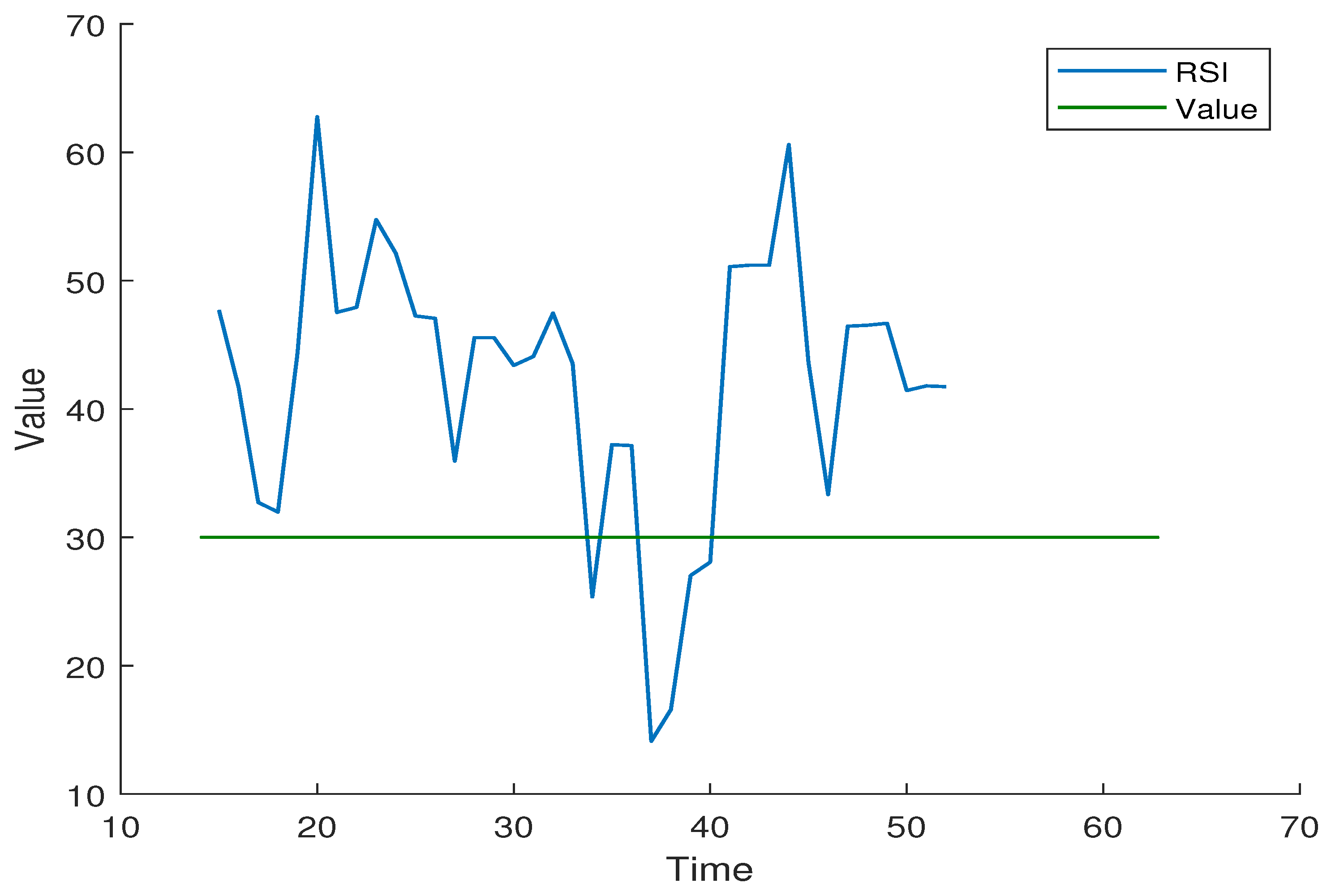
Figure 8 and Figure 9 present the daily return distribution of asset #10 and the relative strength index, respectively. Figure 9 displays the relative strength index. The stock has little risk if this index is below 30and should be bought. The stock has a lot of risk if this index reaches 70 and should be sold. After obtaining the optimal solution with the DEA-Mean-CVaR model, we found that the DEA-Mean-CVaR model suggested investing only in asset #10. By constructed the logarithmic return diagram of the proposed stock, we realized that the proposed stock was skewed to the right, which meant that there was a possibility of an increase in the return. Furthermore, by analyzing the relative strength index, we discovered that this asset had reached the number 30 and should be bought. Therefore, it can be concluded that in the first method, the model suggested an asset that should be bought according to the index and also, according to the histogram, there was a probability of a return from this stock.

The histogram of asset #3 return is shown in Figure 10. This asset received the most weight according to the Mean-CVaR model. The histogram illustrates that the return distribution of asset #3 exhibited kurtosis. Thus, there were extreme points (a sudden price increase) in this asset. Therefore, it can be inferred that the weights were assigned based on the momentary return in the Mean-CVaR model, whereas Figure 11 shows that the index has reached 70, so the stock risk is high and should be sold.

Table 8. The weight of each asset in automotive industry portfolios optimized with PSO and ICA algorithms under Mean-CVaR.

Asset ID	PSO Asset Weight			ICA Asset Weight
	90%	95%	99%	90%	95%	99%
1	0	0	0	0	0	0.0001
2	0	0	0.0007	0	0.0001	0.0001
3	0	0.0001	0.0504	0.0002	0.0003	0.0391
4	0.0661	0.0817	0.0806	0.0605	0.075	0.0796
5	0.1301	0.1143	0.0935	0.1325	0.1095	0.0942
6	0.0038	0.0736	0.0519	0.0096	0.0651	0.0488
7	0.0449	0.0566	0.0715	0.0414	0.0582	0.0762
8	0	0	0	0	0	0.0014
9	0.0843	0.0873	0.0421	0.0908	0.0884	0.0423
10	0.1539	0.1151	0.0597	0.1344	0.1095	0.0593
11	0.0386	0.0622	0.048	0.046	0.0515	0.0373
12	0.1303	0.0715	0.027	0.099	0.0655	0.0274
13	0.0009	0.0004	0.0248	0	0	0.0271
14	0.0339	0.0481	0.0422	0.0409	0.0443	0.042
15	0.0002	0	0.0424	0.0001	0.0001	0.0481
16	0.0937	0.0812	0.0918	0.0851	0.0832	0.0783
17	0.0119	0.0194	0.0333	0.0287	0.0207	0.0324
18	0.0008	0.0051	0.0404	0.0006	0.0125	0.0372
19	0.0333	0.0415	0.0137	0.0565	0.0436	0.0345
20	0.001	0.0108	0.0285	0.0011	0.0107	0.0355
21	0.1072	0.06	0.0549	0.0883	0.074	0.0563
22	0.0001	0	0.0591	0	0.0006	0.0597
23	0.0649	0.0707	0.0435	0.0784	0.0871	0.0433

, shows that both algorithms in levels 90 and 95 assigned the most weight to asset #10, with the highest expected return, and in level 99 they assigned the most weight to asset #5. Furthermore, according to

Table 9. Risk and return of optimized automotive industry portfolios.

Algorithm	Portfolio Return			Portfolio Risk
	90%	95%	99%	90%	95%	99%
Mean-CVaR-PSO	0.0031	0.003	0.0025	0.0562	0.0643	0.0663
Mean-CVaR-ICA	0.0031	0.003	0.0025	0.0538	0.0645	0.0657
Mean-CVaR	0.0033	0.0034	0.0034	0.0708	0.0994	0.1869

, the PSO algorithm under constant return showed more risk than the ICA algorithm.

Figure 12 shows that the frontier of the PSO algorithm was higher than that of the ICA algorithm, so the PSO portfolio under certain return conditions showed more returns than the ICA portfolio.

Table 10. Inputs and outputs, consisting of the risk (CVaR) and return of 15 stocksin a portfolio optimized with the ICA algorithm using the second method.

Portfolio	Input			Output
	ICA Portfolio Risk			ICA Portfolio Return
	90%	95%	99%	90%	95%	99%
1	0.037874	0.047221	0.063001	0.002127	0.002195	0.002177
2	0.037906	0.047277	0.063323	0.002113	0.002197	0.002173
3	0.037904	0.047251	0.063125	0.002124	0.002183	0.002216
4	0.037859	0.047265	0.062967	0.002104	0.002195	0.002149
5	0.037908	0.047194	0.063045	0.002121	0.002186	0.002186
6	0.037983	0.047194	0.063067	0.002142	0.002194	0.002211
7	0.037942	0.047294	0.063698	0.002144	0.002171	0.00217
8	0.03795	0.047352	0.063064	0.002131	0.002197	0.002223
9	0.039491	0.049404	0.068445	0.002392	0.002392	0.002394
10	0.043312	0.055871	0.081768	0.002675	0.002675	0.002675
11	0.050294	0.065357	0.104911	0.00296	0.002959	0.002959
12	0.0638	0.085905	0.113434	0.003243	0.003239	0.003063
13	0.064939	0.082137	0.094028	0.003277	0.003176	0.002892
14	0.057136	0.064369	0.065694	0.003154	0.002949	0.002459
15	0.053248	0.064454	0.065674	0.003084	0.002956	0.002457

and

Table 11. Inputs and outputs consisting of the risk (CVaR) and return of 15 stocks in a portfolio optimized with the PSO algorithm using the second method.

Portfolio	Input			Output
	PSO Portfolio Risk			PSO Portfolio Return
	90%	95%	99%	90%	95%	99%
1	0.037887	0.047152	0.062022	0.002122	0.002193	0.00225
2	0.037833	0.047148	0.06257	0.0021	0.002173	0.002238
3	0.03788	0.047137	0.062108	0.002095	0.002184	0.002243
4	0.037864	0.047155	0.061964	0.0021	0.002203	0.002223
5	0.037837	0.047133	0.063738	0.002087	0.002185	0.002125
6	0.037828	0.047152	0.062029	0.002098	0.002173	0.002213
7	0.037801	0.047148	0.062201	0.002096	0.002183	0.00221
8	0.037868	0.047143	0.063119	0.002111	0.002202	0.00216
9	0.039177	0.048741	0.064874	0.002392	0.002392	0.002392
10	0.043143	0.05426	0.079014	0.002675	0.002675	0.002677
11	0.049953	0.065218	0.098566	0.002959	0.00296	0.002964
12	0.065444	0.091678	0.146192	0.003244	0.003244	0.003177
13	0.058897	0.083458	0.109542	0.003161	0.003224	0.003068
14	0.063892	0.088723	0.098888	0.003258	0.00326	0.002992
15	0.056204	0.064258	0.064929	0.003147	0.002961	0.002465

show the inputs and outputs of the second method, including the CVaR of the portfolios in three levels of confidence, along with their returns. It was found that CVaR increased with increasing confidence levels.

As shown in

Table 12. Risk and return of stocks in an automotive industry portfolio optimized with the DEA-Mean-CVaR model.

Portfolio	Efficiency PSO Portfolio			Efficiency ICA Portfolio
	90%	95%	99%	90%	95%	99%
1	1	1	1	1	1	1
2	1	0.9998	0.9908	0.999	0.9986	0.9947
3	0.9994	1	0.9984	0.9991	0.9992	0.9979
4	1	1	1	1	1	1
5	0.9992	1	0.9722	0.9987	1	0.9988
6	0.9995	0.9997	0.9989	0.9967	1	0.9984
7	1	0.9998	0.9962	0.9978	0.9981	0.9885
8	1	1	0.9822	0.9983	0.9985	0.9988
9	1	1	0.9856	1	1	0.9298
10	1	1	0.9942	1	1	0.7894
11	1	1	0.9847	1	0.9732	0.6252
12	1	1	1	1	1	1
13	1	1	1	0.9127	0.8903	0.9051
14	1	1	1	1	1	1
15	1	1	1	1	0.9689	0.9963

, portfolios 1, 4, 12, and 14 were efficient in three levels for both algorithms. The number of efficient portfolios in three levels was higher in the PSO algorithm than in the ICA algorithm.Portfolio #15, which was considered as the output of the algorithms, was efficient in the PSO algorithm in three levels. After obtaining the numerical results, we tested our hypotheses using the Wilcoxon test.

According to

Table 13. Hypothesis test results.

Method	Mean	Std	Min	Max	Zval	Prob
(MCVaR)	0.0022	0.0003	0.0021	0.0034
(DEA-MCVaR)	0.0028	0.0005	0.0024	0.0040
(DEA-MCVaR)-(MCVaR)-Ret					−3.408	0.001
MCVaR-Rsk	0.2259	0.0267	0.1861	0.2695
MCVaR-PSO-Rsk	0.0582	0.0166	0.0471	0.0916
MCVaR-ICA-Rsk	0.0563	0.0133	0.0471	0.0859
(MCVaR-PSO)-(MCVaR)-Rsk					−3.408	0.001
(MCVaR-ICA)-(MCVaR)-Rsk					−3.408	0.001

, the probability was less than 0.05, so the hypothesis of return equality was rejected. In other words, there was a difference between the efficiencies. Furthermore, the hypothesis of risk equality was rejected because the probability was less than 0.05.

6. Discussion of Results

To interpret the results, we considered the confidence level of 95 and based our interpretations on the results obtained at the 95 levels. Focusing on the results, we found that when we extended the Mean-CVaR, the results were improved. The Mean-CVaR suggested that most investments should be on asset #3, but according to the RSI index, this asset reached 70 and should be sold because its risk was high. When we expanded the model to create a portfolio with efficient stocks, then solved it using the evolutionary algorithms PSO and ICA, we found that the stocks with the highest expected returns and which were efficient at three levels of risk were suggested by the two algorithms. The positive skewness of the daily return distribution of asset #10 showed that there was a possibility of an increase in returns for this stock in the future. The test of the first hypothesis informed us that there was a difference between the returns of the portfolios constructed using DEA-Mean-CVaR and Mean-CVaR. In other words, if the Mean-CVaR model was expanded, the investor would obtain more returns.The test of the second hypothesis showed that when we solved the Mean-CVaR model with evolutionary methods, the investment risk decreased because the algorithms tried to find the best solution. According to the return distribution and the RSI index and efficiency, asset #10 was the best answer, which was suggested by the two algorithms at the confidence level of 95. In the end, we found that the PSO portfolio’s efficient border is higher than the ICA portfolio’s efficient border and the number of efficient portfolios identified by the PSO algorithm was than that of the ICA algorithm. Therefore, this algorithm worked more successfully in portfolio optimization and offered better solutions.

7. Conclusions

In this research, we optimized an automotive industry portfolio for the Iranian stock market in two ways. These companies play an essential role in the Iranian stock market. At the beginning of the research, we proposed two hypotheses as follows: 1. The returns obtained in the DEA-Mean-CVaR portfolio were higher than the returns of the Mean-CVaR portfolio. 2. The use of the evolutionary methods PSO and ICA reduced the risk of the Mean-CVaR portfolio.

Then, we checked the price index of the automotive industry. Our focus on the the automotive group index showed that the distribution of the price index was skewed to the right, so it could be said that investing in the automotive market would bring returns. Therefore, with the help of 23 automotive companies, we formed a portfolio using two methods. In the first method, CVaR was formulated using DEA, and then this model was solved using the PSO algorithm and the ICA algorithm. Based on the results shown in Table 5, it was found that both algorithms led to the proposal to invest in assets that had the highest expected return and that were found to be efficient at three levels of confidenceand that should have been purchased according to the RSI index. Furthermore, considering Table 9, the risk and return of both algorithms were equal with three levels of confidence, so according to Figure 6, the frontiers of the two algorithms coincided. In the second method, was solved the CVaR model using the PSO and ICA algorithms, then evaluated the performance of the obtained securities. We found that out of 40 portfolios generated using the algorithms, only 15 portfolios were located at the border, and according to Table 12 of these 15 portfolios, only four portfolios in both algorithms were considered efficient at three levels.

The results of the testing of the hypotheses indicated that the development of the Mean-CVaR model increased returns, and the use of innovative methods in its solution reduced risk.

Similarly to [26], and as shown in Table 5 and Figure 6, we found that the development of portfolio selection models with the DEA model obtained better results.Furthermore, as shown in Table 12 and Figure 12, similarly to the research of [36,37], our results indicated that the PSO algorithm performed better in the task of portfolio optimization.

Finally, we conclude that when the Mean-CVaR model is developed using the DEA model and when evolutionary algorithms are used to the solution of these problems, we can invest more confidently in the proposed stocks. Overall, it can be stated that if investors have a low degree of risk aversion, they can take advantage of the combination of DEA and Mean-CVaR models. For future research, we suggested modeling other risk measures by means of DEA and then calculating solutions with the PSO algorithm to compare results with those the strength Pareto evolutionary algorithm.

References

1. Batrancea, L.; Rathnaswamy, M.K.; Batrancea, I. A Panel Data Analysis on Determinants of Economic Growth in Seven Non BCBS Countries. J. Knowl. Econ. 2021, 13, 1651–1665. [Google Scholar] [CrossRef]
2. Markowitz, H. Portfolio selection. J. Financ. 1952, 7, 77–91. [Google Scholar]
3. Linsmeier, T.J.; Pearson, N.D. Value at Risk. Financ. Anal. 2000, 56, 47–67. [Google Scholar] [CrossRef]
4. Rockafellar, R.T.; Uryasev, S. Optimization of Conditional Value at Risk. J. Risk 2020, 2, 21–41. [Google Scholar] [CrossRef]
5. Batrancea, L. An Econometric Approach Regarding the Impact of Fiscal Pressure on Equilibrium: Evidence from Electricity, Gas and Oil Companies Listed on the New York Stock Exchange. Mathematics 2021, 9, 630. [Google Scholar] [CrossRef]
6. Krokhmal, P.; Uryasev, S.; Palmquist, J. Portfolio Optimization with Conditional Value at Risk Objective and Constranints. J. Risk 2002, 4, 43–68. [Google Scholar] [CrossRef]
7. Bassett, G.W.; Koenker, R.; Kordas, G. Pessimistic portfolio allocation and Choquet expected. J. Financ. Econom. 2004, 2, 477–492. [Google Scholar]
8. Alexander, G.J.; Baptista, A.M. A comparison of VaR and CVaR constraints on portfolio selection with the mean-variance model. Manag. Sci. 2004, 50, 1261–1273. [Google Scholar] [CrossRef]
9. Huang, D.; Zhu, S.-S.; Fabozzi, F.J.; Fukushima, M. Portfolio selection with uncertain exit time:A robust cvar approach. J. Econ. Dyn. Control. 2008, 32, 594–623. [Google Scholar] [CrossRef]
10. Zhu, S.; Fukushima, M. Worst-case conditional value-at-risk with application to robust management. Oper. Res. 2009, 57, 1155–1168. [Google Scholar] [CrossRef]
11. Zhu, S.-S.; Fan, M.; Li, D. Portfolio management with robustness in both prediction and decision:A mixture model based learning approach. J. Econ. Dyn. Control. 2014, 48, 1–25. [Google Scholar] [CrossRef]
12. He, X.D.; Jiang, Z. Mean-Variance Portfolio Selection with Dynamic Targets for Expected Terminal Wealth. 2020. Available online: https://ssrn.com/abstract=3084657 (accessed on 23 November 2020).
13. Cui, X.; Gao, J.; Shi, Y.; Zhu, S. Time-consistent and self-coordination strategies for multiperiod mean-conditional value-at-risk portfolio selection. Eur. J. Oper. Res. 2019, 276, 781–789. [Google Scholar] [CrossRef]
14. Strub, M.S.; Li, D.; Cui, X.; Gao, J. Discrete-Time Mean-CVaR Portfolio Selection and Time-Consistency. J. Econ. Dyn. Control. 2019, 108, 103751. [Google Scholar] [CrossRef]
15. Benati, S.; Conde, E. A relative robust approach on expected returns with bounded CVaR for portfolio selection. Eur. J. Oper. Res. 2021, 296, 332–352. [Google Scholar] [CrossRef]
16. Aljinović, Z.; Marasović, B.; Šestanović, T. Cryptocurrency Portfolio Selection—A Multicriteria Approach. Mathematics 2021, 9, 1677. [Google Scholar] [CrossRef]
17. Bodnar, T.; Lindholm, M.; Niklasson, V.; Thorsén, E. Bayesian portfolio selection using VaR and CVaR. Appl. Math. Comput. 2022, 427, 127120. [Google Scholar] [CrossRef]
18. Gabrielli, P.; Aboutalebi, R.; Sansavini, G. Mitigating financial risk of corporate power purchase agreements via. Energy Econ. 2022, 109, 105980. [Google Scholar] [CrossRef]
19. Charnes, A.; Cooper, W.W.; Rhodes, E. Measuring the efficiency of decision making units. Eur. J. Oper. Res. 1987, 2, 429–444. [Google Scholar] [CrossRef]
20. Morey, M.R.; Morey, R.C. Mutual fund performance appraisals: A multi-horizon perspective with endogenous benchmarking. Omega 1999, 27, 241–258. [Google Scholar] [CrossRef]
21. Briec, W.; Kerstens, K.; Lesourd, J.B. Single Period Markowitz portfolio selection performance gauging and duality: A variation on the Luenberger shortage function. J. Optim. Theory Appl. 2004, 120, 1–27. [Google Scholar] [CrossRef]
22. Joro, T.; Na, P. Portfolio performance evaluation in a mean-variance-skowness framework. Eur. J. Oper. Res. 2006, 175, 446–461. [Google Scholar] [CrossRef]
23. Chen, Z.P.; Lin, R.Y. Mutual fund performance evaluation using data envelopment analysis with new risk measures. OR Spectr. 2006, 28, 375–398. [Google Scholar] [CrossRef]
24. Lamb, J.D.; Tee, K.-H. Data envelopment analysis models of investment funds. Eur. J. Oper. Res. 2012, 216, 687–696. [Google Scholar] [CrossRef]
25. Branda, M. Diversification-consistent data envelopment analysis with general deviation measures. Eur. J. Oper. Res. 2013, 226, 626–635. [Google Scholar] [CrossRef]
26. Mashayekhi, Z.; Omrani, H. An integrated multi-objective Markowitz–DEA cross-efficiency model with fuzzy returns for portfolio selection problem. Appl. Soft Comput. 2015, 38, 1–9. [Google Scholar] [CrossRef]
27. Zhang, Y.-J.; Chen, M.-Y. Evaluation the dynamic of performance of energy portfolio: Empirical evidence from the DEA directional distance function. Eur. J. Oper. Res. 2018, 269, 64–78. [Google Scholar] [CrossRef]
28. Amin, G.R.; Hajjami, M. Improving DEA Cross-efficiency optimization in portfolio selection. Expert Syst. Appl. 2021, 168, 114280. [Google Scholar] [CrossRef]
29. Xiao, H.; Ren, T.; Zhou, Z.; Liu, W. Parameter uncertainty in estimation of portfolio efficiency: Evidence from an interval diversification-consistent DEA approach. Omega 2021, 103, 102357. [Google Scholar] [CrossRef]
30. Zhou, Z.; Gao, M.; Xiao, H.; Wang, R.; Liu, W. Big data and portfolio optimization: A novel approach integrating DEA with multiple data sources. Omega 2021, 104, 102479. [Google Scholar] [CrossRef]
31. Kennedy, J.; Eberhart, R.C. Particle Swarm Optimization. Neural Netw. 1995, 4, 1942–1948. [Google Scholar]
32. Rehman, A.U.; Islam, A.; Belhaouari, S.B. Multi-Cluster Jumping Particle Swarm. IEEE Access 2020, 8, 189382–189394. [Google Scholar] [CrossRef]
33. Kassoul, K.; Belhaouari, S.B.; Cheikhrouhou, N. Dynamic Cognitive-Social Particle Swarm. In Proceedings of the 2021 7th International Conference on Automation, Robotics and Applications (ICARA), Prague, Czech Republic, 4–6 February 2021. [Google Scholar]
34. Cura, T. Partical swarm optimization approach to portfolio optimization. Nonlinear Anal. Real World Appl. 2009, 10, 2396–2406. [Google Scholar] [CrossRef]
35. Zhu, H.; Wang, Y.; Wang, K.; Chen, Y. Partical swarm optimization (PSO) for the constrained portfolio optimization problem. Expert Syst. Appl. 2011, 38, 10161–10169. [Google Scholar] [CrossRef]
36. Najafi, A.A.; Mushakhian, S. Multi-stage stochastic mean–semivariance–CVaR portfolio optimization under transaction costs. Appl. Math. Comput. 2015, 256, 445–458. [Google Scholar] [CrossRef]
37. Liu, C.; Yin, Y. Particle swarm optimised analysis of investment decision. Cogn. Syst. Res. 2018, 52, 685–690. [Google Scholar] [CrossRef]
38. Burney, S.M.; Jilani, T.; Tariq, H.; Amjad, U. A Portfolio Optimization Algorithm Using Fuzzy Granularity Based Clustering. Broad Res. Artifical Intell. Neurosci. 2019, 10, 159–173. [Google Scholar]
39. Kaucic, M. Equity portfolio managment with cardinality constraints and risk parity control using multi-objective particale swarm optimization. Comput. Oper. Res. 2019, 109, 300–316. [Google Scholar] [CrossRef]
40. Konstantinou, C.; Tzanetos, A.; Dounias, G. Cardinality constrained portfolio optimization with a hybrid scheme combining a Genetic Algorithm and Sonar Inspired Optimization. Oper. Res. 2020, 22, 2465–2487. [Google Scholar] [CrossRef]
41. Zhang, H. Optimization of risk control in financial markets based on particale swarm optimization algorithm. J. Comput. Appl. Math. 2020, 368, 112530. [Google Scholar] [CrossRef]
42. Atashpaz-Gargari, E.; Lucas, C. Imperialist Competitive Algorithm: An Algorithm for Optimization Inspired by Imperialistic Competition. In Proceedings of the 2007 IEEE Congress on Evolutionary Computation, Singapore, 25–28 September 2007; pp. 4661–4667. [Google Scholar]
43. Yin, Z.; Gao, Q. A Novel Imperialist Competitive Algorithm for Scheme Configuration Rules Extraction of Product Service. Procedia Cirp 2019, 80, 762–767. [Google Scholar] [CrossRef]
44. Saadatjoo, M.A.; Babamir, S.M. Test-data generation directed by program path coverage through imperialist competitive algorithm. Sci. Comput. Program. 2019, 184, 102304. [Google Scholar] [CrossRef]
45. Li, M.; Lei, D.; Cai, J. Two-level imperialist competitive algorithm for energy-efficient hybrid flow shop scheduling problem with relative importance of objectives. Swarm Evol. Comput. 2019, 49, 34–43. [Google Scholar] [CrossRef]
Figure 1. Particle updating process in PSO.
Mathematics 10 02808 g001
Figure 2. The departure of a colony to its relevant imperialist.
Mathematics 10 02808 g002
Figure 3. Normality test of price index.
Mathematics 10 02808 g003
Figure 4. Price index distribution.
Mathematics 10 02808 g004
Figure 5. Logarithmic return of each asset.
Mathematics 10 02808 g005
Figure 6. Frontiers of PSO and ICA algorithms using the first method.
Mathematics 10 02808 g006
Figure 7. Frontier of Mean-CVaR (%95).
Mathematics 10 02808 g007
Figure 8. Return distribution of asset #10.
Mathematics 10 02808 g008
Figure 9. Relative strength index of asset #10.
Mathematics 10 02808 g009
Figure 10. Return distribution of asset #3.
Mathematics 10 02808 g010
Figure 11. Relative strength index of asset #3.
Mathematics 10 02808 g011
Figure 12. Frontiers of PSO and ICA algorithms in the second method.
Mathematics 10 02808 g012