
SMoCo: A Powerful and Efficient Method Based on Self-Supervised Learning for Fault Diagnosis of Aero-Engine Bearing under Limited Data


Abstract
:1. Introduction
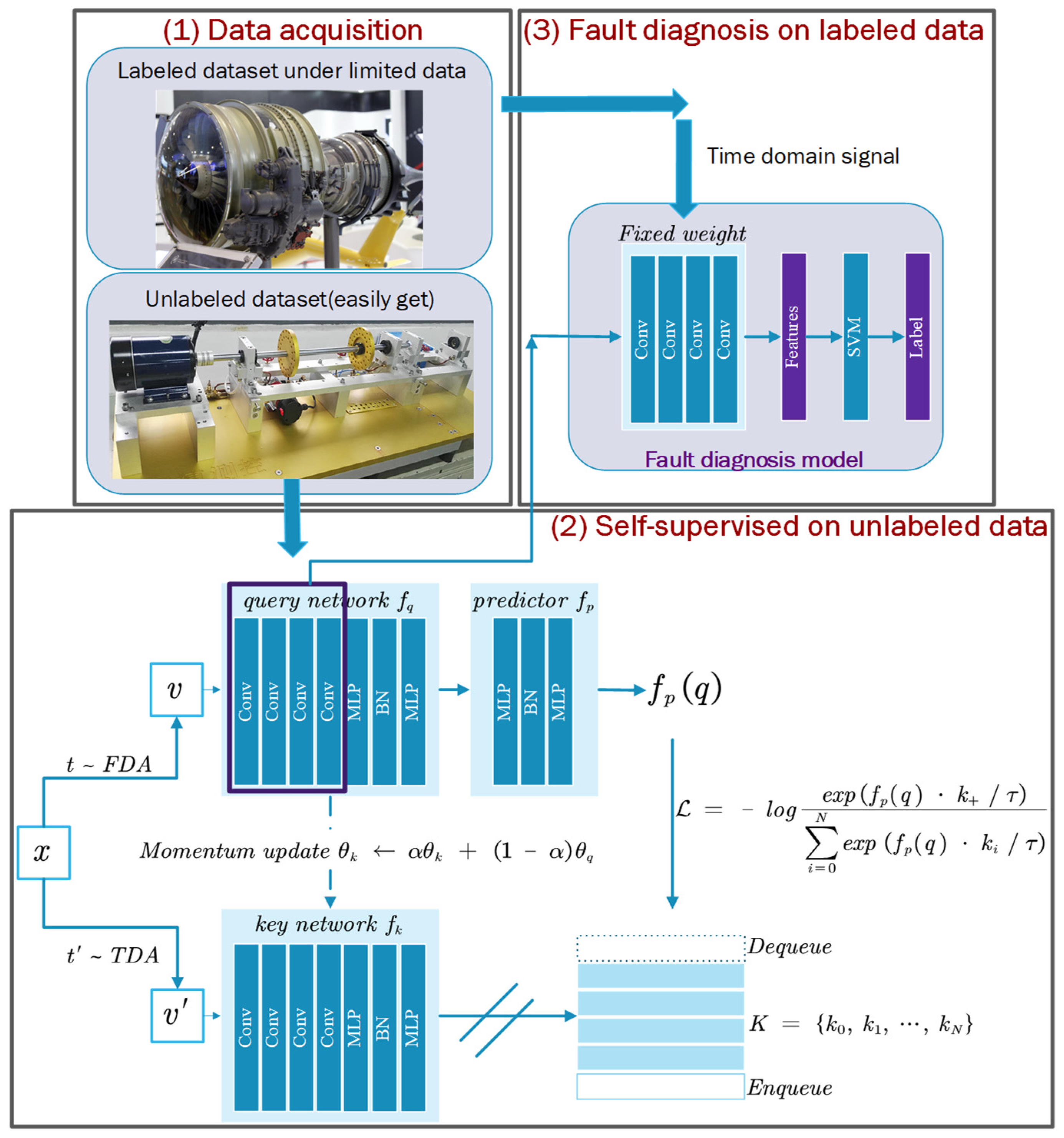
- In terms of structure, based on MoCo, this paper increases the performance of the model and the stability of training by introducing a predictor to the query network and adding batch normalization (BN) [26] to the multilayer perceptron (MLP) layer.
- In terms of data augmentation method, this paper proposes signal multimodal learning (SML), which enables the model to learn the signal representation from both the time domain and the frequency domain, thereby characterizing the signal from two dimensions.
- The unlabeled pre-training data used by SMoCo comes from a wide range of sources and is no longer limited to the same diagnostic object, which makes it more feasible in the real task.
- Experiments show that SMoCo can be used as a feature extractor with fixed weights to extract robust features after pre-training on artificially injected fault bearings, whether it is a bearing with different failure modes under different working conditions or a completely different type of rolling bearing. Aero-engine high-speed rolling bearings can achieve extremely high diagnostic accuracy with very few samples, providing timelier and more robust fault diagnosis than other state-of-the-art techniques.
- Further studies have shown that SMoCo can still achieve excellent performance with a much-reduced data volume and in the presence of strong noise, further broadening its applicability.
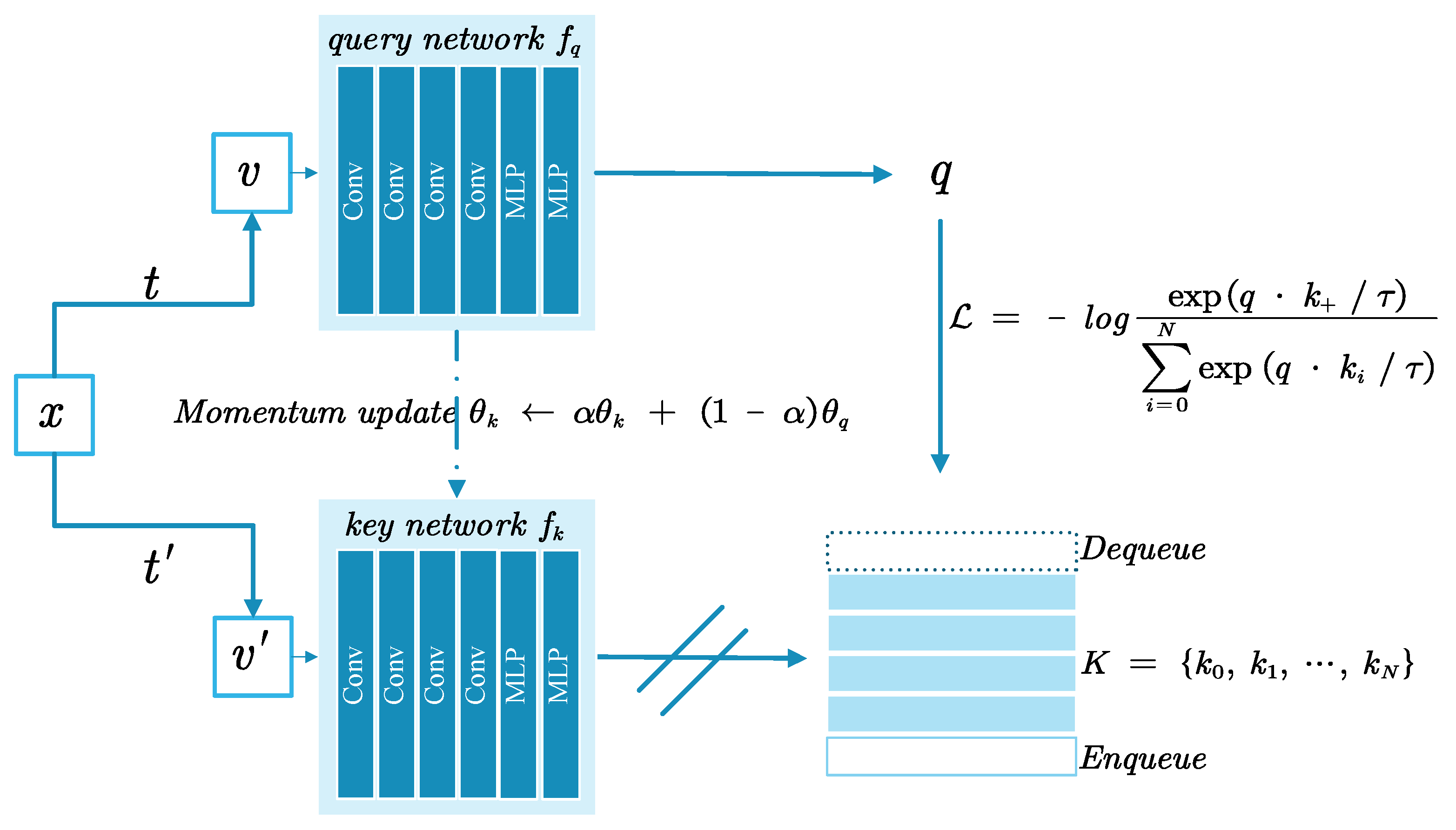
2. MoCo Network
3. SMoCo
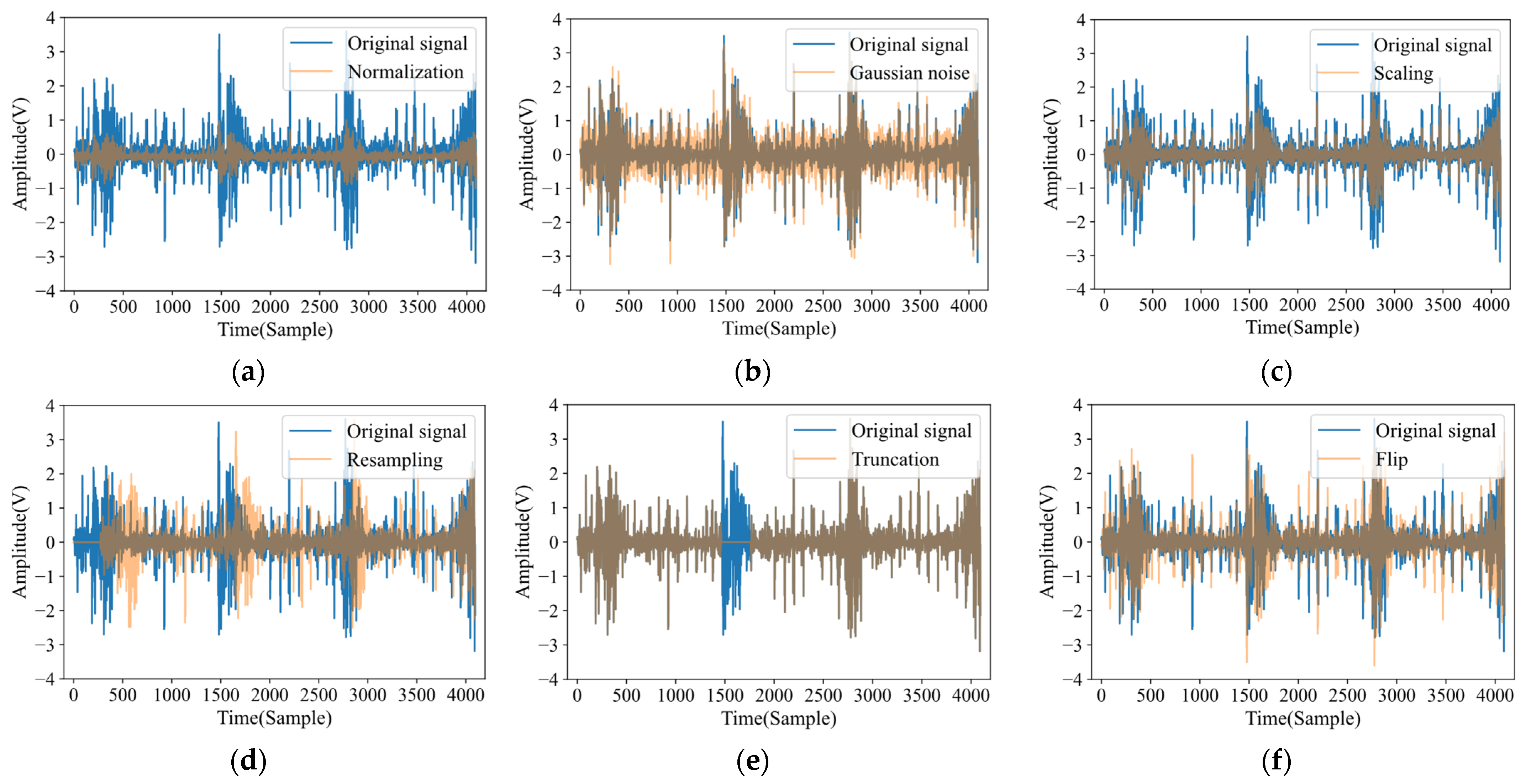
3.1. Signal Multimodal Learning (SML)
- Normalization: There are differences in the measurement range of different sensors. This strategy normalizes the signal to a uniform range, which is also beneficial for model training. The formula is as follows:
- Gaussian noise: There is an inevitable environmental noise problem during the operation of the device. This strategy adds Gaussian noise to the original signal to mimic this phenomenon. The formula is as follows:where n is generated by the Gaussian distribution .
- Scaling: This strategy increases the sensitivity of the model to signals of different amplitudes by directly amplifying or reducing the amplitude of the signal without losing the semantics contained in the original data. The formula is as follows:where s is generated from a Gaussian distribution .
- Resampling: This strategy improves the robustness of the model to variable speed scenarios by resampling and transforming the signal length to times the original length.
- Truncation: This strategy randomly covers part of the signal, and its formula is as follows:where is a binary sequence with subsequence zeros at random positions.
- Flip: The vibration signal usually vibrates up and down with 0 as the mean value. This strategy randomly flips the signal to increase the diversity of the signal. The formula is as follows:
3.2. Fault Diagnosis Based on SMoCo
| Algorithm 1. The detailed SMoCo. |
| Input: Structure of , , , temperature , momentum update , size batch size , learning rate , total number of optimization steps , distributions of transformations TDA, FDA, set of signals D Initialize parameters, , and for to do for do and and and end // Back-propagation // Momentum update without back-propagation // Update dictionary Enqueue and dequeue with and end Output: query network parameters |
4. Performance Verification of SMoCo
4.1. Self-Supervised on Artificially Damaged Bearing Data
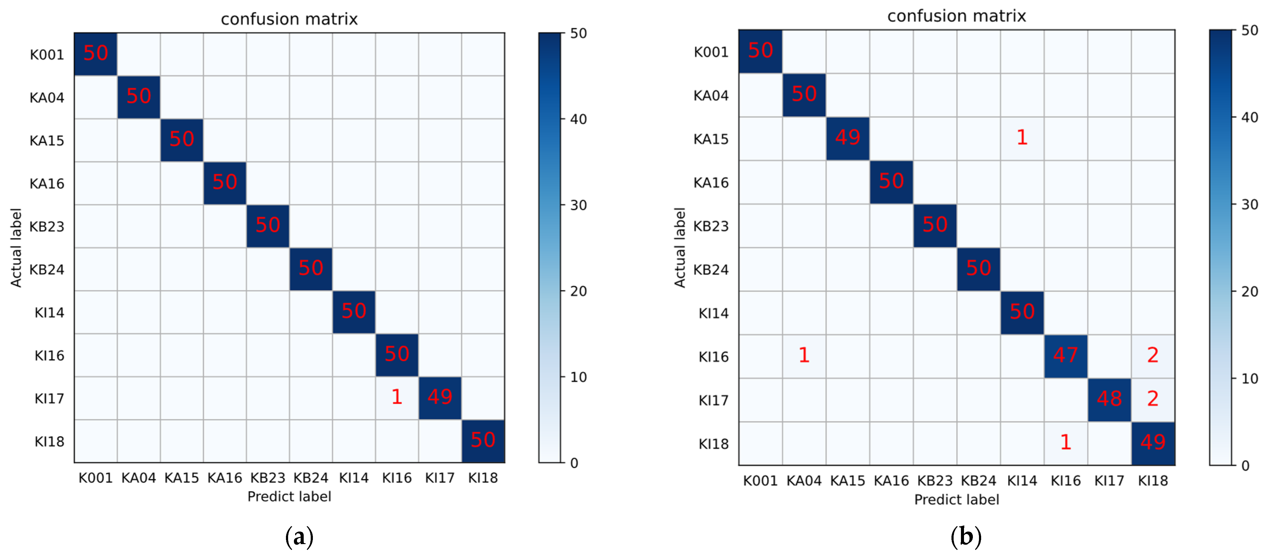
4.2. Fault Diagnosis on Same Products under Different Fault Characteristic Distributions
4.3. Fault Diagnosis on Different Products of Aero-Engine Bearing
5. Robustness Verification of SMoCo
5.1. Sensitivity to the Size of the Pre-Training Dataset
5.2. Sensitivity to Aero-Engine Bearing Dataset under Different Noise Levels
6. Conclusions
- In this paper, BN and a predictor are introduced to solve the deficiency of the MoCo structure, and SML is innovatively proposed according to the time domain and frequency domain of the signal, which regards the time-domain signal and frequency-domain signal as a positive pair. Therefore, a fault diagnosis method based on SMoCo is proposed.
- SMoCo uses easily available unlabeled data for self-supervised learning, the sources of which can be diverse and are not limited to objects that need to be diagnosed. Therefore, its acquisition range is wider, and its feasibility in practical diagnostic tasks is much greater than that of previous work.
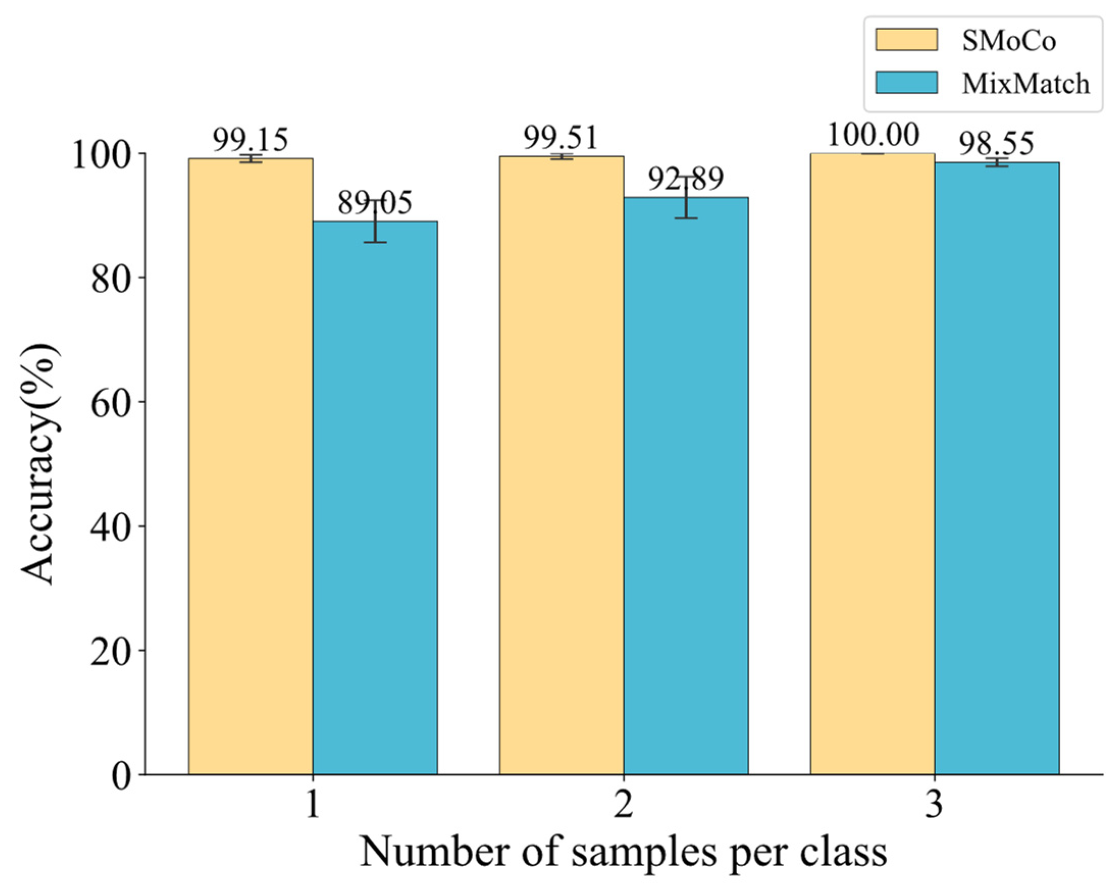
- This paper uses two independent bearing datasets from Paderborn University and the Polytechnic University of Turin for experimental verification. In the experiment, three important problems of aero-engine bearing fault diagnosis under the condition of limited data are studied, which are different working conditions, different failure modes, and different equipment. After SMoCo performs self-supervised learning on artificially injected faulted bearings, the trained feature extractor can be used to solve the above problems. The results show that the proposed SMoCo method can effectively solve the diagnosis problem in the case of limited data, it greatly exceeds the existing state-of-the-art methods both in accuracy and speed and is very little affected by limited data, even requiring only one sample per class to achieve high diagnostic accuracy for aero-engine bearing.
- Compared with representative methods, SMoCo still achieves good performance in the case of limited unlabeled pre-training data and less labeled training data with strong noise, demonstrating the robustness of SMoCo regarding data volume and noise.
Author Contributions
Funding
Institutional Review Board Statement
Informed Consent Statement
Data Availability Statement
Conflicts of Interest
References
- Wang, B.; Zhang, X.; Sun, C.; Chen, X. A Quantitative Intelligent Diagnosis Method for Early Weak Faults of Aviation High-Speed Bearings. ISA Trans. 2019, 93, 370–383. [Google Scholar] [CrossRef] [PubMed]
- Jiang, X.; Huang, Q.; Shen, C.; Wang, Q.; Xu, K.; Liu, J.; Shi, J.; Zhu, Z. Synchronous Chirp Mode Extraction: A Promising Tool for Fault Diagnosis of Rolling Element Bearings under Varying Speed Conditions. Chin. J. Aeronaut. 2022, 35, 348–364. [Google Scholar] [CrossRef]
- Wang, Y.; Tse, P.W.; Tang, B.; Qin, Y.; Deng, L.; Huang, T. Kurtogram Manifold Learning and Its Application to Rolling Bearing Weak Signal Detection. Measurement 2018, 127, 533–545. [Google Scholar] [CrossRef]
- Lei, Y.; Yang, B.; Jiang, X.; Jia, F.; Li, N.; Nandi, A.K. Applications of Machine Learning to Machine Fault Diagnosis: A Review and Roadmap. Mech. Syst. Signal Process. 2020, 138, 106587. [Google Scholar] [CrossRef]
- Feng, Y.; Chen, J.; Zhang, T.; He, S.; Xu, E.; Zhou, Z. Semi-Supervised Meta-Learning Networks with Squeeze-and-Excitation Attention for Few-Shot Fault Diagnosis. ISA Trans. 2022, 120, 383–401. [Google Scholar] [CrossRef] [PubMed]
- Yu, K.; Lin, T.R.; Ma, H.; Li, X.; Li, X. A Multi-Stage Semi-Supervised Learning Approach for Intelligent Fault Diagnosis of Rolling Bearing Using Data Augmentation and Metric Learning. Mech. Syst. Signal Process. 2021, 146, 107043. [Google Scholar] [CrossRef]
- Zhang, S.; Ye, F.; Wang, B.; Habetler, T.G. Semi-Supervised Bearing Fault Diagnosis and Classification Using Variational Autoencoder-Based Deep Generative Models. IEEE Sens. J. 2021, 21, 6476–6486. [Google Scholar] [CrossRef]
- Wen, L.; Gao, L.; Li, X. A New Deep Transfer Learning Based on Sparse Auto-Encoder for Fault Diagnosis. IEEE Trans. Syst. Man Cybern. Syst. 2019, 49, 136–144. [Google Scholar] [CrossRef]
- Wang, Y.; Sun, X.; Li, J.; Yang, Y. Intelligent Fault Diagnosis With Deep Adversarial Domain Adaptation. IEEE Trans. Instrum. Meas. 2021, 70, 3035385. [Google Scholar] [CrossRef]
- Zheng, H.; Wang, R.; Yang, Y.; Yin, J.; Li, Y.; Li, Y.; Xu, M. Cross-Domain Fault Diagnosis Using Knowledge Transfer Strategy: A Review. IEEE Access 2019, 7, 129260–129290. [Google Scholar] [CrossRef]
- Jing, L.; Tian, Y. Self-Supervised Visual Feature Learning With Deep Neural Networks: A Survey. IEEE Trans. Pattern Anal. Mach. Intell. 2021, 43, 4037–4058. [Google Scholar] [CrossRef]
- Zhang, R.; Isola, P.; Efros, A.A. Colorful Image Colorization. In Computer Vision–ECCV 2016; Leibe, B., Matas, J., Sebe, N., Welling, M., Eds.; Lecture Notes in Computer Science; Springer International Publishing: Cham, Switzerland, 2016; Volume 9907, pp. 649–666. ISBN 978-3-319-46486-2. [Google Scholar]
- Pathak, D.; Krähenbühl, P.; Donahue, J.; Darrell, T.; Efros, A.A. Context Encoders: Feature Learning by Inpainting. In Proceedings of the 2016 IEEE Conference on Computer Vision and Pattern Recognition (CVPR), Las Vegas, NV, USA, 27–30 June 2016; pp. 2536–2544. [Google Scholar]
- Noroozi, M.; Favaro, P. Unsupervised Learning of Visual Representations by Solving Jigsaw Puzzles. In Computer Vision–ECCV 2016; Leibe, B., Matas, J., Sebe, N., Welling, M., Eds.; Springer International Publishing: Cham, Switzerland, 2016; pp. 69–84. [Google Scholar]
- Ledig, C.; Theis, L.; Huszár, F.; Caballero, J.; Cunningham, A.; Acosta, A.; Aitken, A.; Tejani, A.; Totz, J.; Wang, Z.; et al. Photo-Realistic Single Image Super-Resolution Using a Generative Adversarial Network. In Proceedings of the 2017 IEEE Conference on Computer Vision and Pattern Recognition (CVPR), Honolulu, HI, USA, 21–26 July 2017; pp. 105–114. [Google Scholar]
- Wang, H.; Liu, Z.; Ge, Y.; Peng, D. Self-Supervised Signal Representation Learning for Machinery Fault Diagnosis under Limited Annotation Data. Knowl. Based Syst. 2022, 239, 107978. [Google Scholar] [CrossRef]
- Tian, Y.; Sun, C.; Poole, B.; Krishnan, D.; Schmid, C.; Isola, P. What Makes for Good Views for Contrastive Learning? In Advances in Neural Information Processing Systems; Curran Associates, Inc.: New York, NY, USA, 2020; Volume 33, pp. 6827–6839. [Google Scholar]
- Chen, T.; Kornblith, S.; Norouzi, M.; Hinton, G. A Simple Framework for Contrastive Learning of Visual Representations. In Proceedings of the 37th International Conference on Machine Learning, PMLR, Vienna, Austria, 21 November 2020; pp. 1597–1607. [Google Scholar]
- Chen, T.; Kornblith, S.; Swersky, K.; Norouzi, M.; Hinton, G.E. Big Self-Supervised Models Are Strong Semi-Supervised Learners. In Advances in Neural Information Processing Systems; Curran Associates, Inc.: New York, NY, USA, 2020; Volume 33, pp. 22243–22255. [Google Scholar]
- Caron, M.; Misra, I.; Mairal, J.; Goyal, P.; Bojanowski, P.; Joulin, A. Unsupervised Learning of Visual Features by Contrasting Cluster Assignments. In Advances in Neural Information Processing Systems; Curran Associates, Inc.: New York, NY, USA, 2020; Volume 33, pp. 9912–9924. [Google Scholar]
- Grill, J.-B.; Strub, F.; Altché, F.; Tallec, C.; Richemond, P.H.; Buchatskaya, E.; Doersch, C.; Pires, B.A.; Guo, Z.D.; Azar, M.G.; et al. Bootstrap Your Own Latent: A New Approach to Self-Supervised Learning. Adv. Neural Inf. Processing Syst. 2020, 33, 21271–21284. [Google Scholar]
- Wei, M.; Liu, Y.; Zhang, T.; Wang, Z.; Zhu, J. Fault Diagnosis of Rotating Machinery Based on Improved Self-Supervised Learning Method and Very Few Labeled Samples. Sensors 2021, 22, 192. [Google Scholar] [CrossRef]
- Ding, Y.; Zhuang, J.; Ding, P.; Jia, M. Self-Supervised Pretraining via Contrast Learning for Intelligent Incipient Fault Detection of Bearings. Reliab. Eng. Syst. Saf. 2022, 218, 108126. [Google Scholar] [CrossRef]
- He, K.; Fan, H.; Wu, Y.; Xie, S.; Girshick, R. Momentum Contrast for Unsupervised Visual Representation Learning. In Proceedings of the 2020 IEEE/CVF Conference on Computer Vision and Pattern Recognition (CVPR), Seattle, WA, USA, 13–19 June 2020. [Google Scholar]
- Peng, T.; Shen, C.; Sun, S.; Wang, D. Fault Feature Extractor Based on Bootstrap Your Own Latent and Data Augmentation Algorithm for Unlabeled Vibration Signals. IEEE Trans. Ind. Electron. 2022, 69, 9547–9555. [Google Scholar] [CrossRef]
- Ioffe, S.; Szegedy, C. Batch Normalization: Accelerating Deep Network Training by Reducing Internal Covariate Shift. arXiv 2015, arXiv:1502.03167. [Google Scholar]
- Oord, A.; van den Li, Y.; Vinyals, O. Representation Learning with Contrastive Predictive Coding. arXiv 2018, arXiv:1807.03748. [Google Scholar]
- Lessmeier, C.; Kimotho, J.K.; Zimmer, D.; Sextro, W. Condition Monitoring of Bearing Damage in Electromechanical Drive Systems by Using Motor Current Signals of Electric Motors: A Benchmark Data Set for Data-Driven Classification. In Proceedings of the PHM Society European Conference, Bilbao, Spain, 5–8 July 2016; Volume 3. [Google Scholar] [CrossRef]
- Zhao, Z.; Li, T.; Wu, J.; Sun, C.; Wang, S.; Yan, R.; Chen, X. Deep Learning Algorithms for Rotating Machinery Intelligent Diagnosis: An Open Source Benchmark Study. ISA Trans. 2020, 107, 224–255. [Google Scholar] [CrossRef]
- He, K.; Zhang, X.; Ren, S.; Sun, J. Deep Residual Learning for Image Recognition. In Proceedings of the 2016 IEEE Conference on Computer Vision and Pattern Recognition (CVPR), Las Vegas, NV, USA, 27–30 June 2016; pp. 770–778. [Google Scholar]
- Berthelot, D.; Carlini, N.; Goodfellow, I.; Papernot, N.; Oliver, A.; Raffel, C.A. MixMatch: A Holistic Approach to Semi-Supervised Learning. In Advances in Neural Information Processing Systems; Curran Associates, Inc.: New York, NY, USA, 2019; Volume 32. [Google Scholar]
- Daga, A.P.; Fasana, A.; Marchesiello, S.; Garibaldi, L. The Politecnico Di Torino Rolling Bearing Test Rig: Description and Analysis of Open Access Data. Mech. Syst. Signal Process. 2019, 120, 252–273. [Google Scholar] [CrossRef]
- Forouzanfar, M.; Safaeipour, H.; Casavola, A. Oscillatory Failure Case Detection in Flight Control Systems via Wavelets Decomposition. In ISA Transactions; Elsevier: Amsterdam, The Netherlands, 2021. [Google Scholar] [CrossRef]
- Safaeipour, H.; Forouzanfar, M.; Ramezani, A. Incipient Fault Detection in Nonlinear Non-Gaussian Noisy Environment. Measurement 2021, 174, 109008. [Google Scholar] [CrossRef]
- Ortiz Ortiz, F.J.; Rodríguez-Ramos, A.; Llanes-Santiago, O. A Robust Fault Diagnosis Method in Presence of Noise and Missing Information for Industrial Plants. In Proceedings of the Pattern Recognition; Springer International Publishing: Cham, Switzerland, 2022; pp. 35–45. [Google Scholar]
- Fang, H.; Deng, J.; Bai, Y.; Feng, B.; Li, S.; Shao, S.; Chen, D. CLFormer: A Lightweight Transformer Based on Convolutional Embedding and Linear Self-Attention With Strong Robustness for Bearing Fault Diagnosis Under Limited Sample Conditions. IEEE Trans. Instrum. Meas. 2022, 71, 3132327. [Google Scholar] [CrossRef]


| Name of Setting | Rotational Speed [rpm] | Load Torque [Nm] | Radial Force [N] |
|---|---|---|---|
| N09_M07_F10 | 900 | 0.7 | 1000 |
| N15_M07_F10 | 1500 | 0.7 | 1000 |
| N15_M01_F10 | 1500 | 0.1 | 1000 |
| N15_M07_F04 | 1500 | 0.7 | 400 |
| Bearing Code | Damaged Element | Damaged Extent | Damage Method |
|---|---|---|---|
| K001 | Health state | / | Run-in 50 h before test |
| KA01 | Outer ring | Level 1 | Made by EDM |
| KA03 | Outer ring | Level 2 | Made by electric engraver |
| KA05 | Outer ring | Level 1 | Made by electric engraver |
| KA06 | Outer ring | Level 2 | Made by electric engraver |
| KA07 | Outer ring | Level 1 | Made by drilling |
| KA08 | Outer ring | Level 2 | Made by drilling |
| KA09 | Outer ring | Level 2 | Made by drilling |
| KI01 | Inner ring | Level 1 | Made by EDM |
| KI03 | Inner ring | Level 1 | Made by electric engraver |
| KI05 | Inner ring | Level 1 | Made by electric engraver |
| KI07 | Inner ring | Level 2 | Made by electric engraver |
| KI08 | Inner ring | Level 2 | Made by electric engraver |
| Hyperparameter | Value | Data Augmentation | Value |
|---|---|---|---|
| Batch size | 64 | Normalization | / |
| Optimizer | SGD | Gaussian noise | |
| Learning rate | 0.1 | Scaling | |
| Momentum | 0.9 | Resampling | |
| Weight decay | 0.0001 | Truncation | Truncation length = 100 |
| Epochs | 350 | Flip | / |
| Learning rate schedule | Cosine | ||
| Queue size | 65536 | ||
| Momentum update | 0.999 | ||
| Temperature | 0.07 |
| Bearing Code | Damaged Element | Fault Mode | Damage Form | Arrangement | Damaged Extent |
|---|---|---|---|---|---|
| K001 | Health state | / | / | / | / |
| KA04 | Outer ring | Fatigue: pitting | Single damage | No repetition | Level 1 |
| KA15 | Outer ring | Plastic deform: Indentations | Single damage | No repetition | Level 1 |
| KA16 | Outer ring | Fatigue: pitting | Repetitive damage | Random | Level 2 |
| KB23 | Outer ring and inner ring | Fatigue: pitting | Multiple damage | Random | Level 2 |
| KB24 | Outer ring and inner ring | Fatigue: pitting | Multiple damage | No repetition | Level 3 |
| KI14 | Outer ring | Fatigue: pitting | Multiple damage | No repetition | Level 1 |
| KI16 | Outer ring | Fatigue: pitting | Single damage | No repetition | Level 3 |
| KI17 | Inner ring | Fatigue: pitting | Repetitive damage | Random | Level 1 |
| KI18 | Inner ring | Fatigue: pitting | Single damage | No repetition | Level 2 |
| Method | Accuracy (%) | Time (s) |
|---|---|---|
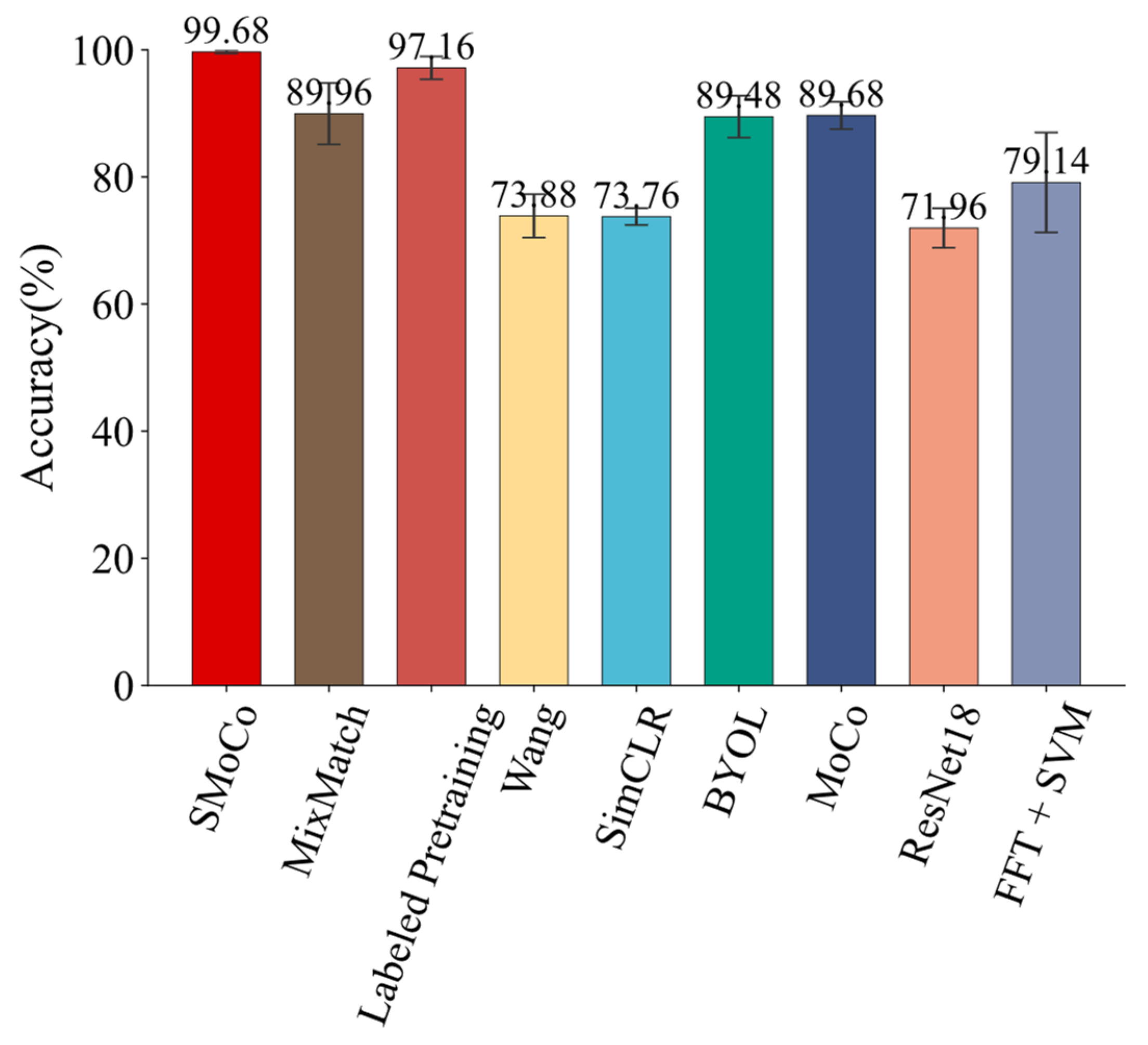
| SMoCo | 99.68 ± 0.26 | 1.47 |
| MixMatch | 89.96 ± 4.84 | 411.24 |
| Labeled Pretraining | 97.16 ± 1.80 | 25.11 |
| Wang | 73.88 ± 3.40 | 29.93 |
| SimCLR | 73.76 ± 1.35 | 30.44 |
| BYOL | 89.48 ± 3.29 | 30.72 |
| MoCo | 89.68 ± 2.16 | 30.75 |
| ResNet18 | 71.96 ± 3.13 | 26.26 |
| FFT + SVM | 79.14 ± 7.86 | 0.16 |
| Damaged Element | Diameter (μm) | Fault Mode Rotation Speed (r/min) | Load (N) | Training Samples | Testing Samples | Label |
|---|---|---|---|---|---|---|
| Healthy | / | 24,000 | 1400 | 3 | 50 | 0 |
| Inner ring | 450 | 24,000 | 1400 | 3 | 50 | 1 |
| Inner ring | 250 | 24,000 | 1400 | 3 | 50 | 2 |
| Inner ring | 150 | 24,000 | 1400 | 3 | 50 | 3 |
| Roller | 450 | 24,000 | 1400 | 3 | 50 | 4 |
| Roller | 250 | 24,000 | 1400 | 3 | 50 | 5 |
| Roller | 150 | 24,000 | 1400 | 3 | 50 | 6 |
| Inner ring | 450 | 18,000 | 1400 | 3 | 50 | 7 |
| Inner ring | 250 | 18,000 | 1400 | 3 | 50 | 8 |
| Inner ring | 150 | 18,000 | 1400 | 3 | 50 | 9 |
| Roller | 450 | 18,000 | 1400 | 3 | 50 | 10 |
| Roller | 250 | 18,000 | 1400 | 3 | 50 | 11 |
| Roller | 150 | 18,000 | 1400 | 3 | 50 | 12 |
| Method | Accuracy (%) | Time (s) |
|---|---|---|
| SMoCo | 100.00 ± 0.00 | 1.60 |
| MixMatch | 98.55 ± 0.65 | 469.06 |
| Labeled Pretraining | 90.92 ± 2.11 | 30.62 |
| Wang | 74.65 ± 4.56 | 36.04 |
| SimCLR | 81.85 ± 4.06 | 37.32 |
| BYOL | 85.66 ± 2.82 | 35.12 |
| MoCo | 84.00 ± 4.10 | 40.42 |
| ResNet18 | 82.83 ± 2.88 | 29.78 |
| FFT + SVM | 94.94 ± 4.19 | 0.15 |
| Method | Number of Samples Per Class on Dataset 2 | ||||
|---|---|---|---|---|---|
| 1 (F1/%) | 2 (F1/%) | 3 (F1/%) | 4 (F1/%) | 5 (F1/%) | |
| SMoCo + 2000 | 94.39 | 97.86 | 98.92 | 99.60 | 99.64 |
| SMoCo + 1500 | 92.35 | 95.43 | 97.79 | 98.52 | 98.76 |
| SMoCo + 1000 | 91.80 | 94.90 | 96.76 | 98.07 | 98.51 |
| SMoCo + 500 | 89.85 | 94.26 | 96.46 | 97.00 | 97.95 |
| SMoCo + 100 | 89.33 | 94.19 | 96.26 | 96.65 | 97.61 |
| Labeled Pretraining + 2000 | 88.33 | 94.24 | 96.20 | 96.84 | 97.20 |
| Method | Number of Samples Per Class on Dataset 3 | ||
|---|---|---|---|
| 1 (F1/%) | 2 (F1/%) | 3 (F1/%) | |
| SMoCo + 2000 | 99.46 | 99.84 | 99.94 |
| SMoCo + 1500 | 98.31 | 99.11 | 99.54 |
| SMoCo + 1000 | 98.01 | 99.04 | 99.38 |
| SMoCo + 500 | 97.74 | 98.86 | 99.20 |
| SMoCo + 100 | 97.04 | 98.21 | 98.89 |
| MixMatch + 2000 | 88.51 | 94.27 | 97.43 |
| Method | SNR | ||||||||||
|---|---|---|---|---|---|---|---|---|---|---|---|
| 0 dB | 1 dB | 2 dB | 3 dB | 4 dB | 5 dB | 6 dB | 7 dB | 8 dB | 9 dB | 10 dB | |
| SMoCo + 3 | 96.61 | 97.60 | 97.90 | 98.03 | 98.65 | 98.74 | 99.23 | 99.53 | 99.56 | 99.69 | 99.75 |
| SMoCo + 2 | 95.50 | 95.61 | 96.64 | 97.63 | 98.00 | 98.15 | 98.43 | 98.98 | 99.10 | 99.29 | 99.35 |
| SMoCo + 1 | 91.54 | 92.03 | 92.74 | 93.75 | 94.92 | 96.06 | 96.68 | 97.08 | 97.32 | 97.93 | 98.58 |
| MixMatch | 54.84 | 67.54 | 72.41 | 79.27 | 85.79 | 90.95 | 92.94 | 93.56 | 93.72 | 94.99 | 95.58 |
| FFT + SVM | 83.28 | 85.46 | 87.15 | 88.55 | 89.98 | 90.85 | 91.41 | 91.95 | 92.89 | 93.11 | 94.09 |
Publisher’s Note: MDPI stays neutral with regard to jurisdictional claims in published maps and institutional affiliations. |
© 2022 by the authors. Licensee MDPI, Basel, Switzerland. This article is an open access article distributed under the terms and conditions of the Creative Commons Attribution (CC BY) license (https://creativecommons.org/licenses/by/4.0/).
Share and Cite
Yan, Z.; Liu, H. SMoCo: A Powerful and Efficient Method Based on Self-Supervised Learning for Fault Diagnosis of Aero-Engine Bearing under Limited Data. Mathematics 2022, 10, 2796. https://doi.org/10.3390/math10152796
Yan Z, Liu H. SMoCo: A Powerful and Efficient Method Based on Self-Supervised Learning for Fault Diagnosis of Aero-Engine Bearing under Limited Data. Mathematics. 2022; 10(15):2796. https://doi.org/10.3390/math10152796
Chicago/Turabian StyleYan, Zitong, and Hongmei Liu. 2022. "SMoCo: A Powerful and Efficient Method Based on Self-Supervised Learning for Fault Diagnosis of Aero-Engine Bearing under Limited Data" Mathematics 10, no. 15: 2796. https://doi.org/10.3390/math10152796