Article

Graph Burning: Mathematical Formulations and Optimal Solutions

by
Jesús García-Díaz
1,2,*,
Lil María Xibai Rodríguez-Henríquez
1,2,
Julio César Pérez-Sansalvador
1,2 and
Saúl Eduardo Pomares-Hernández
2,3
1
Consejo Nacional de Ciencia y Tecnología, Mexico City 03940, Mexico
2
Instituto Nacional de Astrofísica, Óptica y Electrónica, Coordinación de Ciencias Computacionales, Puebla 72840, Mexico
3
Laboratoire d’Analyse et d’Architecture des Aystèmes du Centre National de la Recherche Scientifique (LAAS-CNRS), Université de Toulouse, INSA, F-31400 Toulouse, France
*
Author to whom correspondence should be addressed.
Mathematics 2022, 10(15), 2777; https://doi.org/10.3390/math10152777
Submission received: 4 February 2022 / Revised: 28 July 2022 / Accepted: 1 August 2022 / Published: 5 August 2022
(This article belongs to the Section Network Science)

Abstract

:
The graph burning problem is an NP-hard combinatorial optimization problem that helps quantify how vulnerable a graph is to contagion. This paper introduces three mathematical formulations of the problem: an integer linear program (ILP) and two constraint satisfaction problems (CSP1 and CSP2). Thanks to off-the-shelf optimization software, these formulations can be solved optimally over arbitrary graphs; this is relevant because the only algorithms designed to date for this problem are approximation algorithms and heuristics, which do not guarantee to find optimal solutions. We empirically compared the proposed formulations using random graphs and off-the-shelf optimization software. The results show that CSP1 and CSP2 tend to reach optimal solutions in less time than the ILP. Therefore, we executed them over some benchmark graphs of order at most 5908. The previously best-known solutions for some of these graphs were improved. We draw some empirical observations from the experimental results. For instance, we find the tendency: the larger the graph’s optimal solution, the more difficult it is to find it. Finally, the resulting set of optimal solutions might be helpful as a benchmark dataset for the performance evaluation of non-exact algorithms.

1. Introduction

The graph burning problem (GBP) is an NP-hard combinatorial optimization problem introduced in 2014 in the context of social contagion [1]. This problem, concerned with the sequential spread of information over a graph, considers that information can be spread from different places and times [1,2]. In this paper, by graph we refer to an undirected simple graph [3]. Computer network message propagation is an example of a real-world problem that the GBP may model; in this scenario, an initial spreading entity can send a message one host at a time, while these hosts can propagate the message only to their neighbors [4,5]. The GBP may model other real-world problems: social contagion in social networks and the spread of viral infections under a very idealistic context [1,6].
The GBP receives a graph G = ( V , E ) as input, and its goal is to find a minimum length sequence of vertices ( s 1 , s 2 , , s k ) that burns all graph’s vertices by following the burning process. This process consists of repeating the following steps from i = 1 to k, where all vertices are unburned at the beginning, and once a vertex is burned, it remains in that state.
a
The neighbors of the burned vertices get burned.
b
Vertex s i gets burned.
Any sequence that burns all the vertices of the input graph by following the burning process is known as a burning sequence. Thus, the GBP seeks a burning sequence of minimum length; this length is known as the burning number and is denoted by b ( G ) [1,2]. 
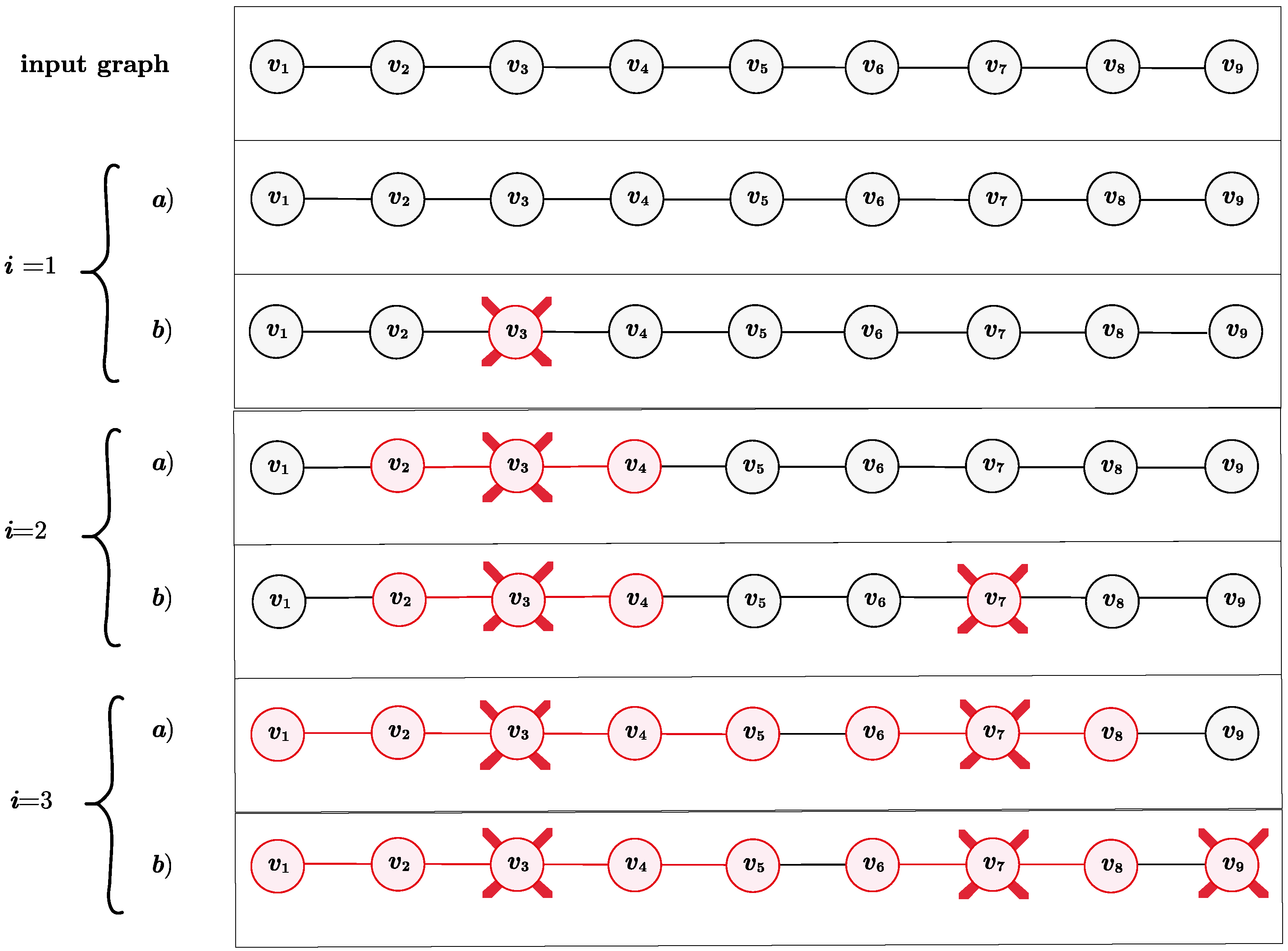
Figure 1 shows the execution of the burning process over a nine vertices path with optimal burning sequence ( v 3 , v 7 , v 9 ) . Certainly, this example is very simple. Thus, for further clarification, 
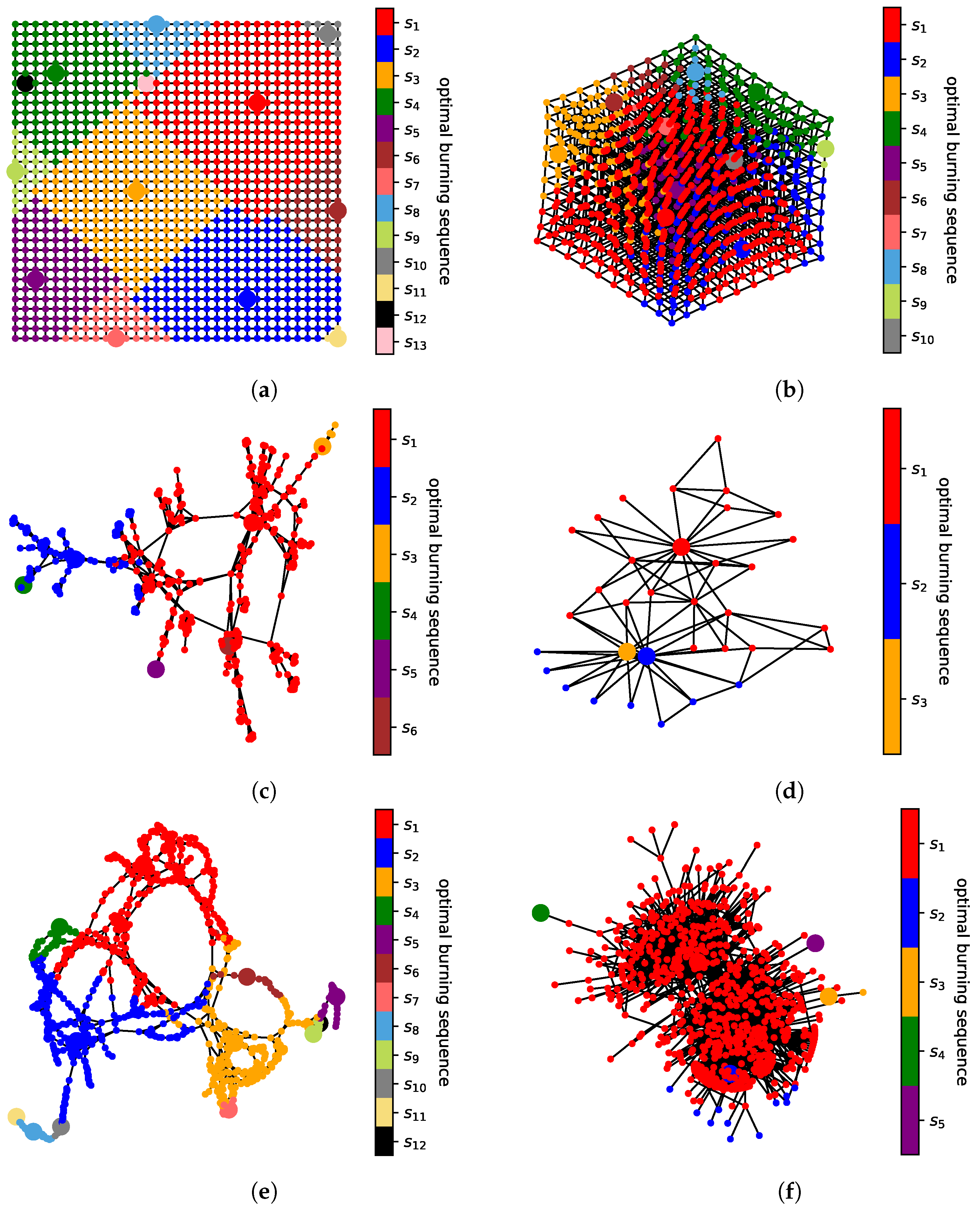
Figure 2 shows the optimal burning sequence of more interesting graphs. These optimal solutions were computed using the proposed mathematical formulations, which are introduced in Section 3. In all these graphs, the bigger vertices are elements s i of the burning sequence, and the color assigned to each vertex is the color of the vertex s i with the smaller index that burns it.
Due to its NP-hard nature, the GBP has been approached chiefly through approximation algorithms and heuristics. Some of these proposals are based on centrality measures and binary search over the possible values of the burning number b ( G ) . According to experimental results, these heuristics and approximation algorithms have an acceptable performance [4,5,6,7,8]. However, they do not guarantee to find optimal solutions. Therefore, there is a need for a mechanism for finding optimal solutions for arbitrary graphs. One of these mechanisms is mathematical formulations, which can be solved using off-the-shelf optimization software. For this reason, this paper introduces three novel mathematical formulations for the GBP: an integer linear program (ILP) and two constraint satisfaction problems (CSP1 and CSP2). Given the NP-hard nature of the problem, solving these formulations can take exponential time. Therefore, there must be a limit to their practicality. Through experimentation, we estimated such a limit.
The remaining part of the paper is organized as follows. Section 2 presents the background of the problem and the main definitions used in this document. Section 3 introduces the proposed mathematical formulations. Section 4 presents an empirical performance comparison among these formulations using random graphs and off-the-shelf optimization software. Section 5 reports optimal solutions found by the implemented CSP1 and CSP2 over some synthetic and real-world graphs using off-the-shelf optimization software. Finally, Section 6 presents the concluding remarks.

2. Background

Let us begin by listing some basic definitions used throughout the paper. Observe that a graph is often called an undirected simple graph to distinguish it from directed graphs and multigraphs; however, in this paper, we only use the word graph to refer to this mathematical object.
Definition 1.
Subsets with k elements are known as k-element subsets [3].
Definition 2.
A graph G = ( V , E ) is an ordered pair consisting of a set of vertices V and a set of edges E, where E contains 2-element subsets of V. The vertices and edges of any given graph J are also represented by V ( J ) and E ( J ) , respectively [3].
Definition 3.
Given a graph G = ( V , E ) , the distance d ( u , v ) between vertices u , v V is defined as the number of edges in their shortest path.
Definition 4.
Given a graph G = ( V , E ) , the open neighborhood N ( v ) of a vertex v V is the set of vertices at distance one from v. Notice that v N ( v ) .
Definition 5.
Given a graph G = ( V , E ) , the closed neighborhood N [ v ] of a vertex v V is the set of vertices at distance at most one from v. In other words, N [ v ] = N ( v ) { v } .
Definition 6.
Given a graph G = ( V , E ) , the closed k t h neighborhood N k [ v ] of a vertex v V is the set of vertices at distance at most k from v. Notice that N 0 [ v ] = { v } and N 1 [ v ] = N [ v ] .
Definition 7.
A finite sequence with no repeated elements is a bijective function
f : S { x Z + | x | S | } ,
where S is the set of objects in the sequence and | S | is its length. Notice that f ( v ) is v’s position in the sequence and that each object in S is assigned to exactly one position.
The decision version of the GBP is NP-complete. This problem receives as input a graph G = ( V , E ) and a positive integer k; it asks if a burning sequence of length at most k exists. The problem remains NP-complete when restricted to trees of maximum degree three, chordal graphs, bipartite graphs, planar graphs, spider graphs, and disconnected graphs [2]. The optimization version of the problem also remains NP-hard for trees and graphs with disjoint paths [7]. Regarding arbitrary graphs, two approximation algorithms are reported in the literature; they have an approximation factor of 3 and 3 2 / b ( G ) , respectively [7,8]. There is a 2-approximation algorithm for trees, a 1.5-approximation algorithm for graphs with disjoint paths, and a 2-approximation algorithm for square grids [6,7]. For minimization problems, a ρ -approximation algorithm returns solutions of size at most ρ · O P T , where O P T is the size of the optimal solution and ρ 1 . In the case of maximization problems, a ρ -approximation algorithm returns solutions of size at least ( 1 / ρ ) · O P T [9]. Besides approximation algorithms, some heuristics have been proposed too [4,5]; these are mainly based on centrality measures and binary search over the set of possible values of b ( G ) .
The GBP has been approached mostly from a theoretical point of view. As a result, many of its properties over specific graph families have been identified. Among these families are paths [2,7], trees [2,7], grids [6], intervals [6], fences [10], theta [11], spiders [12], path-forests [2,7,12], caterpillars [13], products [14], and generalized Petersen graphs [15]. Some of the main properties of the GBP are the following. All paths and cycles G of order n have b ( G ) = n 1 / 2 , all graphs G with a Hamiltonian path have b ( G ) n 1 / 2 [1,2], all spiders and caterpillars G have b ( G ) n 1 / 2 [12,13], all complete graphs G of order at least two have b ( G ) = 2 , and all perfect binary trees G of depth r have b ( G ) = r + 1 . Based on these properties, a conjecture on the upper bound of the burning number of connected graphs was formulated by Bonato et al. [1]:
Conjecture 1.
Every connected graph G of order n has burning number b ( G ) n 1 / 2 .
This conjecture, known as the burning number conjecture (BNC), is one of the most important open questions in the area. To date, the best-known bound for the burning number of arbitrary connected graphs is b ( G ) ( 4 · n / 3 ) 1 / 2 + 1 [16]. From the BNC, Conjecture 2 for disconnected graphs follows.
Conjecture 2.
The burning number b ( G ) of a disconnected graph G = ( V , E ) with p connected components { H 1 , H 2 , , H p } is at most i = 1 p | V ( H i ) | 1 / 2 .
In case Conjecture Section 2 is true, Conjecture Section 2 can be proved by observing the following facts. The concatenation of the optimal burning sequences of each H i component is a burning sequence for the whole graph G. This is because concatenation does not reduce the burning capacity of any vertex. So, b ( G ) is upper bounded by the length of the described concatenation.
b ( G ) i = 1 p b ( H i )
Assuming the BNC is true, b ( H i ) | V ( H i ) | 1 / 2 , where | V ( H i ) | is the number of vertices in the connected component H i . Therefore,
b ( G ) i = 1 p | V ( H i ) | 1 / 2
Anyway, from the best-known bound on the burning number over arbitrary connected graphs, we can prove the following lemma.
Lemma 1.
The burning number b ( G ) of a disconnected graph G = ( V , E ) with p connected components { H 1 , H 2 , , H p } is at most p + i = 1 p ( 4 · | V ( H i ) | / 3 ) 1 / 2 .
Proof. 
If we concatenate the optimal burning sequences of each H i component, the resulting sequence is a burning sequence for the whole graph G. Since the concatenation does not reduce the burning capacity of any vertex, b ( G ) is upper bounded by the length of this concatenation.
b ( G ) i = 1 p b ( H i )
Then, since b ( H i ) ( 4 · | V ( H i ) | / 3 ) 1 / 2 + 1 [16],
b ( G ) p + i = 1 p ( 4 · | V ( H i ) | / 3 ) 1 / 2
 □
Thanks to the best-known bounds on the burning number, the size of the explored search space may be reduced. Consistent with this observation, the proposed formulations tend to be solved faster when tighter lower and upper bounds on the burning number are available. Of course, feasible solutions returned by heuristics and approximation algorithms might help find better lower and upper bounds. We used such an approach in Section 5 to solve the problem optimally over some benchmark graphs.
The GBP resembles other NP-hard problems, such as the vertex k-center problem (VKCP) and the firefighter problem (FP). The VKCP consists of finding the best location for a set of k Z + centers, where such locations are the ones that minimize the maximum distance a customer has to travel to its nearest center [17,18,19]. Although the VKCP and the GBP are different, their approximation algorithms are conceptually similar [7,8,19]. This similarity comes from the fact that the VKCP has a polynomial-time reduction to the minimum dominating set problem, which can be viewed as the problem of burning all vertices in parallel in one single step [19,20,21,22]. Regarding the FP, it aims at protecting vertices from burning given an initial set of fire sources [23,24,25]. Although GBP and FP have different goals, the latter’s integer linear program (ILP) inspired us to define an ILP for the GBP.
To end this section, notice that the GBP can be stated in different ways. For instance, it can be formulated in terms of the burning process. However, it can be formulated as a covering problem too [1,2,6,13]:
Definition 8.
Given a simple graph G = ( V , E ) , the GBP consists of finding a minimum cardinality set S V , and a bijective function f : S { 1 , 2 , , | S | } such that Equation (6) holds, where b ( G ) = | S | , and N b ( G ) f ( v ) [ v ] is the closed ( b ( G ) f ( v ) ) t h neighborhood of v.
v S N b ( G ) f ( v ) [ v ] = V
By Definition 8, the GBP is a covering problem that seeks an optimal burning sequence with no repeated elements. Namely, it consists of finding a minimum length sequence ( s 1 , s 2 , , s b ( G ) ) that cover all graph’s vertices:
N 0 [ s b ( G ) ] N 1 [ s b ( G ) 1 ] N b ( G ) 2 [ s 2 ] N b ( G ) 1 [ s 1 ] = V

3. Proposed Mathematical Formulations

This section introduces three novel mathematical formulations for the GBP: an ILP and two CSPs (CSP1 and CSP2). The ILP is based on the burning process and is inspired by the ILP for the FP [24]. Both CSP1 and CSP2 receive a guess B on b ( G ) as input. In case B b ( G ) , CSP1 returns a solution of length at most B, while CSP2 returns a solution of exactly length B. The difference between CSP1 and CSP2 is not arbitrary; it comes from their nature. Specifically, while CSP1 comes naturally from the ILP, CSP2 is based on Definition 8.

3.1. An Integer Linear Program

Expressions (8)–(20) define an ILP for the GBP. This formulation is based on the burning process and is mostly inspired by the ILP for the FP. This ILP has O ( n · U ) binary variables and O ( | E | · U ) linear constraints, where G = ( V , E ) is an input graph of order n and U Z + is an upper bound on b ( G ) . In case an upper bound is not available, U can be set to n. However, assuming the BNC is true (Conjecture 1), it is convenient to set U = n 1 / 2 if the graph is connected; otherwise, U can be set to i = 1 p | V ( H i ) | 1 / 2 (Conjecture 2), where { H 1 , H 2 , , H p } is the set of connected components of the graph. Of course, it might be safer to use the best-known bounds. This way, U can be set to ( 4 · n / 3 ) 1 / 2 + 1 , if the graph is connected [16]; otherwise, U can be set to p + i = 1 p ( 4 · | V ( H i ) | / 3 ) 1 / 2 (Lemma 1). For clarity, let us assume that the input graph’s vertices are labeled as { v 1 , v 2 , , v n } .
m i n U j = 1 U b j
s . t . s i , j 1 s i , j v i V , j [ 1 , U ]
s i , j b i , j v i V , j [ 1 , U ]
b k , j 1 b i , j v i V , v k N ( v i ) , j [ 1 , U ]
b i , j s i , j + v k N ( v i ) b k , j 1 v i V , j [ 1 , U ]
v i V s i , j s i , j 1 = 1 j [ 1 , U ]
b j b i , j v i V , j [ 1 , U ]
b j v i V b i , j ( n 1 ) j [ 1 , U ]
w h e r e n = | V |
U [ b ( G ) , n ]
s i , j , b i , j , b j { 0 , 1 } v i V , j [ 1 , U ]
b i , 0 = 0 v i V
s i , 0 = 0 v i V
Next, each formulation’s element is explained.
  • The main variables are b i , j , s i , j { 0 , 1 } ; they model the burning process as follows.
    -
    b i , j = 1 if and only if vertex v i is burned at round j of the burning process.
    -
    s i , j = 1 if and only if vertex v i is in the sequence at round j of the burning process.
  • Constraint (9) indicates that once a vertex is added to the sequence, it stays there.
  • Constraint (10) indicates that a vertex added to the sequence at round j is considered a burned vertex.
  • Constraint (11) indicates that all vertices in the neighborhood of some previously burned vertex must get burned.
  • Constraint (12) prevents a vertex from getting burned if it does not have a neighbor previously burned or currently added to the sequence.
  • Constraint (13) indicates that one new vertex must be added to the sequence at every round.
  • By Constraints (14) and (15), the binary variable b j has a value of 1 if and only if all vertices are burned at round j. Namely, if 1 is interpreted as True and 0 as False, then these constraints are equivalent to the following logical constraint.
    b j = v i V b i , j         j [ 1 , U ]
  • Variables b j are helpful for computing the value of the Objective function (8), which minimizes the number of rounds needed to burn all vertices. Notice that minimizing the Objective function (8) is equivalent to maximizing j = 1 U b j . Furthermore, the length of the optimal burning sequence is U j = 1 U b j + 1 . Namely, one unit is added because the last sequence’s vertex is not reflected in the objective function.
  • If a lower bound L on b ( G ) is known, one can add the following restriction.
    L U j = 1 U b j + 1
  • Finally, Equations (19) and (20) indicate that all vertices are unburned at the beginning and that the burning sequence begins as an empty sequence.
Together, Expressions (8)–(20) define an ILP for the GBP. Thus, solving this ILP means solving the GBP for an arbitrary graph.

3.2. Two Constraint Satisfaction Problems

This section introduces two mathematical formulations for the problem: CSP1 and CSP2. Both have a parameter B as input, a guess on b ( G ) . Both formulations do not need an objective function to optimize due to this parameter. Thus, if B b ( G ) , the solution to both formulations is a feasible solution of length at most B for the GBP. In case B < b ( G ) , the problems are unfeasible. Naturally, the obtained solution is feasible and optimal if B = b ( G ) . CSP1 comes from a slight modification of the ILP, and CSP2 is based on Definition 8. CSP1 has O ( n · B ) binary variables and O ( | E | · B ) linear constraints. CSP2 has O ( n 2 ) binary variables, O ( n ) integer variables, and O ( n 2 ) linear constraints.

3.2.1. Constraint Satisfaction Problem 1

Expressions (23)–(24) define the CSP1. This formulation comes naturally from the proposed ILP. Variables b i , j and s i , j have the same meaning as before, and b j variables were removed. The set of constraints is almost the same, too; only Constraints (14) and (15) were replaced by Constraint (29). This constraint guarantees that all vertices are burned at the end of the burning process. If B b ( G ) , a burning sequence of length at most B is codified into variables s i , j . In case B = b ( G ) , the solution must be optimal. If B < b ( G ) , the model is unfeasible.
f i n d s i , j v i V , j [ 1 , B ]
s . t . s i , j 1 s i , j v i V , j [ 1 , B ]
s i , j b i , j v i V , j [ 1 , B ]
b k , j 1 b i , j v i V , v k N ( v i ) , j [ 1 , B ]
b i , j s i , j + v k N ( v i ) b k , j 1 v i V , j [ 1 , B ]
v i V s i , j s i , j 1 = 1 j [ 1 , B ]
v i V b i , B = n
w h e r e n = | V |
B [ b ( G ) , n ]
s i , j , b i , j { 0 , 1 } v i V , j [ 1 , B ]
b i , 0 = 0 v i V
s i , 0 = 0 v i V
In general, b ( G ) cannot be known in advance. Therefore, the possible values it can take have to be explored. In order to make this search less time-consuming, a binary search can be performed. Section 3.2.3 shows how to incorporate CSP1 into a binary search.

3.2.2. Constraint Satisfaction Problem 2

Expressions (35)–(52) define the CSP2, where B is a guess on b ( G ) . If B b ( G ) , the solution to this problem is a feasible solution of length B for the GBP. In case B < b ( G ) , the problem is unfeasible. If B = b ( G ) , the obtained solution is feasible and optimal. The CSP2 has O ( n 2 ) binary variables, O ( n ) integer variables, and O ( n 2 ) linear constraints. This formulation is based on Definition 8, which states the GBP as a covering problem. Furthermore, CSP2 requires knowing the distance d i , j between every pair of vertices v i , v j V . These distances can be computed in polynomial-time by applying an appropriate algorithm over the input graph G = ( V , E ) , such as a Breadth-First Search-based algorithm [26]. If the input graph is disconnected, the undefined distance between vertices in different connected components must be replaced by n + 1 , which is greater than the maximum distance between connected vertices.
f i n d p i v i V
s . t . v i V x i = B
x i p i v i V
p i x i · B v i V
v i V z i , j = 1 j [ 1 , B ]
j = 1 B + 1 z i , j = 1 v i V
p i = j = 1 B j · z i , j v i V
y i , j x i v i , v j V
x i · d i , j x i · B p i + ( 1 y i , j ) · M v i , v j V
x i · d i , j x i · ( B + ϵ ) p i y i , j · M v i , v j V
v i V y i , j 1 v j V
w h e r e n = | V |
B [ b ( G ) , n ]
x i , z i , j { 0 , 1 } v i V , j [ 1 , B + 1 ]
p i { 0 , 1 , . . . , B } v i V
d i , j [ 0 , n + 1 ] v i , v j V
y i , j { 0 , 1 } v i , v j V
M n + 1 + ϵ
Like CSP1, CSP2 needs to know the burning number b ( G ) in advance; this seems to be a disadvantage. However, this issue can be lessened by performing a binary search over the set of possible burning number values (See Section 3.2.3). Nevertheless, let us first describe the CSP2, assuming that the burning number b ( G ) is known in advance. Namely, B = b ( G ) . In general terms, CSP2 seeks to assign values to variables p i that codifies a bijective function f : S { 1 , 2 , , B } such that Equation (53) holds, where | S | = B .
v S N B f ( v ) [ v ] = V
The variables x i { 0 , 1 } take a value x i = 1 if and only if vertex v i S . The variables p i { 0 , 1 , , B } indicate the position of each vertex in the burning sequence. More specifically, p i = f ( v i ) for all vertices v i V such that x i = 1 . If a vertex v i V is not in the burning sequence, then p i = 0 . In order to avoid inconsistencies in the output, variables z i , j and y i , j are added to the formulation. Next, we proceed to explain each formulation’s element in detail.
  • First, let us define variables x i and p i , where v i V :
    Variables x i indicate which vertices are part of the burning sequence, and variables p i indicate the position of a vertex in the burning sequence.
    -
    If vertex v i V is part of the burning sequence, then x i = 1 ; otherwise, x i = 0 .
    -
    If vertex v i V is part of the burning sequence, then p i is equal to the position of vertex v i into the burning sequence, i.e., p i = f ( v i ) ; otherwise, p i = 0 .
    -
    Constraint (36) indicates that the number of vertices in the burning sequence must be equal to B.
    -
    To avoid inconsistencies, Constraints (37) and (38) indicate that p i = 0 if and only if x i = 0 . Namely, vertices not in the sequence do not have an assigned position.
  • Secondly, we define variables z i , j . These variables are used to guarantee that each element of the burning sequence has a unique position. That is to say that f : S { 1 , 2 , , B } is bijective.
    -
    There are n · ( B + 1 ) variables z i , j . If a vertex v i is at position p i in the burning sequence, then z i , p i = 1 and z i , j = 0 for all j p i . If vertex v i is not in the burning sequence, then z i , B + 1 = 1 and z i , j = 0 for all j { 1 , 2 , . . . , B } .
    -
    Constraint (39) indicates that each burning sequence position must be associated with exactly one vertex.
    -
    Constraint (40) indicates that each vertex must be associated to exactly one position or to no position at all, where index j = B + 1 is used to indicate which vertices are not in the burning sequence.
    -
    Constraints (40) and (41) guarantee that variables p i and z i , j are consistent. Namely, if v i is assigned to some position j { 1 , 2 , . . . , B } , then j = 1 B z i , j = 1 , and p i is equal to the index j such that z i , j = 1 .
    -
    Together, Constraints (39)–(41) indicate that each vertex v i in the burning sequence must have a unique position. In other words, they guarantee that the assignment function f : S { 1 , 2 , . . . , B } is bijective.
  • Finally, we define variables y i , j .
    These binary variables are used to guarantee that every vertex is burned. In other words, they guarantee that Equation (53) holds. If a vertex v j is burned by a vertex v i in the burning sequence, then y i , j = 1 ; otherwise, y i , j = 0 .
    -
    d i , j is the distance between v i and v j .
    -
    Constraint (42) indicates that a vertex v j can only be burned by vertices in the burning sequence. Namely, v j can be burned only by vertices v i such that x i = 1 .
    -
    Constraints (43) and (44) require two constants M and ϵ . Regarding ϵ , Constraint (44) is equivalent to:
    x i · d i , j > x i · B p i y i , j · M
    However, since optimization solvers do not accept strict inequalities, ϵ had to be incorporated. The value assigned to ϵ must be any positive number strictly smaller than one and will depend on the arithmetic precision of the computer being used. In our experimental setup, we set ϵ = 0.001 . Regarding M, its minimum value that respects Constraints (43) and (44) under all the possible values of variables x i , y i , j , and p i is M = n + 1 + ϵ , which is greater than the distance between any two connected vertices in the graph.
    -
    Constraint (43) indicates that d i , j has to be at most B p i when y i , j = 1 and x i = 1 . Namely, v i is responsible for burning v j only if they are at an appropriate distance, which depends on the position of v i in the burning sequence.
    -
    Constraint (44) indicates that d i , j has to be greater than B p i when y i , j = 0 and x i = 1 . Namely, v i is not responsible for burning v j when the distance between them is not appropriate.
    -
    Notice that Constraints (43) and (44) are automatically satisfied by all vertices not in the burning sequence. That is, vertices v i such that x i = 0 .
    -
    Together, Constraints (42)–(44) indicate that if d ( v i , v j ) B p i , then y i , j = 1 , where v i is a vertex in the burning sequence; otherwise, y i , j = 0 . In other words, y i , j = 1 if vertex v i is at an appropriate distance for burning v j .
    -
    As mentioned before, the undefined distance between vertices v i and v j in different connected components must be replaced by n + 1 . This way, constraint (43) cannot be satisfied by x i = 1 and y i , j = 1 . Namely, if vertex v i is in the optimal burning sequence, then it cannot be responsible for burning a vertex v j at distance n + 1 (because they are in different connected components). Moreover, notice that x i = 1 and y i , j = 0 do satisfy Constraint (43) when the distance between v i and v j is n + 1 because M n + 1 + ϵ . Take into account that b ( G ) B n .
    -
    Constraint (45) indicates that all vertices have to be burned.
Expressions (35)–(52) define the CSP2. Thus, solving this problem with B = b ( G ) means solving the GBP for an arbitrary graph G. This formulation can be implemented and solved by off-the-shelf optimization software if the burning number b ( G ) is known. However, knowing b ( G ) in advance for arbitrary graphs is not possible. One way to solve this issue is by trying all n possible values of b ( G ) but at the expense of time. In order to reduce the number of guesses from n to log n , a binary search can be performed.

3.2.3. Adding Binary Search

Algorithms 1 and 2 incorporate CSP1 and CSP2 into a binary search. The binary search aims to explore at most log n possible values of b ( G ) until its exact value is reached. This way, CSP1 and CSP2 are solved with such value, and the optimal solution to the problem is returned. Lemmas 2 and 3 show the correctness of both procedures.
Algorithm 1 CSP1 + BS
Input: A graph G = ( V , E ) , a lower bound L, and an upper bound U
Output: A burning sequence s
 1:
l o w = L
 2:
h i g h = U
 3:
while  l o w h i g h  do
 4:
     B = ( h i g h + l o w ) / 2
 5:
     s = Solution to the CSP 1 over ( G , B )
 6:
    if s exists then
 7:
         h i g h = l e n g t h ( s ) 1
 8:
    else
 9:
         l o w = B + 1
10:
    end if
11:
end while
12:
return the last computed feasible solution s
Algorithm 2 CSP2 + BS
Input: A graph G = ( V , E ) , a lower bound L, and an upper bound U
Output: A burning sequence s
 1:
D = All-pairs shortest paths of G
 2:
l o w = L
 3:
h i g h = U
 4:
while  l o w h i g h   do
 5:
     B = ( h i g h + l o w ) / 2
 6:
     s = Solution to the CSP 2 over ( G , D , B )
 7:
    if s exists then
 8:
         h i g h = B 1
 9:
    else
10:
         l o w = B + 1
11:
    end if
12:
end while
13:
return the last computed feasible solution s
Lemma 2.
If L b ( G ) U , Algorithm 1 (CSP1 + BS) returns the optimal burning sequence of G.
Proof. 
CSP1 + BS performs a binary search over the ordered set of possible values of b ( G ) , which goes from L to U. At each iteration of the binary search, the CSP1 is solved (line 5); if a burning sequence of length at most B is found (line 6), then a shorter burning sequence may exist. Therefore, h i g h is set to l e n g t h ( s ) 1 (line 7) because the sequence returned by the CSP1 might have a length smaller than B. If a burning sequence of size B does not exist (line 8), then a shorter burning sequence neither exists. Thus, l o w is set to B + 1 (line 9). This way, at the last iteration of the binary search, the value of B can be one of the following: the largest that makes the problem unfeasible or the smallest that makes the problem feasible. Since the returned solution is the last computed feasible one, it has to be optimal.  □
Lemma 3.
If L b ( G ) U , Algorithm 2 (CSP2 + BS) returns the optimal burning sequence of G.
Proof. 
The proof is very similar to the previous one. CSP2 + BS performs a binary search over the ordered set of possible values of b ( G ) , which goes from L to U. CSP2 + BS requires the distance between every pair of vertices (line 1). These values can be obtained by executing an appropriate polynomial-time algorithm, such as a Breadth-First Search-based algorithm. At each iteration of the binary search, the CSP2 is solved (line 6); if a burning sequence of length B is found (line 7), then a shorter burning sequence may exist. Therefore, h i g h is set to B 1 (line 8). If a burning sequence of size B does not exist (line 9), then a shorter burning sequence neither exists. Thus, l o w is set to B + 1 (line 10). This way, at the last iteration of the binary search, the value of B can be one of the following: the largest that makes the problem unfeasible or the smallest that makes the problem feasible. Since the returned solution is the last computed feasible one, it has to be optimal.  □

4. Experimental Results

This section presents two sets of experiments. The first one aims to test the correct implementation of the proposed formulations (Section 4.1); the second one empirically compares them using random graphs (Section 4.2). We implemented the proposed mathematical formulations using Gurobi version 9.5.1 [27]. This off-the-shelf optimization software executes optimization techniques such as simplex, branch-and-bound, branch-and-cut, cutting planes, parallelism, and heuristics to find optimal solutions to mathematical formulations with linear and quadratic constraints. In all the experiments, we used default Gurobi’s parameters, including P r e s o l v e = 2 , H e u r i s t i c s = 0.05 , and M I P G a p = 0 . P r e s o l v e = 2 generates an equivalent and smaller formulation mapped into the original one; this usually improves the running time. H e u r i s t i c s = 0.05 indicates that 5% of the running time is spent by heuristic search. M I P G a p = 0 guarantees that the formulation is solved to optimality. All experiments were executed on an Asus F15 laptop with a 2.50 GHz Intel i5-10300H processor, 32 GB of RAM, and a Windows 11 operating system.
Section 4.1 shows the results obtained by applying the implemented formulations over a set of graphs with a known burning number. This way, we provide inductive evidence of their correct implementation. Section 4.2 presents an empirical performance comparison among the formulations using random graphs.

4.1. Empirical Validation

In order to check the correct implementation of the proposed mathematical formulations, we executed them over a set of graphs with a known burning number. These graphs are paths, and a family of tight examples for the BFF algorithm, a recently published approximation algorithm for the GBP [8]. Since setting tight lower and upper bounds might help improve the running time, we set L = b ( G ) 2 and U = b ( G ) + 2 for all tests. Table 1 and Table 2 show two running times for each formulation: t o and t p . The time it takes Gurobi to reach the optimal solution is denoted by t o . The time it takes Gurobi to find the optimal solution and guarantee it is optimal is denoted by t p . In other words, t p is the time to proven optimality. We set a maximum running time of 2000 s; a reported value of >2000 means that an optimal solution could not be found within that time.
Table 1 and Table 2 show that the ILP and CSP1 + BS could not be solved in less than 2000 s for most graphs. Regarding CSP2 + BS, it could solve all the problems within 2000 s. However, this is not evidence of any practical superiority of CSP2 + BS against the other formulations. Recall that the primary goal of this subsection is to provide inductive evidence of the correct implementation of the mathematical formulations. All experiments that finished in less than 2000 s arrived to the known optimal solution. For a detailed comparison of these formulations, we introduce the following section.

4.2. Empirical Performance Comparison

The results reported in this subsection are related to the following intuitive observations. The sparser (denser) a graph is, the larger (smaller) its burning number tends to be. On the one hand, the densest possible graph of order n is the complete graph K n , which has b ( K n ) = 2 (notice that any pair of vertices is enough to burn the whole graph.) On the other hand, the sparsest possible graph of order n is the complement K n ¯ of the complete graph K n , which has b ( K n ¯ ) = n (each vertex can be burned only by itself.) From these observations, we notice the tendency: the sparser (denser) a graph is, its set of optimal solutions tends to be smaller (larger). Therefore, denser connected graphs tend to be easier to solve than sparser connected graphs. The experiments reported in this subsection confirm this tendency. Specifically, we created four sets of connected graphs following the Erdos-Rényi model (also known as random graphs) with parameter p { 0.02 , 0.023 , 0.03 , 0.04 } [28]. We selected these values through trial and error. In more detail, we tried several values p, and we observed that values { 0.02 , 0.023 , 0.03 , 0.04 } tend to generate graphs with burning number { 8 , 7 , 6 , 5 } , respectively, (this applies to graphs of order 100.) We excluded disconnected graphs because the Erdos-Rényi model tends to generate graphs with too many connected components when p 0.02 . The optimal burning sequence of such graphs is usually easy to find by just picking one vertex from each component.
For each value { 0.02 , 0.023 , 0.03 , 0.04 } , we created ten connected random graphs of order one hundred. Then, we executed the implemented formulations over them. Figure 3, Figure 4, Figure 5 and Figure 6 show the obtained results. In these figures, each blue, orange, and green dot represents the running time of the implemented ILP, CSP1 + BS, and CSP2 + BS over one random graph. In the case of the ILP and CSP1 + BS, some dots do not appear because they correspond to values larger than the maximum reported on the vertical axis. The continuous line interpolates the mean of each set of ten dots. The shaded region is the standard deviation around the mean. Regarding the ILP, we do not report its running time over graphs G with b ( G ) equal to eight and seven because it showed an excessive running time of thousands and hundreds of seconds, respectively. In all these figures, Subfigures (a) and (b) report the time to optimality ( t o ) and the time to proven optimality ( t p ), respectively.
From Figure 3 and Figure 4, we can observe that the CSP2 + BS has a better performance over graphs with a relatively large burning number (seven or more). Figure 5 and Figure 6 show that the CSP1 + BS is better suited for graphs with a relatively small burning number (six or less). These results are consistent with those reported in Table 1 and Table 2. Of course, there can be exceptions to these empirical observations.

5. Computing Optimal Solutions

The previous section shows that the CSP2 + BS seems better suited for solving graphs with a relatively large burning number. Nevertheless, CSP1 + BS seems better for solving graphs with a relatively small burning number. In this section, we executed CSP1 + BS and CSP2 + BS over synthetic and real-world benchmark graphs (See Table 3); most of these were taken from the network repository [29] and the Stanford large network dataset collection (SNAP) [30]. Since this experimentation aims to find optimal burning sequences, we set the lower and upper bounds to the tightest known. To find the upper bound, we executed three state-of-the-art heuristics: improved cutting corners heuristic (ICCH), backbone-based greedy heuristic (BBGH), and component-based recursive heuristic (CBRH) [5]; their authors kindly provided the implementation of these. We also executed the BFF and BFF+ approximation algorithms, where BFF+ returns the best possible solution BFF can find. To set the lower bound, we exploited that all solutions generated by the BFF algorithm have a length of at most 3 · b ( G ) 2 [8]. Therefore, we computed the lower bound with L = ( w o r s t + 2 ) / 3 , where w o r s t is the worst solution BFF can return. Since b ( G ) is unknown, the time reported is the time to proven optimality ( t p ).
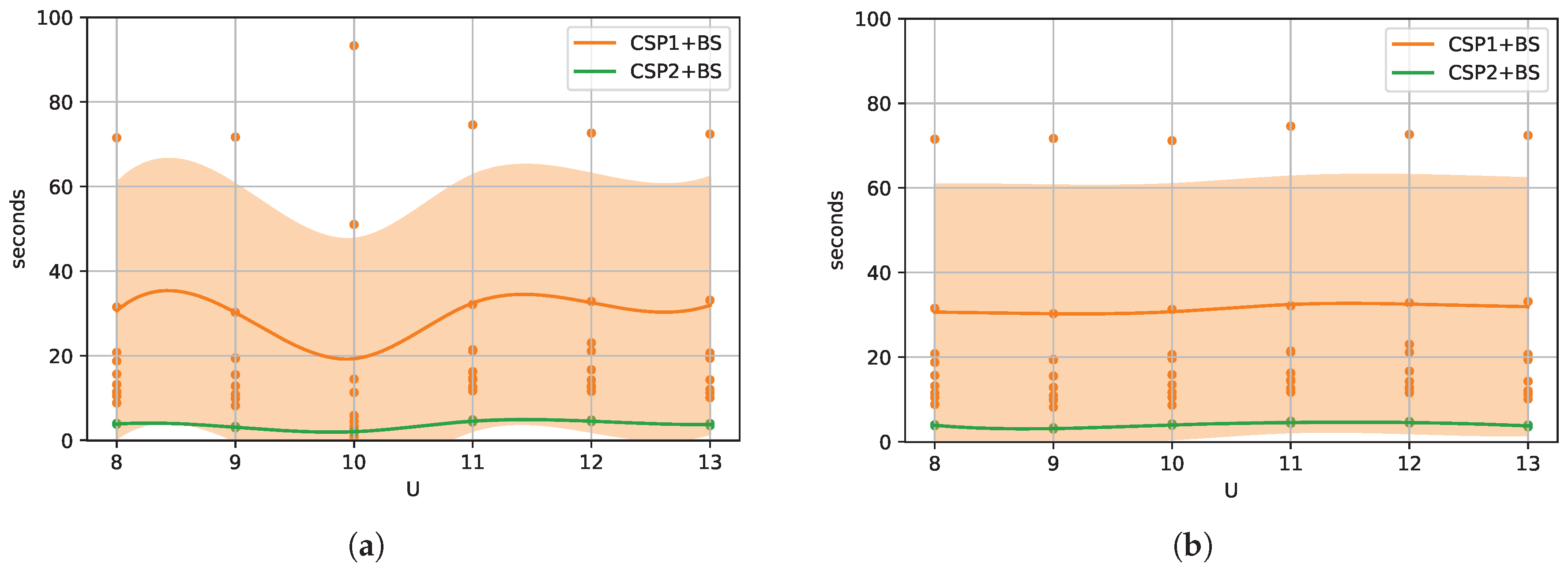
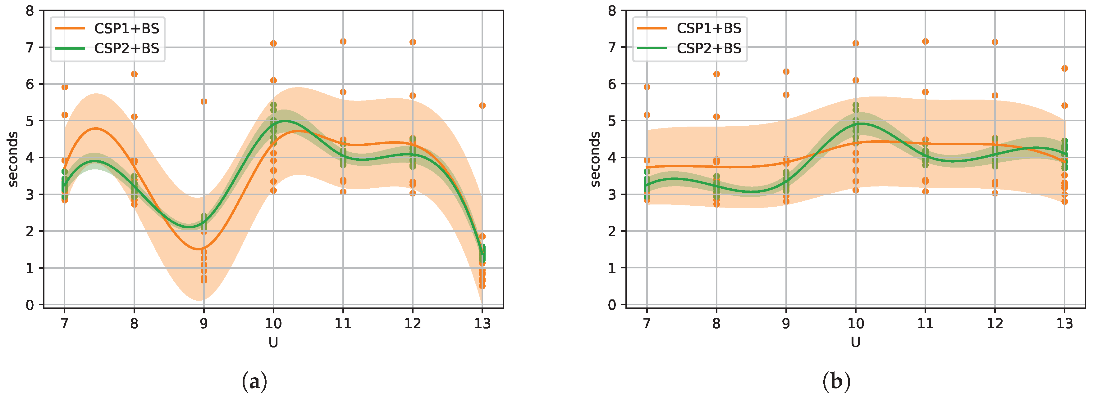
By the previous set of experiments, it seems likely that CSP1 + BS would be very inefficient over graphs with a burning number of seven or more. Therefore, we executed CSP1 + BS over graphs with an upper bound on the burning number of six or less. Furthermore, since CSP1 + BS has fewer memory requirements than CSP2 + BS, we could execute the former over graphs of order up to 5908. Regarding CSP2 + BS, we executed it over graphs with an upper bound on the burning number of at least seven and order at most 1458 because Gurobi’s branch-and-bound algorithm exhausted all available memory when executed over bigger graphs. This way, the results reported in Table 3 confirm the optimality of most previously known solutions. Furthermore, the optimal solution of some graphs is reported for the first time (ca-netscience, web-polblogs, DD68, DD199, DD497, lattice2D, and tech-routers-rf). The TVshow graph could not be solved within ∼48 h using CSP1 + BS; this goes along with the observation that CSP1 + BS does not seem adequate for solving graphs with a relatively large burning number. From Table 3, we also observe that synthetic graphs with a well-defined structure seem more challenging to solve. For instance, lattice3D required 150,000 s (∼42 h) to be solved using CSP2 + BS. In order to find optimal solutions for challenging graphs, we executed CSP1 + BS and CSP2 + BS over some grid graphs (See Table 4). As before, we executed CSP1 + BS and CSP2 + BS over graphs with a known upper bound of at most six and at least seven, respectively. From Table 4, we can observe that the implemented formulations found twelve optimal solutions that the state-of-the-art heuristics could not find.

6. Discussion

This paper introduces three novel mathematical formulations for the GBP: an ILP and two CSPs (CSP1 and CSP2). Since CSP1 and CSP2 require the burning number in advance, they are integrated into a binary search procedure (CSP1 + BS and CSP2 + BS); this way, the issue of not knowing the burning number in advance is lessened. All these formulations can be solved over arbitrary graphs thanks to off-the-shelf optimization software.
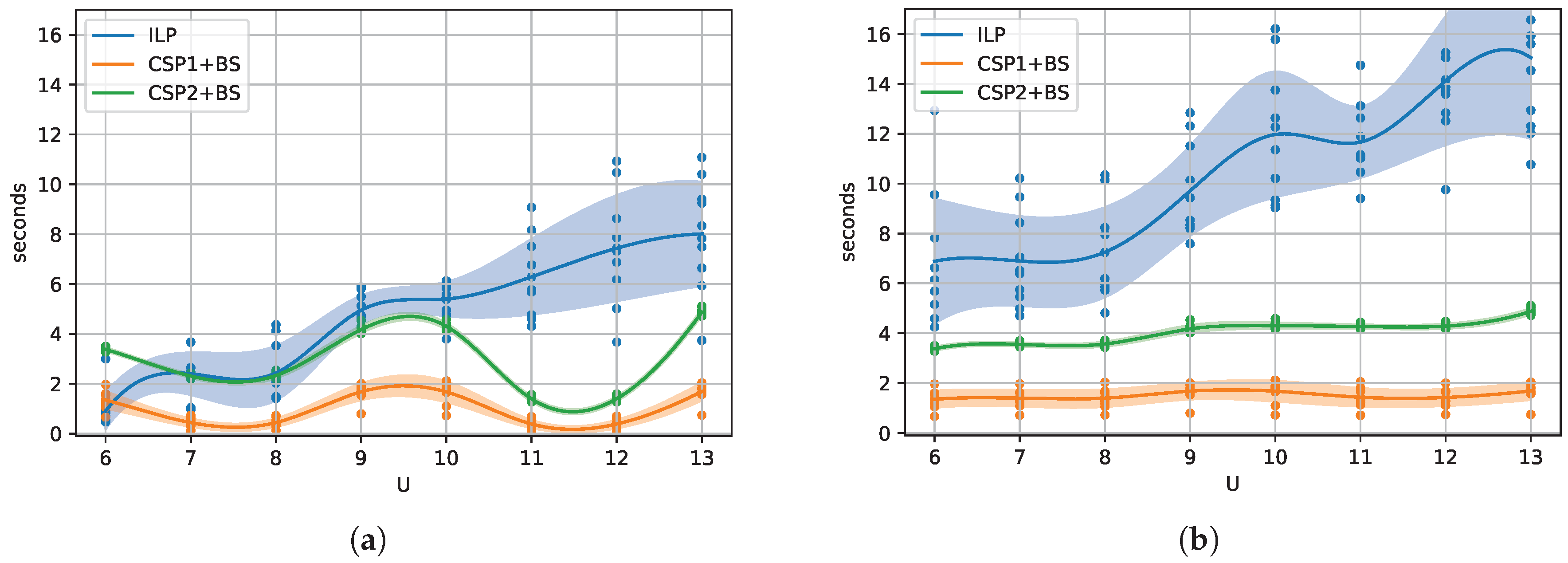
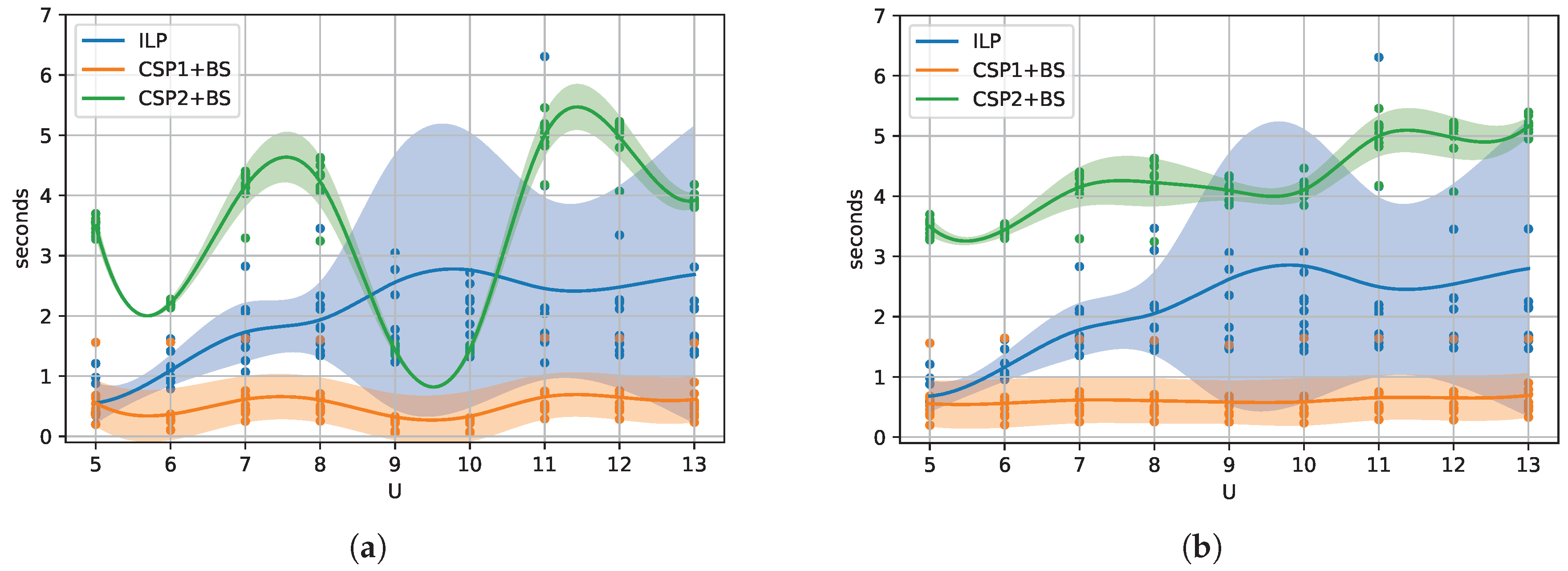
Section 4 shows a series of experiments that validate the correct implementation of the proposed formulations. This same section presents an empirical performance comparison among them using random graphs. From these experiments, we observe that CSP2 + BS tends to be better suited for graphs with a relatively large burning number (we empirically estimated this value as seven or more.) From these same experiments, we observe that CSP1 + BS seems to be a better choice for solving graphs with a relatively small burning number (we empirically estimated this value as six or less.) Of course, these observations cannot be generalized. Thus, rigorous statistical analysis should be performed in the future.
In Section 5, we used CSP1 + BS and CSP2 + BS to compute the optimal solution for some benchmark connected graphs of order at most 5908 (it is worth mentioning that, in all experiments, the BNC holds.) From these, we found seven previously unknown optimal solutions. We could not apply CSP2 + BS over graphs of order greater than 1458 because the memory requirements grew beyond our hardware’s capacity. Regarding CSP1 + BS, it solved graphs with a relatively small burning number and order at most 5908. The obtained set of optimal solutions can be helpful as a benchmark dataset for comparing non-exact algorithms for the GBP, i.e., approximation algorithms, heuristics, and metaheuristics.
Finally, as part of the reviewing process, a reviewer pointed to the possibility of reducing the number of variables and constraints from CSP2 by removing variables x i and y i , j . However, we believe such variables cannot be removed because they let us guarantee that the solution has length B and that all vertices are burned. Nevertheless, we agree that mathematical formulations with fewer variables and constraints might exist. Thus, we will seek alternative mathematical formulations of the problem for future work.

Author Contributions

Conceptualization, J.G.-D., L.M.X.R.-H., J.C.P.-S. and S.E.P.-H.; methodology, J.G.-D., L.M.X.R.-H., J.C.P.-S. and S.E.P.-H.; software, J.G.-D.; validation, J.G.-D., L.M.X.R.-H., J.C.P.-S. and S.E.P.-H.; formal analysis, J.G.-D., L.M.X.R.-H., J.C.P.-S. and S.E.P.-H.; investigation, J.G.-D., L.M.X.R.-H., J.C.P.-S. and S.E.P.-H.; data curation, J.G.-D.; writing—original draft preparation, J.G.-D.; writing—review and editing, J.G.-D., L.M.X.R.-H., J.C.P.-S. and S.E.P.-H. All authors have read and agreed to the published version of the manuscript.

Funding

This research received no external funding.

Institutional Review Board Statement

Not applicable.

Informed Consent Statement

Not applicable.

Data Availability Statement

The data presented in this paper are openly available in https://github.com/jesgadiaz/GBP (acccessed on 31 July 2022).

Acknowledgments

We thankfully acknowledge Gurobi for providing a free-of-charge academic license for Gurobi version 9.5.1. We are grateful to anonymous reviewers whose questions, comments, and suggestions helped improve an earlier version of this paper. We also acknowledge Consejo Nacional de Ciencia y Tecnología (CONACYT) and Instituto Nacional de Astrofísica, Óptica y Electrónica (INAOE) for providing the necessary resources for the development of this research. The authors thankfully acknowledge the computer resources, technical expertise and support provided by the Laboratorio Nacional de Supercómputo del Sureste de México, CONACYT member of the network of national laboratories.

Conflicts of Interest

The authors declare no conflict of interest.

Abbreviations

The following abbreviations are used in this manuscript:
BBGHBackbone based greedy heuristic
BFFBurning farthest-first
BNCBurning number conjecture
BSBinary search
CBRHComponent based recursive heuristic
CSPConstraint satisfaction problem
FPFirefighter problem
GBPGraph burning problem
ICCHImproved cutting corners heuristic
ILPInteger linear program
VKCPVertex k-center problem

References

  1. Bonato, A.; Janssen, J.; Roshanbin, E. Burning a graph as a model of social contagion. In International Workshop on Algorithms and Models for the Web-Graph; Springer: Berlin/Heidelberg, Germany, 2014; pp. 13–22. [Google Scholar]
  2. Bessy, S.; Bonato, A.; Janssen, J.; Rautenbach, D.; Roshanbin, E. Burning a graph is hard. Discret. Appl. Math. 2017, 232, 73–87. [Google Scholar] [CrossRef]
  3. Diestel, R. Graph Theory; Springer Graduate Texts in Mathematics; Springer: Berlin/Heidelberg, Germany, 2017. [Google Scholar]
  4. Šimon, M.; Huraj, L.; Luptáková, I.D.; Pospíchal, J. Heuristics for spreading alarm throughout a network. Appl. Sci. 2019, 9, 3269. [Google Scholar] [CrossRef] [Green Version]
  5. Gautam, R.H.; Kare, A.S.; Surampudi, D.B. Faster heuristics for graph burning. Appl. Intell. 2021, 52, 1351–1361. [Google Scholar] [CrossRef] [PubMed]
  6. Gupta, A.T.; Lokhande, S.A.; Mondal, K. Burning grids and intervals. In Proceedings of the Algorithms and Discrete Applied Mathematics, Rupnagar, India, 11–13 February 2021; pp. 66–79. [Google Scholar]
  7. Bonato, A.; Kamali, S. Approximation algorithms for graph burning. In Proceedings of the International Conference on Theory and Applications of Models of Computation, Kitakyushu, Japan, 13–16 April 2019; pp. 74–92. [Google Scholar]
  8. García-Díaz, J.; Pérez-Sansalvador, J.C.; Rodríguez-Henríquez, L.M.X.; Cornejo-Acosta, J.A. Burning Graphs Through Farthest-First Traversal. IEEE Access 2022, 10, 30395–30404. [Google Scholar] [CrossRef]
  9. Vazirani, V.V. Approximation Algorithms; Springer Science & Business Media: Berlin/Heidelberg, Germany, 2013. [Google Scholar]
  10. Bonato, A.; English, S.; Kay, B.; Moghbel, D. Improved bounds for burning fence graphs. Graphs Comb. 2021, 37, 2761–2773. [Google Scholar] [CrossRef]
  11. Liu, H.; Zhang, R.; Hu, X. Burning number of theta graphs. Appl. Math. Comput. 2019, 361, 246–257. [Google Scholar] [CrossRef]
  12. Bonato, A.; Lidbetter, T. Bounds on the burning numbers of spiders and path-forests. Theor. Comput. Sci. 2019, 794, 12–19. [Google Scholar] [CrossRef] [Green Version]
  13. Liu, H.; Hu, X.; Hu, X. Burning number of caterpillars. Discret. Appl. Math. 2020, 284, 332–340. [Google Scholar]
  14. Mitsche, D.; Prałat, P.; Roshanbin, E. Burning number of graph products. Theor. Comput. Sci. 2018, 746, 124–135. [Google Scholar] [CrossRef] [Green Version]
  15. Sim, K.A.; Tan, T.S.; Wong, K.B. On the burning number of generalized petersen graphs. Bull. Malaysian Math. Sci. 2018, 41, 1657–1670. [Google Scholar] [CrossRef]
  16. Bastide, P.; Bonamy, M.; Bonato, A.; Charbit, P.; Kamali, S.; Pierron, T.; Rabie, M. Improved Pyrotechnics: Closer to the Burning Number Conjecture. Preprint. 2022. Available online: https://arxiv.org/abs/2110.10530 (accessed on 31 July 2022).
  17. Gonzalez, T.F. Clustering to minimize the maximum intercluster distance. Theor. Comput. Sci. 1985, 38, 293–306. [Google Scholar] [CrossRef] [Green Version]
  18. Hochbaum, D.S.; Shmoys, D.B. A best possible heuristic for the k-center problem. Math. Oper. Res. 1985, 10, 180–184. [Google Scholar] [CrossRef] [Green Version]
  19. Garcia-Diaz, J.; Menchaca-Mendez, R.; Menchaca-Mendez, R.; Hernández, S.P.; Pérez-Sansalvador, J.C.; Lakouari, N. Approximation Algorithms for the Vertex K-Center Problem: Survey and Experimental Evaluation. IEEE Access 2019, 7, 109228–109245. [Google Scholar] [CrossRef]
  20. Cornejo Acosta, J.A.; García Díaz, J.; Menchaca-Méndez, R.; Menchaca-Méndez, R. Solving the Capacitated Vertex K-Center Problem through the Minimum Capacitated Dominating Set Problem. Mathematics 2020, 8, 1551. [Google Scholar] [CrossRef]
  21. Grandoni, F. A note on the complexity of minimum dominating set. J. Discret. Algorithms 2006, 4, 209–214. [Google Scholar] [CrossRef] [Green Version]
  22. Hernández-Gómez, J.C.; Reyna-Hérnandez, G.; Romero-Valencia, J.; Rosario Cayetano, O. Transitivity on Minimum Dominating Sets of Paths and Cycles. Symmetry 2020, 12, 2053. [Google Scholar] [CrossRef]
  23. Hartnell, B. Firefighter! An application of domination. Presentation. In Proceedings of the 25th Manitoba Conference on Combinatorial Mathematics and Computing, Winnipeg, MB, Canada, 29 September–1 October 1995. [Google Scholar]
  24. Develin, M.; Hartke, S.G. Fire containment in grids of dimension three and higher. Discrete Appl. Math. 2007, 155, 2257–2268. [Google Scholar] [CrossRef] [Green Version]
  25. García-Martínez, C.; Blum, C.; Rodriguez, F.J.; Lozano, M. The firefighter problem: Empirical results on random graphs. Comput. Oper. Res. 2015, 60, 55–66. [Google Scholar] [CrossRef]
  26. Kozen, D.C. Depth-First and Breadth-First Search. In The Design and Analysis of Algorithms; Texts and Monographs in Computer Science; Springer: New York, NY, USA, 1992. [Google Scholar] [CrossRef]
  27. Gurobi Optimization. Gurobi Optimizer Reference Manual. 2022. Available online: http://www.gurobi.com/documentation/9.5/refman (accessed on 31 July 2022).
  28. Erdos, P.; Rényi, A. On the evolution of random graphs. Publ. Math. Inst. Hung. Acad. Sci. 1960, 5, 17–60. [Google Scholar]
  29. Rossi, R.A.; Ahmed, N.K. The Network Data Repository with Interactive Graph Analytics and Visualization. AAAI. 2015. Available online: http://networkrepository.com (accessed on 31 July 2022).
  30. Leskovec, J.; Krevl, A. Snap Datasets: Stanford Large Network Dataset Collection. 2014. Available online: http://snap.stanford.edu/data (accessed on 31 July 2022).
Figure 1. An optimal burning sequence for a nine vertices path is ( v 3 , v 7 , v 9 ) . The burning process of this sequence is depicted by each i { 1 , 2 , 3 } with its corresponding steps a and b. Notice that vertex v 3 burns all vertices in N 2 [ v 3 ] , vertex v 7 burns all vertices in N 1 [ v 7 ] , and vertex v 9 burns all vertices in N 0 [ v 9 ] .
Mathematics 10 02777 g001
Figure 2. Optimal burning sequence ( s 1 , s 2 , , s b ( G ) ) of (a) a two-dimensional lattice, (b) a three-dimensional lattice, (c) the ca-netscience graph, (d) the karate-club graph, (e) the DD199 graph, and (f) the web-polblogs graph.
Mathematics 10 02777 g002
Figure 3. (a) Time to the optimal solution and (b) to proven optimality reported by Gurobi for the CSP1 + BS and CSP2 + BS over 10 random graphs of order 100, p = 0.02 , and b ( G ) = 8 . The bounds are L = 1 and U [ b ( G ) , ( 4 · 100 / 3 ) 1 / 2 + 1 ] .
Mathematics 10 02777 g003
Figure 4. (a) Time to the optimal solution and (b) to proven optimality reported by Gurobi for the CSP1 + BS and CSP2 + BS over 10 random graphs of order 100, p = 0.023 , and b ( G ) = 7 . The bounds are L = 1 and U [ b ( G ) , ( 4 · 100 / 3 ) 1 / 2 + 1 ] .
Mathematics 10 02777 g004
Figure 5. (a) Time to the optimal solution and (b) to proven optimality reported by Gurobi for the ILP, CSP1 + BS, and CSP2 + BS over 10 random graphs of order 100, p = 0.03 , and b ( G ) = 6 . The bounds are L = 1 and U [ b ( G ) , ( 4 · 100 / 3 ) 1 / 2 + 1 ] .
Mathematics 10 02777 g005
Figure 6. (a) Time to the optimal solution and (b) to proven optimality reported by Gurobi for the ILP, CSP1 + BS, and CSP2 + BS over 10 random graphs of order 100, p = 0.04 , and b ( G ) = 5 . The bounds are L = 1 and U [ b ( G ) , ( 4 · 100 / 3 ) 1 / 2 + 1 ] .
Mathematics 10 02777 g006
Table 1. Running time of the implemented mathematical formulations over a set of paths.
PathsBoundsILPCSP1 + BSCSP2 + BS
| V | | E | ρ b ( G ) L U t o t p t o t p t o t p
16150.1254260.0590.0680.0150.0160.0160.060
25240.0805370.2310.2390.0160.0780.0230.173
36350.0566481.0863.90.1840.6370.0780.410
49480.04175986.4242.21.55.20.1480.769
64630.031861023.9>20002.3105.90.2501.3
81800.0259711>2000>200021.0202.40.4292.2
100990.02010812>2000>2000>2000>20001.03.8
1211200.01711913>2000>2000>2000>20002.26.4
1441430.014121014>2000>2000>2000>20001.88.1
1691680.012131115>2000>2000>2000>20003.012.3
1961950.010141216>2000>2000>2000>20005.619.1
2252240.009151317>2000>2000>2000>200016.836.9
2562550.008161418>2000>2000>2000>2000142.9170.7
2892880.007171519>2000>2000>2000>200063.8100.7
3243230.006181620>2000>2000>2000>2000126.1177.7
3613600.006191721>2000>2000>2000>2000347.4417.7
Table 2. Running time of the implemented mathematical formulations over a set of connected tight examples for the BFF algorithm.
BFF’s Connected Tight ExamplesBoundsILPCSP1 + BSCSP2 + BS
| V | | E | ρ b ( G ) L U t o t p t o t p t o t p
650.3332140.0090.0120.0010.0040.0020.014
19180.1053150.0160.0160.0010.0110.0120.080
40390.0504260.1100.1100.0010.0420.0560.354
69680.0295370.6620.6620.1100.1880.2211.2
1061050.1896486.06.00.7010.8740.6293.1
1511500.01375931.031.04.95.41.36.8
2042030.0108610449.8449.84.56.72.913.5
2652640.0089711>2000>2000140014005.824.9
3343330.00610812>2000>20001900190011.544.5
4114100.00511913>2000>2000>2000>200021.175.3
4964950.004121014>2000>2000>2000>200040.1139.1
5895880.003131115>2000>2000>2000>200068.2232.4
6906890.003141216>2000>2000>2000>2000102.1336.2
7997980.003151317>2000>2000>2000>2000172.8528.8
9169150.002161418>2000>2000>2000>2000256.3799.7
104110400.002171519>2000>2000>2000>2000349.11100
Table 3. Optimal solutions found by CSP1 + BS and CSP2 + BS over some benchmark graphs. The feasible solutions found by some state-of-the-art algorithms are reported too. Optimal solutions reported for the first time are underlined.
GraphsBounds t p BFFHeuristics
Name | V | | E | ρ b ( G ) L U CSP1 + BSCSP2 + BSWorstBestICCHBBGHCBRH
karate-club34780.1393330.015-53334
chesapeake391700.2293230.023-43333
dolphins621590.0844340.103-74455
rt-retweet961170.0265450.125-95555
polbooks1054410.0814340.157-64445
adjnoun1124250.0684340.160-64444
ia-infect-hyper11321960.3473230.350-43333
C125-912569630.8983230.924-33333
ia-enron-only1436230.0614340.350-75544
c-fat200-120015340.077737-13.977777
c-fat200-220032350.16353521.7-55555
c-fat200-520084730.4263231.1-33333
sphere325810260.031747-27.498777
DD2442918220.019757-23.5129777
ca-netscience3799140.013657-46.1118777
infect-dublin41027650.03354528.2-85555
c-fat500-150044590.036959-112.511101099
c-fat500-250091390.073747-120.387777
c-fat500-550023,1910.186535297.3-55555
bio-diseasome51611880.009757-122.5137778
web-polblogs64322800.0115466.7-106666
rt-twitter-copen76110290.004757-805.7137777
DD6877520930.0079610-491.81611101010
ia-crime-moreno82914750.004747-1800107777
DD19984119020.00512814-672.52116141414
soc-wiki-Vote88929140.00765621.6-116666
DD49790324530.00610712-836.71814111112
socfb-Reed9896218,8120.0414346.7-74444
lattice3D100027000.00510610-150,0001411101011
bal_bin_tree_9102310220.00210710-381.91810111010
delaunay_n10102430560.006959-1100131010910
stufe103618680.00312712-13001814131213
lattice2D108921120.00413814-28002016151414
bal_ter_tree_6109310920.002757-260.1137977
email-univ113354510.009545208.7-95666
econ-mahindas125875130.010545128.1-85555
ia-fb-messages126664510.00854555.2-95555
bio-yeast145819480.002979-12,000179999
tech-routers-rf211366320.003657252.1-127777
chameleon227731,4210.0126568.2-116666
TVshow389217,2620.002?710--1810101010
ego-facebook403988,2340.0114341800-75444
squirrel5201198,4930.015646170,000-106666
politician590841,7290.00275721,000-137777
Table 4. Optimal solutions found by CSP1 + BS and CSP2 + BS over some square grid graphs. The feasible solutions found by some state-of-the-art algorithms are reported too. Optimal solutions reported for the first time are underlined.
n × n GridsBounds t p BFFHeuristics
n | V | | E | ρ b ( G ) L U CSP1 + BSCSP2 + BSWorstBestICCHBBGHCBRH
39120.3333230.001-43333
416240.2004240.031-44444
525400.1334340.047-54445
636600.0955350.235-65555
749840.0715350.539-75556
8641120.0566369.1-76666
9811440.04464611.3-86666
101001800.036647-2.597777
111212200.030747-5.2107777
121442640.026747-7.2108878
131693120.022758-7.5118888
141963640.019858-14.5119988
152254200.017859-15.4129999
162564800.015859-17.21210999
172895440.013959-35.7121010910
183246120.012959-46.2131110910
193616840.0119510-65.51311101010
204007600.01010610-108.01411111011
214418400.00910610-119.11412111011
224849240.00810611-200.11512111111
2352910120.00711611-234.31512121111
2457611040.00711611-332.91613121112
2562512000.00611612-432.81613121212
2667613000.00611712-807.41713131212
2772914040.00512712-819.41714131212
2878415120.00512712-746.31814131212
2984116240.00512713-18001814131313
3090017400.00412713-75001915141313
3196118600.00413713-16001915141313
32102419840.00413813-15002015141313
33108921120.00413814-30002016151414
34115622440.00313814-66002016151414
35122523800.00314814-68002116151415
Publisher’s Note: MDPI stays neutral with regard to jurisdictional claims in published maps and institutional affiliations.

