Constrained Optimal Control for Nonlinear Multi-Input Safety-Critical Systems with Time-Varying Safety Constraints

Abstract

In this paper, we investigate the constrained optimal control problem of nonlinear multi-input safety-critical systems with uncertain disturbances and time-varying safety constraints. By utilizing a barrier function transformation, together with a new disturbance-related term and a smooth safety boundary function, a nominal system-dependent multi-input barrier transformation architecture is developed to deal with the time-varying safety constraints and uncertain disturbances. Based on the obtained transformation system, the coupled Hamilton–Jacobi–Bellman (HJB) function is established to obtain the constrained Nash equilibrium solution. In addition, due to the fact that it is difficult to solve the HJB function directly, the single critic neural network (NN) is constructed to approximate the optimal performance index function of different control inputs, respectively. It is proved theoretically that, under the influence of uncertain disturbances and time-varying safety constraints, the system states and neural network parameters can be uniformly ultimately bounded (UUB) by the proposed neural network approximation method. Finally, the effectiveness of the proposed method is verified by two nonlinear simulation examples.

1. Introduction

To solve the optimal control problem of any safety-critical systems (e.g., autonomous vehicles, intelligent robots, etc.), safety should be the basic requirement. Failure to ensure the safety of such systems may result in serious consequences, such as casualties, environmental pollution, and equipment damage. The safety control design refers to the control strategy which satisfies the safety specification stipulated by the physical or environmental constraints of the system. The barrier function (BF) method [1,2] has been proved to be an effective method to realize the system safety constraints or state constraints, and have attracted a wide amount of attention in recent years. For the optimal control problem in the modern control domain, it usually relies on solving the complex Hamilton–Jacobi–Bellman (HJB) equation [3,4,5]. However, there is no effective mathematical method to solve the HJB equation due to its own properties. When designing the controllers that are both safe and optimal, the proper combination of safety and performance goal is an issue worth studying.

It has been proved that the dynamic programming (DP) method is a feasible and effective method to solve the HJB equation and derive the optimal solution. However, as the dimension of the variables increases, the dynamic programming method suffers from the “dimension curse”. Adaptive dynamic programming (ADP) [6,7,8,9,10] uses the function approximation, such as neural network (NN) approximation methods, to approximate the cost function in the HJB equation, which has been proved to be a valid method to solve the dimension curse of dynamic programming method. It is an emerging method combining the development of artificial intelligence and control field, and has become a hotspot of international optimization research in recent years [11,12,13,14,15]. In [11,12,13], the authors studied the optimal control problem with disturbance by using the reinforcement learning (RL) method. Aiming at the random differential equations systems with coexisting parametric uncertainties and severe nonlinearities, Zhang et al. [14] studied the problem of event-triggered adaptive tracking control. Vamvoudakis et al. [15] proposed an online continuous time learning algorithm based on policy iteration to learn the optimal control solutions of known nonlinear systems. In [16,17,18], the robust control problem was transformed into the optimal control problem of the nominal system by selecting an appropriate utility function. On the other hand, game theory [19,20,21,22,23,24] has become a powerful tool to optimize the coordination and cooperation of multiple controllers, and has been proved in many practical control problems. In fact, many systems in the real world have the idea of the non-zero-sum (NZS) game, where each controller of the system tries to minimize its cost function. Many researchers translate the non-zero-sum game problem [25,26] into the problem of solving the coupled HJB equation, but it is still a great difficulty to solve the coupled HJB equation [27,28,29]. The development of adaptive dynamic programming and game theory has prompted many scholars to conduct relevant research. For robust trajectory tracking multiple input control of uncertain nonlinear systems, Qin et al. [28] proposed a new adaptive online learning method to learn the Nash equilibrium solution. Song et al. [29] developed a non-strategic integral reinforcement learning (IRL) method to effectively solve the NZS game control problem with unknown system dynamics. Ming et al. [30] proposed a single-network adaptive control method to obtain the optimal solution of NZS differential game for autonomous nonlinear systems. All of the above methods can effectively solve the NZS game optimal control problem. However, few studies have been done on the NZS game with disturbance and time-varying safety constraints. This prompted the author to study this problem.

For the safety constraints, the existing methods based on barrier function and adaptive dynamic programming have received a lot of attention in recent years. Marvi et al. [31] proposed a barrier certified method to learn the safety optimal controller and ensure the operation of the safety-critical system within its safety zone while providing the optimal performance. By introducing the barrier function into utility function, Xu et al. [32] augmented the penalty mechanism to the utility function, and solved the state constraints problem that was difficult to be dealt with by the traditional ADP method. Liu et al. [33] proposed an adaptive control method to obtain the safety solution of nonlinear stochastic systems. In addition, the barrier function transformation method has proved that it is possible to transform the safety-critical system with safety constraints into a general system without constraints in different scenarios, such as zero-sum game [34], non-zero-sum game [35], tracking control [36], and event-triggered control [37]. However, without exception, the above results must satisfy the implicit assumption that the safety constraints are constant. In fact, the constant constraint is only a special case of time-varying constraints. In practical applications, the time-varying constraints also have a wide range of application scenarios, such as UAV or manipulator working in some more complex environments.

For the constrained optimal control problem with time-varying safety constraints and uncertain disturbances, the constrained Nash equilibrium solutions are obtained by introducing a novel barrier function transformation and constructing coupled HJB equations. The novelty of this paper is reflected in the following points:

(1). A novel barrier function transformation method is proposed by introducing a smooth safety boundary function and a barrier function with a single variable. Compared to previous works [34,35], the proposed method no longer strictly requires the time-invariance of safety constraints and can deal with both time-invariance and time-varying safety constraints.

(2). In order to obtain the constrained optimal Nash equilibrium solution of the multi-input barrier transformation system with uncertain disturbances, the reasonable performance index function and coupled HJB function are designed for the nominal system by introducing a disturbance-related term. It is proved that the obtained constrained Nash equilibrium solution can make the safety-critical system asymptotically stable under the uncertain disturbances and time-varying safety constraints.

(3). The single critical neural network is used to approximate the performance index function online to obtain the constrained control input. It is proved theoretically that the proposed barrier function transformation and neural network approximation method can make the system state and NN parameters uniformly ultimately bounded (UUB) under the condition of satisfying the time-varying safety constraints. In addition, two simulation examples also verify the feasibility and effectiveness of the proposed method.

The remainder of this article is organized as follows: Problem formulation and barrier transformation are given in Section 2. Section 3 employs the coupled Hamilton–Jacobi–Bellman equation to obtain the approximate optimal solution online. Section 4 shows the efficiency of the proposed method by giving two simulation examples. Finally, conclusions are given in Section 5.

2. Problem Formulation and Barrier Transformation

Consider the following nonlinear multi-input safety-critical system:

$$\begin{array}{c}\hfill \dot{x}=f(x(t))+g_1(x(t))u_1(t)+g_2(x(t))u_2(t)+k(x(t))d(\phi (x(t))),\end{array}$$

(1)

where $x\in C\subset R^n$ is the system state, $u_1\in U_1\subset R^{m_1}$, $u_2\in U_2\subset R^{m_2}$ are the control inputs, $d(\phi (x(t)))\in R^m$ is the uncertain disturbance, $f(x)\in R^n$, $g_1(x)\in R^{n\times m_1}$, $g_2(x)\in R^{n\times m_2}$ and $k(x)\in R^{n\times m}$. C indicates the set of acceptable system state, and $U_1,U_2$ indicates the set of acceptable system inputs. It is supposed that $f(x),g_1(x),g_2(x)$ is Lipschitz continuous, and $f(0)=0$. It is also assumed that the system (1) is stabilizable. The uncertain disturbance term d satisfies $d^{T}d<{\delta }^T\delta$, where $\delta$ is a given function, $\delta (0)=0$ and $\phi (·)$ satisfy that $\phi (0)=0$ is a fixed function denoting the uncertainty.

Given the initial system state $x_0$, the purpose of this article is to find the constrained control inputs $u_1,u_2$ to make the system state x converge to the ideal value under the impact of the uncertain disturbances and time-varying safety constraints.

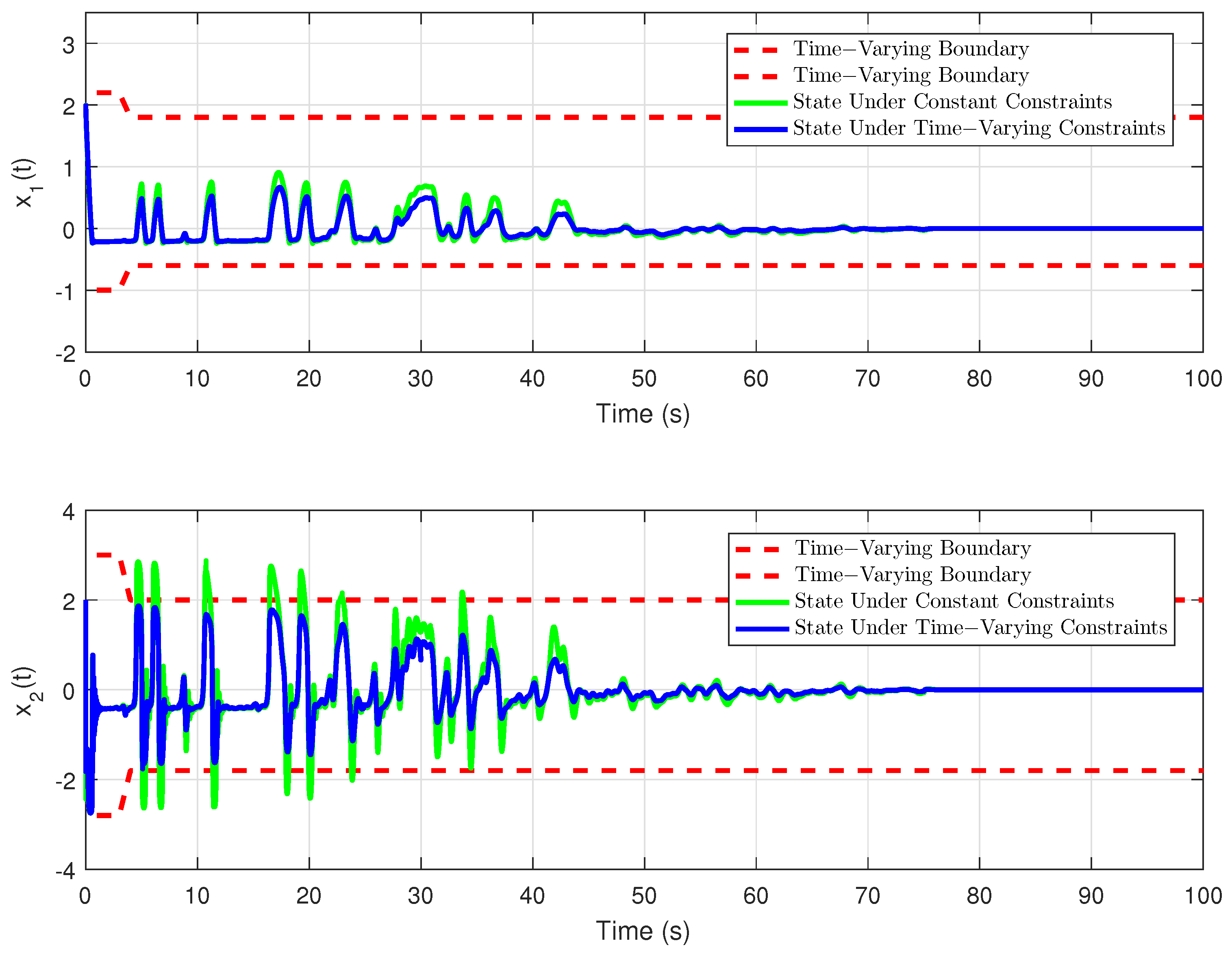
Remark 1.

In some papers, for example [31,35], the system state is constrained by the constant, that is, $x\in ({\zeta }_a,{\zeta }_A)$, where $({\zeta }_a,{\zeta }_A)$ represent the upper and lower bounds of system state. We consider a more complex and interesting case where the system safety constraints are time-varying and can be mathematically expressed as $x\in ({\zeta }_a(t),{\zeta }_A(t))$, where $({\zeta }_a(t),{\zeta }_A(t))$ represent the bounded smooth time-varying functions.

In order to satisfy the time-varying safety constraints, we define the following barrier function with a single independent variable $\tau$,

$$\begin{array}{ccc}& & b(z(\tau );{\xi }_a(\tau ),{\xi }_A(\tau ))=log\frac{{\xi }_A(\tau )({\xi }_a(\tau )-z(\tau ))}{{\xi }_a(\tau )({\xi }_A(\tau )-z(\tau ))},\hfill \end{array}$$

(2)

$$\begin{array}{ccc}& & b^{-1}(y(\tau );{\xi }_a(\tau ),{\xi }_A(\tau ))={\xi }_a(\tau ){\xi }_A(\tau )\frac{e^{\frac{y(\tau )}{2}}-e^{-\frac{y(\tau )}{2}}}{{\xi }_a(\tau )e^{\frac{y(\tau )}{2}}-{\xi }_A(\tau )e^{-\frac{y(\tau )}{2}}},\hfill \end{array}$$

(3)

where ${\xi }_a(·):R\to R$, ${\xi }_A(·):R\to R$, $z(·):R\to R$, $y(·):R\to R$. The defined barrier function should satisfy the following assumption.

Assumption 1.

The proposed barrier function $b(·)$ has the following characteristics:

(1) ${\xi }_a(\tau )$, ${\xi }_A(\tau )$ are two smooth functions and satisfy ${\xi }_a(\tau )<0<{\xi }_A(\tau )$ for any $\tau >0$;

(2) For any $\tau >0$, the barrier function takes finite value when $z(\tau )\in ({\xi }_a(\tau ),{\xi }_A(\tau ))$ is satisfied;

(3) For any $\tau >0$, as the function $z(\tau )$ tends to the prescribed region $({\xi }_a(\tau ),{\xi }_A(\tau ))$, $b(·)$ approaches infinity, i.e., $\underset{z(\tau )\to {\xi }_a{(\tau )}^{+}}{lim}b(z(\tau );{\xi }_a(\tau ),{\xi }_A(\tau ))=-\infty$, $\underset{z(\tau )\to {\xi }_A{(\tau )}^{-}}{lim}b(z(\tau );{\xi }_a(\tau ),{\xi }_A(\tau ))$

$=+\infty$;

(4) For any $\tau >0$, the barrier function $b(·)$ also converges when the function $z(\tau )$ converges.

It is worth noting that the constraints given by $({\zeta }_a(t),{\zeta }_A(t))$ can be many common trajectories, including sinusoidal waveforms, damping sinusoids, ramp, and so on. In our study, we will discuss a more useful form. We design the constraints $({\zeta }_a(t),{\zeta }_A(t))$ as the following smooth transformation functions, and satisfy the following conditions:

$$\begin{array}{c}\hfill {\zeta }_a(t)=\left[\begin{array}{c}{\zeta }_{a1}(t)\\ ⋮\\ {\zeta }_{an}(t)\end{array}\right],{\zeta }_{ai}(t)=\left\{\begin{array}{cc}& l_1,t<t_1\hfill \\ & l_1-{\vartheta }_1-{\vartheta }_{1}cos(\pi \frac{t_2-t}{t_2-t_1}),t_1\le t\le t_2\hfill \\ & l_2,t>t_2\hfill \end{array}\right.\end{array}$$

(4)

$$\begin{array}{c}\hfill {\zeta }_A(t)=\left[\begin{array}{c}{\zeta }_{A1}(t)\\ ⋮\\ {\zeta }_{An}(t)\end{array}\right],{\zeta }_{Ai}(t)=\left\{\begin{array}{cc}& l_3,t<t_3\hfill \\ & l_3-{\vartheta }_2-{\vartheta }_{2}cos(\pi \frac{t_4-t}{t_4-t_3}),t_3\le t\le t_4\hfill \\ & l_4,t>t_4\hfill \end{array}\right.\end{array}$$

(5)

where $i=1,\cdots ,n$, $l_1<0$, $l_2<0$, $l_3>0$, $l_4>0$, and $l_1-2{\vartheta }_1=l_2$, $l_3-2{\vartheta }_2=l_4$. We can find many similar practical applications where the similar constraints are imposed (e.g., vehicle entering a narrow road from a wide road, drone entering a tunnel, robotic arm working in a narrow space, etc.).

Remark 2.

A reasonable choice of parameters can be such that $l_1=l_2$, $l_3=l_4$ when designing a smooth transformation function. In other words, the proposed method can also impose time-invariant safety constraints on the system state when some parameters are selected properly. In addition, according to the defined smooth transformation function, it can be extended to scenarios with more complex safety requirements, such as more frequent transformation of constraints and different types of constraints.

Considering the system (1) with the uncertain disturbances and time-varying safety constraints, we use the proposed barrier function and smooth transformation function to convert the multi-input safety-critical system x with the uncertain disturbances and time-varying safety constraints into the transformation system with uncertain disturbances only. We define

$$\begin{array}{ccc}& & s_i=b(x_i(t);{\zeta }_{ai}(t),{\zeta }_{Ai}(t)),\hfill \end{array}$$

(6)

$$\begin{array}{ccc}& & x_i=b^{-1}(s_i(t);{\zeta }_{ai}(t),{\zeta }_{Ai}(t)).\hfill \end{array}$$

(7)

According to the chain rule and Equations (6) and (7), the transformed system dynamics $\dot{s}$ can be defined as

$$\begin{array}{ccc}\hfill {\dot{s}}_i& & =\frac{{\dot{x}}_i}{\frac{d{b}^{-1}(s_i(t);{\zeta }_{ai}(t),{\zeta }_{Ai}(t))}{d{s}_i}},\hfill \\ & & =\frac{f_i(x(t))+g_{1i}(x(t))u_1(t)+g_{2i}(x(t))u_2(t)+k_i(x(t))d(\phi (x(t)))}{\frac{{\zeta }_{Ai}(t){\zeta }_{ai}^2(t)-{\zeta }_{ai}(t){\zeta }_{Ai}^2(t)}{{\zeta }_{ai}^2(t)e^{s_i}-2{\zeta }_{ai}(t){\zeta }_{Ai}(t)+{\zeta }_{Ai}^2(t)e^{-s_i}}},\hfill \\ & & =F_i(s(t))+G_{1i}(s(t))u_1(t)+G_{2i}(s(t))u_2(t)+K_i(s(t))d(\phi (b^{-1}(s(t)))),\hfill \end{array}$$

(8)

where

$$\begin{array}{ccc}& & F_i(s(t))=\frac{{\zeta }_{ai}^2(t)e^{s_i}-2{\zeta }_{ai}(t){\zeta }_{Ai}(t)+{\zeta }_{Ai}^2(t)e^{-s_i}}{{\zeta }_{Ai}(t){\zeta }_{ai}^2(t)-{\zeta }_{ai}(t){\zeta }_{Ai}^2(t)}\times f_i([b^{-1}(s_1),\cdots ,b^{-1}(s_n)]),\hfill \\ & & G_{1i}(s(t))=\frac{{\zeta }_{ai}^2(t)e^{s_i}-2{\zeta }_{ai}(t){\zeta }_{Ai}(t)+{\zeta }_{Ai}^2(t)e^{-s_i}}{{\zeta }_{Ai}(t){\zeta }_{ai}^2(t)-{\zeta }_{ai}(t){\zeta }_{Ai}^2(t)}\times g_{1i}([b^{-1}(s_1),\cdots ,b^{-1}(s_n)]),\hfill \\ & & G_{2i}(s(t))=\frac{{\zeta }_{ai}^2(t)e^{s_i}-2{\zeta }_{ai}(t){\zeta }_{Ai}(t)+{\zeta }_{Ai}^2(t)e^{-s_i}}{{\zeta }_{Ai}(t){\zeta }_{ai}^2(t)-{\zeta }_{ai}(t){\zeta }_{Ai}^2(t)}\times g_{2i}([b^{-1}(s_1),\cdots ,b^{-1}(s_n)]),\hfill \\ & & K_i(s(t))=\frac{{\zeta }_{ai}^2(t)e^{s_i}-2{\zeta }_{ai}(t){\zeta }_{Ai}(t)+{\zeta }_{Ai}^2(t)e^{-s_i}}{{\zeta }_{Ai}(t){\zeta }_{ai}^2(t)-{\zeta }_{ai}(t){\zeta }_{Ai}^2(t)}\times k_i([b^{-1}(s_1),\cdots ,b^{-1}(s_n)]).\hfill \end{array}$$

Based on Formula (8), the transformation system $s=[s_1;$⋯; $s_n]$ can be written as

$$\begin{array}{c}\hfill \dot{s}=F(s(t))+G_1(s(t))u_1(t)+G_2(s(t))u_2(t)+K(s(t))d(\phi (b^{-1}(s(t))))\end{array}$$

(9)

where $F(s)=[F_1(s);$⋯; $F_n(s)]$, $G_1(s)=[G_{11}(s);$⋯; $G_{1n}(s)]$, $G_2(s)=[G_{21}(s);$⋯; $G_{2n}(s)]$, $K(s)=[K_1(s);\cdots ;K_n(s)]$. For convenience, we use d to represent $d(\phi (b^{-1}(s(t))))$ and use s to represent $s(t)$ in the following description.

After the proposed barrier transformation, we have transformed the problem from the constrained optimal control problem for the safety-critical system (1) with uncertain disturbances and time-varying safety constraints to the constrained optimal control problem for the transformation system (9) with uncertain disturbances only. Before proceeding, we need to make the following proof about the transformation system (9).

Theorem 1.

Based on the proposed barrier transformation (6) and (7), the transformation system (9) obtained from the system (1) satisfies the following properties:

(1) $F(s)$ is Lipschitz with $F(0)=0$, and satisfies $∥F(s)∥\le {\lambda }_f∥s∥$, where ${\lambda }_f$ is a constant;

(2) $G_1(s)$, $G_2(s)$ are bounded, and there exists constants ${\lambda }_{1g}$, ${\lambda }_{2g}$, makes $∥G_1(s)∥\le {\lambda }_{1g}$, $∥G_2(s)∥\le {\lambda }_{2g}$. The transformation system (9) has zero state observability.

Proof of Theorem 1. 

(1) Based on Equation (8), we can obtain

$$\begin{array}{c}\hfill F_i(s)=f_i(x)T_i(s),\end{array}$$

(10)

where $T_i(s)=\frac{{\zeta }_{ai}^2(t)e^{s_i}-2{\zeta }_{ai}(t){\zeta }_{Ai}(t)+{\zeta }_{Ai}^2(t)e^{-s_i}}{{\zeta }_{Ai}(t){\zeta }_{ai}^2(t)-{\zeta }_{ai}(t){\zeta }_{Ai}^2(t)}$, $F_i(0)=f_i(0)=0$. Based on Assumption 1, we know that, as long as $x\in C$, then the transformation system state s is bounded, that is, $T_i(s)$ is bounded. We can derive

$$\begin{array}{c}\hfill ∥F_i(s)∥\le ∥f_i(x)∥∥T_i(s)∥\le ∥f_i(x)∥{\lambda }_{\zeta },\end{array}$$

(11)

where ${\lambda }_{\zeta }$ represents the upper bound of $T_i(s)$. Based on the assumptions about the system (1), we can obtain

$$\begin{array}{c}\hfill ∥F_i(s_1)-F_i(s_2)∥=∥(f_i(x_1)-f_i(x_2))T_i(s)∥\le ∥x_1-x_2∥k_{L1}{\lambda }_{\zeta },\end{array}$$

(12)

where $x_1,x_2\in C$, $k_{L1}$ is the Lipschitz constant of $f_i(x)$. Based on the property of the barrier function, we can deduce that $s_1$ and $s_2$ are bounded as long as $x_1,x_2\in C$. For any $x_1,x_2\in C$, there is always a constant $k_{L2}$ that makes $∥F_i(s_1)-F_i(s_2)∥\le ∥s_1-s_2∥k_{L2}$. Considering the fact that $F(s)=[F_1(s);\cdots ;F_n(s)]$, we can deduce that

$$\begin{array}{c}\hfill ∥F(s_1)-F(s_2)∥\le ∥s_1-s_2∥k_{L3}.\end{array}$$

(13)

where $k_{L3}$ is the Lipschitz constant of $F(s)$. Based on the Lipschitz condition [38], $F(s)$ is Lipschitz continuous. Based on the boundedness of $T_i(s)$ and the assumptions about system (1), we can obtain that every term in $F_i(s)$ is bounded with $x\in C$. Therefore, we can say that $F(s)$ is also bounded, and there is a constant ${\lambda }_f$ such that $∥F(s)∥\le {\lambda }_f∥s∥$.

(2) Based on the boundedness of $T_i(s)$ and Equation (8), we can obtain that $G_{1i}(s),G_{2i}(s)$ are bounded with $x\in C$. Considering the fact that $G_1(s)=[G_{11}(s);\cdots ;G_{1n}(s)],G_2(s)=[G_{21}(s);\cdots ;G_{2n}(s)]$, there are constants ${\lambda }_{1g}$ and ${\lambda }_{2g}$, such that $∥G_1(s)∥\le {\lambda }_{1g}$, $∥G_2(s)∥\le {\lambda }_{2g}$. Given the initial system state $x_0$, the initial state of transformed system (9) can be obtained from Equation (6), which proves the zero state observability of transformed system (9).

This completes the proof. □

Based on the transformation system, the nominal system of (9) can be defined as

$$\begin{array}{c}\hfill \dot{s}=F(s)+G_1(s)u_1+G_2(s)u_2.\end{array}$$

(14)

The performance index function related to the design of $u_1$ can be defined as

$$\begin{array}{c}\hfill V_1(s,u_1,u_2)={\int }_0^{\infty }{s}^T{Q}_{1}s+{\Phi }_1(u_1,{\lambda }_1)+{\Phi }_2(u_2,{\lambda }_2)+{\Gamma }_1(s,\nabla V_1)dt,\end{array}$$

(15)

where $Q_1,R_{11},R_{12}$ are positive definite matrices, ${\overline{R}}_{11}=[r_1,\cdots ,r_{m_1}]\in R^{1\times m_1},{\overline{R}}_{12}=[r_1,\cdots ,r_{m_2}]\in R^{1\times m_2}$, $\nabla V_1$ represents the partial derivative of the performance index function $V_1$ with respect to s, ${\Phi }_1(u_1,{\lambda }_1)=2{\lambda }_1{({tanh}^{-1}(\frac{u_1}{{\lambda }_1}))}^T{R}_{11}{u}_1+{\lambda }_1^2{\overline{R}}_{11}ln(1-\frac{u_1^2}{{\lambda }_1^2})$ is the nonquadratic penalty function of $u_1$, ${\Phi }_2(u_2,{\lambda }_2)=2{\lambda }_2{({tanh}^{-1}(\frac{u_2}{{\lambda }_2}))}^T{R}_{12}{u}_2+{\lambda }_2^2{\overline{R}}_{12}ln(1-\frac{u_2^2}{{\lambda }_2^2})$ is the nonquadratic penalty function of $u_2$, ${\Gamma }_1(s,\nabla V_1(s))={\delta }^T\delta +\frac{1}{4}\nabla V_1{(s)}^{T}K(s)K^T(s)$ $\nabla V_1(s)$ represents the disturbance-related term.

The performance index function related to the design of $u_2$ is defined as

$$\begin{array}{c}\hfill V_2(s,u_1,u_2)={\int }_0^{\infty }{s}^T{Q}_{2}s+{\Phi }_3(u_1,{\lambda }_1)+{\Phi }_4(u_2,{\lambda }_2)+{\Gamma }_2(s,\nabla V_2)dt,\end{array}$$

(16)

where $Q_2,R_{21},R_{22}$ are positive definite matrices, ${\overline{R}}_{21}=[r_1,\cdots ,r_{m_1}]\in R^{1\times m_1},{\overline{R}}_{22}=[r_1,\cdots ,r_{m_2}]\in R^{1\times m_2}$, $\nabla V_2$ represents the partial derivative of the performance index function $V_2$, ${\Phi }_3(u_1,{\lambda }_1)=2{\lambda }_1{({tanh}^{-1}(\frac{u_1}{{\lambda }_1}))}^T{R}_{21}{u}_1+{\lambda }_1^2{\overline{R}}_{21}ln(1-\frac{u_1^2}{{\lambda }_1^2})$ is the nonquadratic penalty function of $u_1$, ${\Phi }_4(u_2,{\lambda }_2)=2{\lambda }_2({tanh}^{-1}$ $(\frac{u_2}{{\lambda }_2}){)}^T{R}_{22}{u}_2+{\lambda }_2^2{\overline{R}}_{22}ln(1-\frac{u_2^2}{{\lambda }_2^2})$ is the nonquadratic penalty function of $u_2$, and ${\Gamma }_2(s,\nabla V_2(s))={\delta }^T\delta +\frac{1}{4}\nabla V_2{(s)}^T$ $K(s)K^T(s)\nabla V_2(s)$ represents the barrier-disturbance related term.

Definition 1.

The control strategy set $(u_1^{*},u_2^{*})$ is a Nash equilibrium control strategy set if

$$\begin{array}{ccc}& & V_1(u_1^{*},u_2^{*})\le V_1(u_1,u_2^{*}),\hfill \\ & & V_2(u_1^{*},u_2^{*})\le V_2(u_1^{*},u_2),\hfill \end{array}$$

(17)

hold for any admissible control policies $u_1$ and $u_2$.

Based on the performance index function (15) and (16), the Hamilton functions associated with the control input $u_1$ and $u_2$ are defined as

$$\begin{array}{ccc}& & H_1(s,u_1,u_2)=s^T{Q}_{1}s+{\Phi }_1(u_1,{\lambda }_1)+{\Phi }_2(u_2,{\lambda }_2)+{\Gamma }_1(s,\nabla V_1)+\hfill \\ & & \nabla V_1^T(F(s)+G_1(s)u_1+G_2(s)u_2),\hfill \end{array}$$

(18)

$$\begin{array}{ccc}& & H_2(s,u_1,u_2)=s^T{Q}_{2}s+{\Phi }_3(u_1,{\lambda }_1)+{\Phi }_4(u_2,{\lambda }_2)+{\Gamma }_2(s,\nabla V_2)+\hfill \\ & & \nabla V_2^T(F(s)+G_1(s)u_1+G_2(s)u_2).\hfill \end{array}$$

(19)

We define the optimal performance index functions of $u_1$, $u_2$ as

$$\begin{array}{ccc}& & V_1^{*}(s,u_1^{*},u_2)=\underset{u_1\in U_1}{min}{\int }_0^{\infty }{s}^T{Q}_{1}s+{\Phi }_1(u_1,{\lambda }_1)+{\Phi }_2(u_2,{\lambda }_2)+{\Gamma }_1(s,\nabla V_1)dt,\hfill \end{array}$$

(20)

$$\begin{array}{ccc}& & V_2^{*}(s,u_1,u_2^{*})=\underset{u_2\in U_2}{min}{\int }_0^{\infty }{s}^T{Q}_{2}s+{\Phi }_3(u_1,{\lambda }_1)+{\Phi }_4(u_2,{\lambda }_2)+{\Gamma }_2(s,\nabla V_2)dt.\hfill \end{array}$$

(21)

Considering the nominal system (14) and the Formulas (15) and (16), the constrained optimal control strategys $u_1^{*}$ and $u_2^{*}$ can be obtained according to the stationarity condition of optimization:

$$\begin{array}{ccc}& & u_1^{*}=-{\lambda }_{1}tanh\left(\frac{1}{2{\lambda }_1}{R}_{11}^{-1}{G}_1^T(s)\nabla V_1^{*}(s)\right),\hfill \end{array}$$

(22)

$$\begin{array}{ccc}& & u_2^{*}=-{\lambda }_{2}tanh\left(\frac{1}{2{\lambda }_2}{R}_{22}^{-1}{G}_2^T(s)\nabla V_2^{*}(s)\right),\hfill \end{array}$$

(23)

where $V_1^{*}(s)$ and $V_2^{*}(s)$ are obtained by solving the following coupled HJB equations:

$$\begin{array}{ccc}& & s^T{Q}_{1}s+2{\lambda }_1{({tanh}^{-1}(\frac{u_1}{{\lambda }_1}))}^T{R}_{11}{u}_1+{\lambda }_1^2{\overline{R}}_{11}ln(1-\frac{u_1^2}{{\lambda }_1^2})+2{\lambda }_2{({tanh}^{-1}(\frac{u_2}{{\lambda }_2}))}^T{R}_{12}{u}_2+\hfill \\ & & {\lambda }_2^2{\overline{R}}_{12}ln(1-\frac{u_2^2}{{\lambda }_2^2})+{\Gamma }_1(s,\nabla V_1)+\nabla V_1^T(F(s)-G_1(s){\lambda }_{1}tanh\left(\frac{1}{2{\lambda }_1}{R}_{11}^{-1}{G}_1^T(s)\nabla V_1^{*}(s)\right)\hfill \\ & & -G_2(s){\lambda }_{2}tanh\left(\frac{1}{2{\lambda }_2}{R}_{22}^{-1}{G}_2^T(s)\nabla V_2^{*}(s)\right))=0\hfill \end{array}$$

(24)

$$\begin{array}{ccc}\hfill & & s^T{Q}_{2}s+2{\lambda }_1{({tanh}^{-1}(\frac{u_1}{{\lambda }_1}))}^T{R}_{21}{u}_1+{\lambda }_1^2{\overline{R}}_{21}ln(1-\frac{u_1^2}{{\lambda }_1^2})+2{\lambda }_2{({tanh}^{-1}(\frac{u_2}{{\lambda }_2}))}^T{R}_{22}{u}_2+\hfill \\ & & {\lambda }_2^2{\overline{R}}_{22}ln(1-\frac{u_2^2}{{\lambda }_2^2})+{\Gamma }_2(s,\nabla V_1)+\nabla V_2^T(F(s)G_1(s){\lambda }_{1}tanh\left(\frac{1}{2{\lambda }_1}{R}_{11}^{-1}{G}_1^T(s)\nabla V_1^{*}(s)\right)-\hfill \\ & & -G_2(s){\lambda }_{2}tanh\left(\frac{1}{2{\lambda }_2}{R}_{22}^{-1}{G}_2^T(s)\nabla V_2^{*}(s)\right))=0\hfill \end{array}$$

(25)

Lemma 1.

Assume that $V_1(s),V_2(s)$ are the continuously differentiable function satisfying $V_1(s)>0,V_2(s)>0$ for all $s\ne 0$ and $V_1(0)=V_2(0)=0$, and there exist two bounded functions ${\Gamma }_1(s),{\Gamma }_2(s)$ satisfying ${\Gamma }_1(s)\ge 0,{\Gamma }_2(s)\ge 0$, and two control laws $u_1,u_2$, such that

$$\left.\begin{array}{cc}\hfill & (a)\nabla V_j^T\overline{T}(s,u_1,u_2,d)\le \nabla V_j^{T}T(s,u_1,u_2)+{\Gamma }_j(s),\hfill \\ \hfill & (b)\nabla V_j^{T}T(s,u_1,u_2)+{\Gamma }_j(s)<0,s\ne 0,\hfill \end{array}\right\}j=1,2$$

(26)

where $\overline{T}(s,u_1,u_2,d)=F(s)+G_1(s)u_1+G_2(s)u_2+K(s)d$, $T(s,u_1,u_2)=F(s)+G_1(s)u_1+G_2(s)u_2$. Then, the transformation system (9) can achieve asymptotic stability under the control laws $u_1$ and $u_2$.

Proof of Lemma 1. 

We can use the chain rule to obtain

$${\dot{V}}_1(s(t))=\frac{d(V_1(s(t)))}{dt}=\nabla V_1^T\overline{T}(s,u_1,u_2,d).$$

(27)

According to Formula (26), we can obtain ${\dot{V}}_1(s(t))<0$ for any $s\ne 0$. We can derive that $V_1(·)$ is a Lyapunov function for the transformation system (9), which proves that the transformation system can be asymptotic stability. As long as $V_1(·)$ satisfies the condition of Formula (26), it is concluded that the control law $u_1$ can realize the asymptotic stability of the transformation system. Similarly, we can prove that the control law $u_2$ can realize the asymptotic stability of the transformation system. □

Lemma 2.

Under Assumption 1, if the constrained optimal control problem of the transformation system (9) can be solved by the constrained optimal control laws $u_1,u_2$, then the system (1) satisfies the time-varying safety constraints $({\zeta }_a(t),{\zeta }_A(t))$ provided that the initial state $x_0$ of the system (1) satisfies time-varying safety constraints.

Proof of Lemma 2. 

Based on Lemma 1, one can obtain ${\dot{V}}_1(s(t))\le 0$ and ${\dot{V}}_2(s(t))\le 0$, such that

$$V_1(s(t))\le V_1(s(0)),V_2(s(t))\le V_2(s(0)),\forall t\ge 0.$$

(28)

According to the properties of the barrier function in Assumption 1, we can derive that the performance index functions $V_1(s(0))$ and $V_2(s(0))$ are finite when the initial value $x_0$ of the safety-critical system (1) satisfies the time-varying safety constraints $({\zeta }_a(t),{\zeta }_A(t))$, and $V_1(·),V_2(·)$ satisfies the condition of Formula (26). That is, the performance index functions $V_1(s(t))$ and $V_2(s(t))$ are finite. Therefore, based on Assumption 1, we obtain

$$x(t)\in ({\zeta }_a(t),{\zeta }_A(t)),t>0.$$

(29)

This proof is completed. □

According to Lemmas 1 and 2, the constrained optimal control laws (22) and (23) can make the safety-critical system (1) with the uncertain disturbances and time-varying safety constraints asymptotically stable based on the proposed barrier transformation and disturbance-related term. Based on (22) and (23), we only need to use the proposed coupled HJB Equations (24) and (25) to obtain the optimal performance index function, and then obtain the constrained optimal control solution. However, Equations (24) and (25) are often difficult or impossible to solve due to their inherently nonlinear nature. In view of this problem, an approximate structure based on NN is proposed to learn the solutions of the coupled HJB equations online.

3. Approximate Optimal Solution of Coupled Hamilton–Jacobi–Bellman Equations

In this section, an online approximation method is proposed by constructing a single critic network. Based on the universal approximation property of NN, the optimal performance index functions (20) and (21) and their partial derivatives can be approximated as follows:

$$\left.\begin{array}{cc}\hfill & V_j^{*}(s)=W_j^{*T}{\varphi }_j(s)+{\epsilon }_j(s),\hfill \\ \hfill & \nabla V_j^{*}(s)=\nabla {\varphi }_j^T(s)W_j^{*}+\nabla {\epsilon }_j(s),\hfill \end{array}\right\}j=1,2$$

(30)

where $W_j^{*}={[{\omega }_{j1}{\omega }_{j2}{\omega }_{j3}\cdots {\omega }_{jL}]}^T\in R^L$ represents the ideal weight, ${\varphi }_j(s)=[{\phi }_{j1}{\phi }_{j2}{\phi }_{j3}\cdots$ ${\phi }_{jL}{]}^T$ $\in R^L$ represents the neural network activation function, $\nabla {\varphi }_j(s)$ represents the partial derivative of ${\varphi }_j(s)$, L represents the number of hidden layer neurons, ${\epsilon }_j(s)$ represents the NN approximation error, and $\nabla {\epsilon }_j(s)$ represents the partial derivative of ${\epsilon }_j(s)$.

Assumption 2.

It is assumed that the ideal weights $W_j$ are limited to constants, i.e., $\Vert W_j\Vert \le {\lambda }_{W_j}$, and the neural network approximation residuals satisfy $\Vert {\epsilon }_j\Vert \le {\lambda }_{{\epsilon }_j}$, $\Vert \nabla {\epsilon }_j\Vert \le {\lambda }_{d{\epsilon }_j}$, and the neural network activation functions satisfy $\Vert {\varphi }_j\Vert \le {\lambda }_{{\varphi }_j}$, $\Vert \nabla {\varphi }_j\Vert \le {\lambda }_{d{\varphi }_j}$.

Based on Formula (30), the Bellman approximation errors of the neural network approximation can be expressed as

$$\begin{array}{c}\hfill H_1(s,W_1^{*},W_2^{*})={\epsilon }_{B1},H_2(s,W_1^{*},W_2^{*})={\epsilon }_{B2}.\end{array}$$

(31)

Remark 3.

The Bellman approximation errors ${\epsilon }_{B1}$ and ${\epsilon }_{B2}$ will be equal to 0 with the number of hidden neurons $L\to \infty$. When the number of L is a constant, the Bellman approximation errors is bounded, i.e., ${\epsilon }_{Bj}(s)<{\epsilon }_{Bjh}$. In the later proof, we will consider the influence of Bellman approximation errors ${\epsilon }_{B1}$ and ${\epsilon }_{B2}$.

Since the ideal weights $W_1^{*}$ and $W_2^{*}$ are unknown, we use the estimates of ideal weights to construct the critic neural network:

$$\begin{array}{c}\hfill {\widehat{V}}_j(s)={\widehat{W}}_j^T{\varphi }_j(s),\nabla {\widehat{V}}_j(s)=\nabla {\varphi }_j^T(s){\widehat{W}}_j.\end{array}$$

(32)

According to Formulas (22), (23) and (32), the approximate optimal control strategys are

$$\begin{array}{ccc}& & {\widehat{u}}_1=-{\lambda }_{1}tanh\left(\frac{1}{2{\lambda }_1}{R}_{11}^{-1}{G}_1^T(s)\nabla {\varphi }_1^T(s){\widehat{W}}_1\right),\hfill \end{array}$$

(33)

$$\begin{array}{ccc}& & {\widehat{u}}_2=-{\lambda }_{2}tanh\left(\frac{1}{2{\lambda }_2}{R}_{22}^{-1}{G}_2^T(s)\nabla {\varphi }_2^T(s){\widehat{W}}_2\right).\hfill \end{array}$$

(34)

Substituting (32)–(34) into (18) and (19), the approximate Hamiltonian function can be obtained

$$\begin{array}{ccc}& & H_1(s,{\widehat{W}}_1,{\widehat{W}}_2)=s^T{Q}_{1}s+2{\lambda }_1{({tanh}^{-1}(\frac{{\widehat{u}}_1}{{\lambda }_1}))}^T{R}_{11}{\widehat{u}}_1+{\lambda }_1^2{\overline{R}}_{11}ln(1-\frac{{\widehat{u}}_1^2}{{\lambda }_1^2})+\hfill \\ & & 2{\lambda }_2{({tanh}^{-1}(\frac{{\widehat{u}}_2}{{\lambda }_2}))}^T{R}_{12}{\widehat{u}}_2+{\lambda }_2^2{\overline{R}}_{12}ln(1-\frac{{\widehat{u}}_2^2}{{\lambda }_2^2})+{\Gamma }_1(s,\nabla {\widehat{V}}_1)+\hfill \\ & & \nabla {\widehat{V}}_1^T(F(s)-G_1(s){\lambda }_{1}tanh\left(\frac{1}{2{\lambda }_1}{R}_{11}^{-1}{G}_1^T(s)\nabla {\widehat{V}}_1(s)\right)-\hfill \\ & & G_2(s){\lambda }_{2}tanh\left(\frac{1}{2{\lambda }_2}{R}_{22}^{-1}{G}_2^T(s)\nabla {\widehat{V}}_2(s)\right))\triangleq e_1,\hfill \end{array}$$

(35)

$$\begin{array}{ccc}& & H_2(s,{\widehat{W}}_1,{\widehat{W}}_2)=s^T{Q}_{2}s+2{\lambda }_1{({tanh}^{-1}(\frac{{\widehat{u}}_1}{{\lambda }_1}))}^T{R}_{21}{\widehat{u}}_1+{\lambda }_1^2{\overline{R}}_{21}ln(1-\frac{{\widehat{u}}_1^2}{{\lambda }_1^2})+\hfill \\ & & 2{\lambda }_2{({tanh}^{-1}(\frac{{\widehat{u}}_2}{{\lambda }_2}))}^T{R}_{22}{\widehat{u}}_2+{\lambda }_2^2{\overline{R}}_{22}ln(1-\frac{{\widehat{u}}_2^2}{{\lambda }_2^2})+{\Gamma }_2(s,\nabla {\widehat{V}}_2)+\hfill \\ & & \nabla {\widehat{V}}_2^T(F(s)-G_1(s){\lambda }_{1}tanh\left(\frac{1}{2{\lambda }_1}{R}_{11}^{-1}{G}_1^T(s)\nabla {\widehat{V}}_1(s)\right)-\hfill \\ & & G_2(s){\lambda }_{2}tanh\left(\frac{1}{2{\lambda }_2}{R}_{22}^{-1}{G}_2^T(s)\nabla {\widehat{V}}_2(s)\right))\triangleq e_2.\hfill \end{array}$$

(36)

The estimates of ideal weights need to be adjusted so that ${\widehat{W}}_1$ and ${\widehat{W}}_2$ can minimize the squared residual error $E=e_1^T{e}_1/2+e_2^T{e}_2/2$. In general, the online adaptive learning algorithm usually requires a persistence excitation (PE) condition to achieve convergence. In order to satisfy this condition, we redefine the residual squared error as $E=\frac{1}{2}(e_1^T{e}_1+{\displaystyle \sum _{l=1}^N}{e}_{1l}^T{e}_{1l}+e_2^T{e}_2+{\displaystyle \sum _{l=1}^N}{e}_{2l}^T{e}_{2l})$, where $e_{1l},e_{2l}$ represent the past data with $t_l<t$. We choose the normalized gradient descent algorithm as the tuning laws of the estimates to minimize the residual squared error,

$$\begin{array}{ccc}& & {\dot{\widehat{W}}}_1=-{\alpha }_1\frac{{\sigma }_1(t)}{{\overline{\sigma }}_1(t)}{[{\sigma }_1{(t)}^T{\widehat{W}}_1+r_1(s,{\widehat{u}}_1,{\widehat{u}}_2,{\Gamma }_1)]}^T-\hfill \\ & & {\alpha }_1{\displaystyle \sum _{l=1}^N}\frac{{\sigma }_1(t_l)}{{\overline{\sigma }}_1(t_l)}{[{\sigma }_1{(t_l)}^T{\widehat{W}}_1+r_1(s(t_l),{\widehat{u}}_1(t_l),{\widehat{u}}_2(t_l),{\Gamma }_1(t_l))]}^T,\hfill \end{array}$$

(37)

$$\begin{array}{ccc}& & {\dot{\widehat{W}}}_2=-{\alpha }_2\frac{{\sigma }_2(t)}{{\overline{\sigma }}_2(t)}{[{\sigma }_2{(t)}^T{\widehat{W}}_2+r_2(s,{\widehat{u}}_1,{\widehat{u}}_2,{\Gamma }_2)]}^T-\hfill \\ & & {\alpha }_2{\displaystyle \sum _{l=1}^N}\frac{{\sigma }_2(t_l)}{{\overline{\sigma }}_2(t_l)}{[{\sigma }_2{(t_l)}^T{\widehat{W}}_2+r_2(s(t_l),{\widehat{u}}_1(t_l),{\widehat{u}}_2(t_l),{\Gamma }_2(t_l))]}^T,\hfill \end{array}$$

(38)

where ${\alpha }_1>0$ and ${\alpha }_2>0$ are learning rates that determine the convergence speed of the estimate, ${\sigma }_1(t)=\nabla {\varphi }_1(s)(F(s)+G_1(s){\widehat{u}}_1+G_2(s){\widehat{u}}_2)$, ${\overline{\sigma }}_1(t)={({\sigma }_1^T(t){\sigma }_1^T(t)+1)}^2$, ${\sigma }_2(t)=\nabla {\varphi }_2(s)(F(s)+G_1(s){\widehat{u}}_1+G_2(s){\widehat{u}}_2)$, ${\overline{\sigma }}_2(t)={({\sigma }_2^T(t){\sigma }_2^T(t)+1)}^2$, $r_1(s,{\widehat{u}}_1,{\widehat{u}}_2,{\Gamma }_1)=s^T{Q}_{1}s+{\Phi }_1({\widehat{u}}_1,{\lambda }_1)+{\Phi }_2({\widehat{u}}_2,{\lambda }_2)+{\Gamma }_1(s,\nabla {\widehat{V}}_1)$, $r_2(s,{\widehat{u}}_1,{\widehat{u}}_2,{\Gamma }_2)=s^T{Q}_{2}s+{\Phi }_3({\widehat{u}}_1,{\lambda }_1)+{\Phi }_4({\widehat{u}}_2,{\lambda }_2)+{\Gamma }_2(s,\nabla {\widehat{V}}_2)$, and $s(t_l),{\widehat{u}}_1(t_l),{\widehat{u}}_2(t_l),{\sigma }_1(t_l),{\overline{\sigma }}_1(t_l),{\sigma }_2(t_l),{\overline{\sigma }}_2(t_l),{\Gamma }_1(t_l),{\Gamma }_2(t_l)$ are all obtained by storing the past data.

The weight estimation errors ${\tilde{W}}_1$ and ${\tilde{W}}_2$ can be defined as

$$\begin{array}{c}\hfill {\tilde{W}}_1=W_1^{*}-{\widehat{W}}_1,{\tilde{W}}_2=W_2^{*}-{\widehat{W}}_2.\end{array}$$

(39)

Based on (37)–(39), we have

$$\begin{array}{ccc}& & {\dot{\tilde{W}}}_1={\alpha }_1\frac{{\sigma }_1(t)}{{\overline{\sigma }}_1(t)}{[{\sigma }_1{(t)}^T{\widehat{W}}_1+r(s,u_1,u_2,{\Gamma }_1)]}^T+\hfill \\ & & {\alpha }_1{\displaystyle \sum _{l=1}^N}\frac{{\sigma }_1(t_l)}{{\overline{\sigma }}_1(t_l)}{[{\sigma }_1{(t_l)}^T{\widehat{W}}_1+r(s(t_l),u_1(t_l),u_2(t_l),{\Gamma }_1(t_l))]}^T,\hfill \end{array}$$

(40)

$$\begin{array}{ccc}& & {\dot{\tilde{W}}}_2={\alpha }_2\frac{{\sigma }_2(t)}{{\overline{\sigma }}_2(t)}{[{\sigma }_2{(t)}^T{\widehat{W}}_2+r(s,u_1,u_2,{\Gamma }_2)]}^T+\hfill \\ & & {\alpha }_2{\displaystyle \sum _{l=1}^N}\frac{{\sigma }_2(t_l)}{{\overline{\sigma }}_2(t_l)}{[{\sigma }_2{(t_l)}^T{\widehat{W}}_2+r(s(t_l),u_1(t_l),u_2(t_l),{\Gamma }_2(t_l))]}^T.\hfill \end{array}$$

(41)

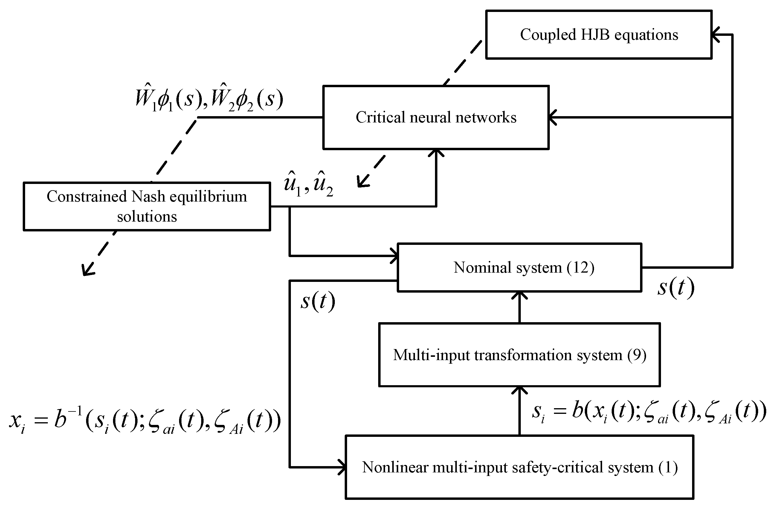
Combined with the previous content, the proposed multi-input safety-critical system structure diagram is shown in Figure 1.

Theorem 2.

Consider the system (9), the approximate optimal control strategy (33) and (34), and the weight tuning laws (37) and (38). Suppose that $\nabla {\varphi }_1$, $\nabla {\varphi }_2$, ${ϵ}_1$, $\nabla {ϵ}_1$, ${ϵ}_2$, $\nabla {ϵ}_2$, ${ϵ}_{B1}$, ${ϵ}_{B2}$ are all uniformly bounded. Assume that the Assumptions 1 and 2 hold. Then, the system state s, the neural network weight errors ${\tilde{W}}_1$, ${\tilde{W}}_2$ can be guaranteed to be UUB under the time-varying safety constraints and uncertain disturbances.

Proof of Theorem 2. 

See the Appendix A. □

Remark 4.

According to the result of Theorem 2, we can obtain that the neural network weight errors are UUB. According to formulas (33), (34), and (39), we can easily derive that, as ${\widehat{V}}_1(s)\to V_1^{*}(s)$, ${\widehat{V}}_2(s)\to V_2^{*}(s)$, then the control input ${\widehat{u}}_1\to u_1^{*}$, ${\widehat{u}}_2\to u_2^{*}$. That is, the control strategy can be approximately optimal.

Remark 5.

Compared with [35], this work considers a more complex and interesting constrained control problem, that is, the safety constraints change with time. In addition, we establish the coupled HJB equation to obtain the constrained optimal solution, so that the system state can complete convergence under the condition that the time-varying constraints are satisfied.

Remark 6.

In [34,36], the safety optimal control problem with external disturbance is considered, and the control scheme based on barrier transformation is designed. However, all of the external disturbances mentioned are known. In this work, the safety control problem with uncertain disturbance is further studied, and it is proved that the system state can complete convergence under the proposed control strategy.

4. Simulation

To prove the effectiveness of the proposed method, we give two nonlinear examples with time-varying safety constraints. In both cases, we observe that the system can satisfy the time-varying safety constraints.

4.1. Nonlinear System Example 1

Consider the affine nonlinear system as follows [30]:

$$\begin{array}{cc}\hfill \dot{x}=& \left[\begin{array}{c}{x}_2-2x_1\\ (-x_2-0.5x_1+0.25x_2{(cos(2x_1+2))}^2\\ +0.25x_2{(sin{(4x_1)}^2+2)}^2)\end{array}\right]+\left[\begin{array}{c}0\\ cos(2x_1+2)\end{array}\right]u_1+\hfill \\ \hfill & \left[\begin{array}{c}0\\ 4x_1^2+2\end{array}\right]u_2+\left[\begin{array}{c}0\\ cos(x_1)x_2\end{array}\right]d.\hfill \end{array}$$

(42)

In addition, $x={[x_1,x_2]}^T$ is the system state. One selects ${\alpha }_1={\alpha }_2=1,R_{11}=R_{12}=2,$ $R_{21}=R_{22}=1,Q_1=Q_2=[10;01]$. The initial system state is defined as $x_0={[2,2]}^T$. We choose $\phi (x)=x$ and $d(\phi (x))=p{x}_{1}sin{x}_2,p\in [-1,1]$. Similarly, we select $\delta (x)=x_{1}sin{x}_2$. Based on Formula (4) and (5), we define the time-varying parameters for $x_1$ as $l_1=-1,l_2=-0.6,{\vartheta }_1=-0.2,t_1=3,t_2=4,l_3=2.2,l_4=1.8,{\vartheta }_2=0.2$. We define the time-varying parameters for $x_2$ as $l_1=-2.8,l_2=-1.8,{\vartheta }_1=-0.5,$ $t_3=3,t_4=4,l_3=3,l_4=2,{\vartheta }_2=0.5$. Before 75 s, the persistence excitation condition is ensured by the probing noise. Since the effectiveness of the barrier transformation has been demonstrated in many previous works, we no longer compare our work with scenarios without safety constraints, but with scenarios with constant constraints.

We define the activation functions as

$$\begin{array}{c}\hfill {\varphi }_1(s)={\varphi }_2(s)={\left[s_1^2{s}_1{s}_2{s}_2^2\right]}^T.\end{array}$$

Meanwhile, the critic weight parameters are denoted as

$$\begin{array}{c}\hfill {\widehat{W}}_1={\left[{\widehat{\omega }}_{11}{\widehat{\omega }}_{12}{\widehat{\omega }}_{13}\right]}^T,{\widehat{W}}_2={\left[{\widehat{\omega }}_{21}{\widehat{\omega }}_{22}{\widehat{\omega }}_{23}\right]}^T.\end{array}$$

The critic parameters after 100 s converge to the value of ${\widehat{W}}_1=[-0.3921.7891.162]$, ${\widehat{W}}_2=[-1.8492.5900.142]$.

It is obtained from Figure 2 that the method of using constant constraints can satisfy constant constraints $(-1,2.2),(-2.8,3)$ in the process of system state convergence, but can not satisfy the time-varying constraints $({\zeta }_{a1},{\zeta }_{A1})$, $({\zeta }_{a2},{\zeta }_{A2})$. It can be seen that the trajectory of system state x obtained by the proposed method can converge to zero under the condition that time-varying safety constraints are satisfied. Figure 3 gives the evolution of the critic parameters for player 1. The evolution of the critic parameters for player 2 is shown in Figure 4. It can be seen that, according to the proposed tuning laws (37) and (38), the critic weight parameters converge to their ideal values. Figure 5 shows the state trajectories of the transformation system (9).

4.2. Nonlinear System Example 2

Consider the following nonlinear system of a single link robot arm:

$$\begin{array}{c}\hfill \dot{x}=\left[\begin{array}{c}{x}_2-2x_1\\ -5sin(x_1)-0.2x_2\end{array}\right]+\left[\begin{array}{c}0\\ 0.1\end{array}\right]u_1+\left[\begin{array}{c}0\\ 0.1\end{array}\right]u_2+\left[\begin{array}{c}0\\ 1\end{array}\right]d.\end{array}$$

(43)

In addition, $x={[x_1,x_2]}^T$ is the system state. One selects ${\alpha }_1=5,{\alpha }_2=1,R_{11}=R_{12}=2,$ $R_{21}=R_{22}=1,Q_1=Q_2=[50;05]$. The initial system state is defined as $x_0={[2,2]}^T$. Similarly, we choose $\phi (x)=x$, $d(\phi (x))=p{x}_{1}sin{x}_2,p\in [-1,1]$, and $\delta (x)=x_{1}sin{x}_2$. In this example, we apply the more complex time-varying safety constraints to the system state, where the constraints on the upper bounds of $x_1,x_2$ vary at 3 and 8 s, respectively, and the constraints on the lower bounds of $x_1$ and $x_2$ vary at 3 and 10 s, respectively. Define ${\lambda }_1=3$, ${\lambda }_2=18$ as the boundaries of the control inputs. Before 75 s, the persistence excitation condition is ensured by the probing noise.

We define the activation function as

$$\begin{array}{c}\hfill {\varphi }_1(s)={\varphi }_2(s)={\left[s_1^2{s}_1{s}_2{s}_2^2\right]}^T.\end{array}$$

Meanwhile, we denoted the critic weight parameters as

$$\begin{array}{c}\hfill {\widehat{W}}_1={\left[{\widehat{\omega }}_{11}{\widehat{\omega }}_{12}{\widehat{\omega }}_{13}\right]}^T,{\widehat{W}}_2={\left[{\widehat{\omega }}_{21}{\widehat{\omega }}_{22}{\widehat{\omega }}_{23}\right]}^T.\end{array}$$

The critic parameters after 100 s converge to the value of ${\widehat{W}}_1=$ [−1.319 0.249 −0.023], ${\widehat{W}}_2=$ [0.250 −1.113 0.658].

In Example 2, we further consider the case of input constraints. Figure 6 shows that the method using constant constraints cannot satisfy the time-varying safety constraints $({\zeta }_{a1},{\zeta }_{A1})$, $({\zeta }_{a2},{\zeta }_{A2})$ in the process of system state convergence, while the proposed method can ensure that the system state x converges under the time-varying safety constraints. The constrained control inputs are shown in Figure 7. The evolution of the critic parameters is given in Figure 8 and Figure 9. The transformation system state trajectories are shown in Figure 10.

5. Conclusions

For the affine nonlinear multi-input safety-critical systems with uncertain disturbances and time-varying safety constraints, a new adaptive learning algorithm based on the coupled HJB equations was proposed to solve the constrained optimal control problem. In order to satisfy the time-varying safety constraints, the novel barrier function and smooth safety boundary function were used to transform the safety-critical system into the transformation system without the time-varying safety constraints. The proposed barrier function solves the time-varying safety constraint problem which cannot be solved by the traditional constant constraint method. The influence of uncertain disturbances on the transformation system was dealt with reasonably by establishing the nominal system and disturbance-related term. In addition, two critic neural networks were used to learn the optimal solutions of the coupled HJB equations. The effectiveness of this method was verified by the theoretical proof. In addition, we test both the nonlinear system of the robotic arm and the numerical nonlinear example. Simulation results also verify the effectiveness of the proposed method.

References

1. Tee, K.P.; Ge, S.S.; Tay, E.H. Barrier Lyapunov Functions for the control of output-constrained nonlinear systems. IFAC Proc. Vol. 2013, 46, 449–455. [Google Scholar] [CrossRef]
2. Ames, A.D.; Coogan, S.; Egerstedt, M.; Notomista, G.; Sreenath, K.; Tabuada, P. Control barrier functions: Theory and applications. In Proceedings of the 18th European Control Conference (ECC), Saint Petersburg, Russia, 12 May 2020; pp. 3420–3431. [Google Scholar]
3. Wang, D.; He, H.; Liu, D. Adaptive Critic Nonlinear Robust Control: A Survey. IEEE Trans. Cybern. 2017, 47, 3429–3451. [Google Scholar] [CrossRef] [PubMed]
4. Wang, D.; Liu, D. Learning and guaranteed cost control with event-based adaptive critic implementation. IEEE Trans. Neural Netw. Learn. Syst. 2018, 29, 6004–6014. [Google Scholar] [CrossRef] [PubMed]
5. Vamvoudakis, K.G.; Lewis, F.L. Multi-player non-zero-sum games: Online adaptive learning solution of coupled Hamilton–Jacobi equations. Automatica 2011, 47, 1556–1569. [Google Scholar] [CrossRef]
6. Liu, D.; Xue, S.; Zhao, B.; Luo, B.; Wei, Q. Adaptive Dynamic Programming for Control: A Survey and Recent Advances. IEEE Trans. Syst. Man Cybern. Syst. 2021, 51, 142–160. [Google Scholar] [CrossRef]
7. El-Sousy, F.F.M.; Amin, M.M.; Al-Durra, A. Adaptive Optimal Tracking Control Via Actor-Critic-Identifier Based Adaptive Dynamic Programming for Permanent-Magnet Synchronous Motor Drive System. IEEE Trans. Ind. Appl. 2021, 57, 6577–6591. [Google Scholar] [CrossRef]
8. Liu, D.; Li, H.; Wang, D. Online Synchronous Approximate Optimal Learning Algorithm for Multi-Player Non-Zero-Sum Games With Unknown Dynamics. IEEE Trans. Syst. Man Cybern. 2014, 44, 1015–1027. [Google Scholar] [CrossRef]
9. Zhao, B.; Liu, D. Event-Triggered Decentralized Tracking Control of Modular Reconfigurable Robots Through Adaptive Dynamic Programming. IEEE Trans. Ind. Electron. 2020, 67, 3054–3064. [Google Scholar] [CrossRef]
10. Zhao, B.; Wang, D.; Shi, G.; Liu, D.; Li, Y. Decentralized Control for Large-Scale Nonlinear Systems With Unknown Mismatched Interconnections via Policy Iteration. IEEE Trans. Syst. Man Cybern. 2018, 48, 1725–1735. [Google Scholar] [CrossRef]
11. Wang, D.; Liu, D.; Li, H.; Ma, H. Neural-network-based robust optimal control design for a class of uncertain nonlinear systems via adaptive dynamic programming. Inf. Sci. 2014, 282, 167–179. [Google Scholar] [CrossRef]
12. Modares, H.; Lewis, F.L.; Jiang, Z.P. H tracking control of completely unknown continuous-time systems via off-policy reinforcement learning. IEEE Trans. Neural Netw. Learn. Syst. 2015, 26, 2550–2562. [Google Scholar] [CrossRef]
13. Wang, D.; He, H.; Liu, D. Improving the Critic Learning for Event-Based Nonlinear H Control Design. IEEE Trans. Cybern. 2017, 47, 3417–3428. [Google Scholar] [CrossRef] [PubMed]
14. Zhang, H.; Xi, R.; Wang, Y.; Sun, S.; Sun, J. Event-Triggered Adaptive Tracking Control for Random Systems With Coexisting Parametric Uncertainties and Severe Nonlinearities. IEEE Trans. Autom. Contr. 2022, 67, 2011–2018. [Google Scholar] [CrossRef]
15. Vamvoudakis, K.G.; Lewis, F.L. Online actor critic algorithm to solve the continuous-time infinite horizon optimal control problem. Automatica 2010, 46, 878–888. [Google Scholar] [CrossRef]
16. Li, J.; Ding, J.; Chai, T.; Lewis, F.L.; Jagannathan, S. Adaptive Interleaved Reinforcement Learning: Robust Stability of Affine Nonlinear Systems with Unknown Uncertainty. IEEE Trans. Neural Netw. Learn. Syst. 2022, 33, 270–280. [Google Scholar] [CrossRef] [PubMed]
17. Zhang, H.; Zhang, K.; Xiao, G.; Jiang, H. Robust Optimal Control Scheme for Unknown Constrained-Input Nonlinear Systems via a Plug-n-Play Event-Sampled Critic-Only Algorithm. IEEE Trans. Syst. Man Cybern. 2020, 50, 3169–3180. [Google Scholar] [CrossRef]
18. Wang, D.; Mu, C.; He, H.; Liu, D. Event-Driven Adaptive Robust Control of Nonlinear Systems With Uncertainties Through NDP Strategy. IEEE Trans. Syst. Man Cybern. 2017, 47, 1358–1370. [Google Scholar] [CrossRef]
19. Wei, Q.; Zhu, L.; Song, R.; Zhang, P.; Liu, D.; Xiao, J. Model-Free Adaptive Optimal Control for Unknown Nonlinear Multiplayer Nonzero-Sum Game. IEEE Trans. Neural Netw. Learn. Syst. 2022, 33, 879–892. [Google Scholar] [CrossRef]
20. Zhang, H.; Su, H.; Zhang, K.; Luo, Y. Event-Triggered Adaptive Dynamic Programming for Non-Zero-Sum Games of Unknown Nonlinear Systems via Generalized Fuzzy Hyperbolic Models. IEEE Trans. Fuzzy. Syst. 2019, 27, 2202–2214. [Google Scholar] [CrossRef]
21. Vamvoudakis, K.G.; Modares, H.; Kiumarsi, B.; Lewis, F.L. Game Theory-Based Control System Algorithms with Real-Time Reinforcement Learning: How to Solve Multiplayer Games Online. IEEE Contr. Syst. Mag. 2017, 37, 33–52. [Google Scholar]
22. Li, J.; Xiao, Z.; Li, P. Discrete-time Multi-player Games Based on Off-Policy Q-Learning. IEEE Access 2019, 7, 134647–134659. [Google Scholar] [CrossRef]
23. Su, H.; Zhang, H.; Jiang, H.; Wen, Y. Decentralized Event-Triggered Adaptive Control of Discrete-Time Nonzero-Sum Games Over Wireless Sensor-Actuator Networks With Input Constraints. IEEE Trans. Neural Netw. Learn. Syst. 2020, 31, 4254–4266. [Google Scholar] [CrossRef]
24. Song, R.; Wei, Q.; Zhang, H.; Lewis, F.L. Discrete-Time Non-Zero-Sum Games With Completely Unknown Dynamics. IEEE Trans. Cybern. 2021, 51, 2929–2943. [Google Scholar] [CrossRef]
25. Xue, S.; Luo, B.; Liu, D. Event-Triggered Adaptive Dynamic Programming for Zero-Sum Game of Partially Unknown Continuous-Time Nonlinear Systems. IEEE Trans. Syst. Man Cybern. 2020, 50, 3189–3199. [Google Scholar] [CrossRef]
26. Luo, B.; Yang, Y.; Liu, D. Policy Iteration Q-Learning for Data-Based Two-Player Zero-Sum Game of Linear Discrete-Time Systems. IEEE Trans. Cybern. 2021, 51, 3630–3640. [Google Scholar] [CrossRef] [PubMed]
27. Wang, W.; Chen, X.; Fu, H.; Wu, M. Model-Free Distributed Consensus Control Based on Actor–Critic Framework for Discrete-Time Nonlinear Multiagent Systems. IEEE Trans. Syst. Man Cybern. 2020, 50, 4123–4134. [Google Scholar] [CrossRef]
28. Qin, C.; Shang, Z.; Zhang, Z.; Zhang, D.; Zhang, J. Robust Tracking Control for Non-Zero-Sum Games of Continuous-Time Uncertain Nonlinear Systems. Mathematics 2022, 10, 1904. [Google Scholar] [CrossRef]
29. Song, R.; Lewis, F.L.; Wei, Q. Off-Policy Integral Reinforcement Learning Method to Solve Nonlinear Continuous-Time Multiplayer Nonzero-Sum Games. IEEE Trans. Neural Netw. Learn. Syst. 2017, 28, 704–713. [Google Scholar] [CrossRef] [PubMed]
30. Ming, Z.; Zhang, H.; Liang, L.; Su, H. Nonzero-sum differential games of continuous-Time nonlinear systems with uniformly ultimately ε-bounded by adaptive dynamic programming. Appl. Math. Comput. 2022, 430, 127248. [Google Scholar] [CrossRef]
31. Marvi, Z.; Kiumarsi, B. Safe reinforcement learning: A control barrier function optimization approach. Int. J. Robust Nonlinear Control 2021, 31, 1923–1940. [Google Scholar] [CrossRef]
32. Xu, J.; Wang, J.; Rao, J.; Zhong, Y.; Wang, H. Adaptive dynamic programming for optimal control of discrete-time nonlinear system with state constraints based on control barrier function. Int. J. Robust Nonlinear Control 2021, 32, 3408–3424. [Google Scholar] [CrossRef]
33. Liu, Y.J.; Lu, S.; Tong, S.; Chen, X.; Chen, C.P.; Li, D.J. Adaptive control-based Barrier Lyapunov Functions for a class of stochastic nonlinear systems with full state constraints. Automatica 2018, 87, 83–93. [Google Scholar] [CrossRef]
34. Yang, Y.; Ding, D.W.; Xiong, H.; Yin, Y.; Wunsch, D.C. Online barrier-actor-critic learning for H control with full-state constraints and input saturation. J. Franklin Inst. 2020, 357, 3316–3344. [Google Scholar] [CrossRef]
35. Yang, Y.; Vamvoudakis, K.G.; Modares, H. Safe reinforcement learning for dynamical games. Int. J. Robust Nonlinear Control 2020, 30, 3706–3726. [Google Scholar] [CrossRef]
36. Qin, C.; Wang, J.; Qiao, X.; Zhu, H.; Zhang, D.; Yan, Y. Integral Reinforcement Learning for Tracking in a Class of Partially Unknown Linear Systems with Output Constraints and External Disturbances. IEEE Access 2022, 10, 55270–55278. [Google Scholar] [CrossRef]
37. Qin, C.; Zhu, H.; Wang, J.; Xiao, Q.; Zhang, D. Event-Triggered Safe Control for the Zero-Sum Game of Nonlinear Safety-Critical Systems with Input Saturation. IEEE Access 2022, 10, 40324–40337. [Google Scholar] [CrossRef]
38. Hu, G. Observers for one-sided Lipschitz nonlinear systems. IMA J. Math. Control Inf. 2006, 23, 395–401. [Google Scholar] [CrossRef]
39. Modares, H.; Lewis, F.L.; Sistani, M. Online Solution of nonquadratic two-player zero-sum games arising in the H control of constrained input systems. Int. J. Adapt. Control 2014, 28, 232–254. [Google Scholar] [CrossRef]
40. Modares, H.; Lewis, F.L.; Naghibi-Sistani, M.B. Integral reinforcement learning and experience replay for adaptive optimal control of partially-unknown constrained-input continuous-time systems. Automatica 2014, 50, 193–202. [Google Scholar] [CrossRef]
Figure 1. The structure diagram of the proposed multi-input safety-critical system.
Mathematics 10 02744 g001
Figure 2. Evolution of the state x ( t ) by using the presented method and the method in [35].
Mathematics 10 02744 g002
Figure 3. Evolution of the critic estimates for player 1.
Mathematics 10 02744 g003
Figure 4. Evolution of the critic estimates for player 2.
Mathematics 10 02744 g004
Figure 5. Transformed system states using the presented method.
Mathematics 10 02744 g005
Figure 6. Evolution of the state x ( t ) by using the presented method and the method in [35].
Mathematics 10 02744 g006
Figure 7. Constrained control inputs of player 1 and player 2.
Mathematics 10 02744 g007
Figure 8. Evolution of the critic estimates for player 1.
Mathematics 10 02744 g008
Figure 9. Evolution of the critic estimates for player 2.
Mathematics 10 02744 g009
Figure 10. Transformed system states using the presented method.
Mathematics 10 02744 g010
Publisher’s Note: MDPI stays neutral with regard to jurisdictional claims in published maps and institutional affiliations.