On Robust Stability and Stabilization of Networked Evolutionary Games with Time Delays

Abstract

This paper investigates the robust stability and stabilization of networked evolutionary games (NEGs) with time delays. First, a mathematical model is presented to describe the dynamics of NEG with time-varying delays and disturbances. Second, an auxiliary system is constructed using the semi-tensor product of matrices and a dimension augmenting technique. Then, a verification condition of robust stability is derived. Third, in order to stabilize NEG to the Nash equilibrium, the robust stability problem is transformed into the robust stabilization problem. Moreover, an algorithm is proposed to design the stabilization controller. Finally, the validity of the results is verified by an example.

1. Introduction

In the 1940s, Von et al. [1] investigated game problems using a systematic mathematical approach. Subsequently, game theory has become a mathematical model used to study the decision-making behavior of players with rational thinking and learning ability. Note that interactions among numerous participants may not be evenly mixed. Specifically, players only interact with their neighbors, not with all players. Thus, interaction structures among players have attracted the attention of researchers. Numerous works [2,3,4] have used network graphs to describe the topology among players, with the nodes representing players and each edge connecting two interacting players. Based on strategy updating rule, the game evolves on the network architecture, which is called a networked evolutionary game (NEG) [5]. With the integration of disciplines, NEG provides a feasible framework for research into economics, sociology, and biology [6,7,8].

Finding equilibriums is one of the most important problems in game theory. Because the participants are capable of learning, their strategies evolve towards higher revenues [9,10]. Updating strategies in multiple directions makes it difficult to capture the profile dynamics. The Nash equilibrium [11] is a special combination of strategies in which each player unilaterally changes strategy without increasing revenues. Therefore, the stability of a profile at Nash equilibrium has great significance. It is worth noting that the Nash equilibrium may not be unique. If the NEG is expected to evolve to an optimal equilibrium, a feasible approach is to design the strategies of certain players to guide the strategy evolution of others. This is consistent with stabilization theory in control theory.

Players update their strategy by probing the information of their neighbors. However, certain factors that influence strategy selection should not be ignored. Among them, signal disturbances and information time delays are two prominent factors. For example, signals generated by an external device are disturbances, which interfere with the information interaction among players. The information delays caused by communication equipment can be regarded as bounded time-varying delays. In recent years, many articles have studied the influence of disturbances and time delays on game dynamics. For instance, Jimenez et al. [12,13] considered a game with bounded uncertain disturbances and obtained the effect of the disturbances on Nash equilibrium; Yuan et al. [14] designed an event-triggered strategy for nonlinear quadratic games with disturbances; Yang et al. [15] described the effect of stochastic disturbances on evolutionary game dynamics; Qin et al. [16] found that time delay affected the cooperation level of the prisoner’s dilemma game on a two-dimensional lattice; Stewart et al. [17] revealed that time delay could promote the emergence of cooperation in an NEG with a small number of players and strategies. In summary, disturbance and time delay make it difficult to analyze game dynamics. As far as we know, there are few results on the influence of the combination of disturbances and time delays on NEG dynamics, attracting us to further investigation.

NEG is a discrete system with finite value in essence. A matrix is an efficient mathematical tool in dealing with discrete systems. The semi-tensor product (STP) of matrices, proposed by Professor Cheng and his team [18,19], breaks the dimension limitation of traditional matrix products and enriches the research methods in the modern control field. In recent years, STP theory has been successfully applied in many fields, such as logical systems [20], finite games [21,22], graph theory [23], finite automatic machines [24], biological systems [25,26,27], and more. Based on the semi-tensor product of matrices, research on finite games has achieved fruitful results. For example, Cheng et al. [28] constructed the potential equation and presented the calculation method of the potential function; the orthogonal decomposition theorem was proposed in [29] based on the vector space structure; and the algebraic model of NEGs was established in [5] and their dynamic behavior was analyzed, including stability, controllability, and consistency. With the help of STP theory, it is possible to solve the robust stability problems of NEGs with time delays.

Compared with the previous works on the stability and stabilization of NEGs, the highlights of our findings are the following characteristics:

• Using STP of matrices and dimension augmenting technique, an auxiliary system is constructed to formulate the dynamics of NEGs with time delays and disturbances. The auxiliary system is a linear-like system. It reduces the difficulty of analyzing NEG dynamics with time-varying delays.
• Based on the auxiliary system, an explicit criterion is derived for robust stability. It is presented as a matrix and is easily verified by mathematical software such as Matlab.
• In order to stabilize NEG to the target equilibrium, the robust stability problem is transformed into the robust stabilization problem. Based on the auxiliary system, the necessary and sufficient condition is derived for set stabilization. Moreover, an algorithm is developed to design the set stabilization controller.

This paper is divided into the following sections. Section 2 introduces basic notation and the preliminaries of STP; Section 3 presents the NEG model and analyzes its robust stability; Section 4 discusses set stabilization; and Section 5 provides an example to illustrate the results. Finally, in Section 6 and Section 7, we close with a brief conclusion and point out several directions for future research.

2. Preliminaries

The basic notation used in the following section is introduced below.

(1)

${\mathbb{R}}_{m\times n}$ is the set of all $m\times n$ real matrices

(2)

${\mathbf{1}}_n:=\left[1,1,\cdots ,1\right]\in {\mathbb{R}}_{1\times n}$, ${\mathbf{0}}_n:=\left[0,0,\cdots ,0\right]\in {\mathbb{R}}_{1\times n}$

(3)

${\mathcal{D}}_k:=\{1,2,\cdots ,k\}$

(4)

$Co{l}_i\left(A\right)$($Ro{w}_i\left(A\right)$) denotes the i-th column (row) of matrix A

(5)

${\delta }_n^i:=Co{l}_i\left(I_n\right)$

(6)

${\Delta }_n:=\left\{{\delta }_n^i\right|i=1,2,\cdots ,n\}$

(7)

$L=[{\delta }_n^{i_1},{\delta }_n^{i_2},\cdots ,{\delta }_n^{i_n}]$ is a logical matrix, which is abbreviated as ${\delta }_n[i_1,i_2,\cdots ,i_n]$

(8)

${\mathcal{L}}_{m\times n}$ represents the set of $m\times n$-dimensional logical matrices

(9)

∘ denotes the Hadamard product of matrices

As STP is defined based on the Kronecker product, we first introduce the Kronecker product and then present the concept and properties of STP.

Definition 1

([19]). Let $X=\left[x_{ij}\right]\in {\mathbb{R}}_{m\times n},Y=\left[y_{ij}\right]\in {\mathbb{R}}_{p\times q}$. Then, the Kronecker product of X and Y is

$$X\otimes Y:=\left[\begin{array}{cccc}{x}_{11}Y& x_{12}Y& \cdots & x_{1n}Y\\ ⋮& ⋮& ⋮& ⋮\\ x_{m1}Y& x_{m1}Y& \cdots & x_{mn}Y\end{array}\right]\in {\mathbb{R}}_{mp\times nq}.$$

Definition 2

([19]). Let $X\in {\mathbb{R}}_{m\times n},Y\in {\mathbb{R}}_{p\times q}$. Then, the STP of X and Y is

$$X⋉Y:=(X\otimes I_{t/n})(Y\otimes I_{t/p}),$$

where $t=lcm(n,p)$ represents the least common multiple of n and p.

For simplicity of description, the products of all matrices are assumed as STP in the sequel and the symbol ”⋉” is omitted unless otherwise specified.

Identify elements $1,2,\cdots ,k\in {\mathcal{D}}_k$ as vector form ${\delta }_k^1,{\delta }_k^2,\cdots ,{\delta }_k^k\in {\Delta }_k$. There then exists a one-to-one correspondence from ${\mathcal{D}}_k$ to ${\Delta }_k$. Therefore, ${\mathcal{D}}_k$ and ${\Delta }_k$ can be regarded as the same set, where ${\Delta }_k$ is called the vector form of ${\mathcal{D}}_k$. Based on this, we introduce an important property to transform logical functions into algebraic forms in the following.

Lemma 1

([19]). For a mix-valued logical function $f(x_1,x_2,\cdots ,x_n):{\prod }_{i=1}^n{\mathcal{D}}_{k_i}\to {\mathcal{D}}_{k_0}$, there exists a unique matrix $M_f\in {\mathcal{L}}_{k_0\times k}$ such that

$$\begin{array}{c}\hfill f(x_1,x_2,\cdots ,x_n)=M_f{x}_1{x}_2\cdots x_n,\end{array}$$

where $x_i\in {\Delta }_{k_i},i=1,2,\cdots ,n$ and $k={\prod }_{i=1}^n{k}_i$. In addition, $M_f$ is called the structural matrix of f.

Lemma 2

([19]). Let $X\in {\mathbb{R}}_{t\times 1}$, $Y\in {\mathbb{R}}_{n\times 1}$, $x\in {\Delta }_n$, $y\in {\Delta }_l$, and $z\in {\Delta }_m$.

(1) 

Define $W_{[t,n]}={\delta }_{tn}[I_n\otimes {\delta }_t^1,I_n\otimes {\delta }_t^2,\cdots ,I_n\otimes {\delta }_t^t]$. Then, $YX=W_{[t,n]}XY$.

(2) 

Define $M_{[n,l,m]}={\mathbf{1}}_n\otimes I_l\otimes {\mathbf{1}}_m$ and ${\Phi }_n=Diag\{{\delta }_n^1,{\delta }_n^2,\cdots ,{\delta }_n^n\}$. Then, $M_{[n,l,m]}xyz=y$ and $xx={\Phi }_{n}x.$

Definition 3

([19]). The Khatri-Rao product of two matrices $X\in {\mathbb{R}}_{m\times n}$ and $Y\in {\mathbb{R}}_{l\times n}$ is

$$X\ast Y:=[Co{l}_1\left(X\right)\otimes Co{l}_1\left(Y\right),Co{l}_2\left(X\right)\otimes Co{l}_2\left(Y\right),\cdots ,Co{l}_n\left(X\right)\otimes Co{l}_n\left(Y\right)].$$

3. Formulation and Robust Stability Analysis of NEGs with Time Delays

In this section, we first present the model of NEG with time delays and disturbances. Then, the algebraic formulation is established to analyze the robust stability of the game.

3.1. Model Description

A normal form game, denoted by $\mathcal{G}$, consists of three parts:

(1)

The set of players $N=\{1,2,\cdots ,n\}$;

(2)

Each player has a strategy set $S_i=\{1,2,\cdots ,k_i\}$. The strategies of all players constitute a profile, and the set of a profile is denoted by $S={\prod }_{i=1}^n{S}_i$;

(3)

Each player has a payoff function, $c_i:S\to \mathbb{R}$.

A network graph $\mathbb{P}$ describes the topology among players, which consists of nodes and edges. Each edge is attached to an edge-related fundamental game, ${\mathcal{G}}_{ij}$, which is played by neighboring player i and player j. According to strategy updating rules (SURs), the game evolves on $\mathbb{P}$, namely, the NEG. Consider that the dynamics of an NEG are affected by the time-varying delay, $\tau \left(t\right)$, and external disturbance, ${\xi }_j\left(t\right)$, $j=1,2,\cdots ,n$. Specifically, $\tau \left(t\right)\in \{0,1,\cdots ,\eta \}$ depends on the profile, and ${\xi }_j\left(t\right)\in {\mathcal{D}}_q$ is generated by the following external disturbance system:

$$\begin{array}{c}\hfill \left\{\begin{array}{c}{\alpha }_i(t+1)=h_i({\alpha }_1\left(t\right),{\alpha }_2\left(t\right),\cdots ,{\alpha }_l\left(t\right)),i=1,2,\cdots ,l;\hfill \\ {\xi }_j\left(t\right)=g_j({\alpha }_1\left(t\right),{\alpha }_2\left(t\right),\cdots ,{\alpha }_l\left(t\right)),j=1,2,\cdots ,n,\hfill \end{array}\right.\end{array}$$

(1)

where ${\alpha }_i\left(t\right)\in {\mathcal{D}}_{{\varrho }_i}$ represents the states of system (1) at time t, ${\xi }_j\left(t\right)$ denotes the output of system (1) at time t, $h_i:{\Pi }_{\gamma =1}^l{\mathcal{D}}_{{\varrho }_{\gamma }}\to {\mathcal{D}}_{{\varrho }_i}$ and $g_j:{\Pi }_{\gamma =1}^l{\mathcal{D}}_{{\varrho }_{\gamma }}\to {\mathcal{D}}_q$ are logical functions, and $i=1,2,\cdots ,l,j=1,2,\cdots ,n$.

A detailed introduction of an NEG with time delays and disturbances is provided below.

Definition 4.

A disturbed NEG with time delays is denoted by ${\mathcal{G}}_d=(\mathbb{P},{\mathbb{G}}_E,\mathbb{F},\tau \left(t\right),\Xi \left(t\right))$, where

(1) 

$\mathbb{P}$ is a network graph with node set $N=\{1,2,\cdots ,n\}$ and edge set $E\subset N\times N$;

(2) 

${\mathbb{G}}_E=\left\{{\mathcal{G}}_{ij}\right|(i,j)\in E\}$ is a fundamental game set, where ${\mathcal{G}}_{ij}$ is an edge-related fundamental game played by players i and j;

(3) 

$\mathbb{F}=\{f_1,f_2,\cdots ,f_n\}$ is an SUR set, where $f_i$ is the SUR of player $i\in N$;

(4) 

$\tau \left(t\right)\in \{0,1,\cdots ,\eta \}$ is the time-varying delay that occurs when players receive information from others;

(5) 

$\Xi \left(t\right)=\{{\xi }_1\left(t\right),{\xi }_2\left(t\right),\cdots ,{\xi }_n\left(t\right)\}$ is a disturbance set.

Let ${\mathbb{N}}_i$ denote the neighbor set of player $i\in N$. The dynamics of ${\mathcal{G}}_d$ are formulated as

$$\begin{array}{c}\hfill x_i(t+1)=f_i(\left\{x_j(t-\tau \left(t\right))\right|j\in {\mathbb{N}}_i\},{\xi }_i\left(t\right)),i=1,2,\cdots ,n,t=0,1,\cdots ,\end{array}$$

(2)

where $x_i\left(t\right)\in S_i$ represents the strategy of player i at time t, $f_i:{\prod }_{j\in {\mathbb{N}}_i}{S}_j\times {\mathcal{D}}_q\to S_i$ is the SUR of player i. We denote by $(x_1\left(t\right),x_2\left(t\right),\cdots ,x_n\left(t\right))$ the profile of ${\mathcal{G}}_d$ at time t.

In addition, the overall payoff $c_i\left(t\right)$ of player $i\in N$ at time t is computed by

$$c_i\left(t\right)=\frac{{\sum }_{j\in {\mathbb{N}}_i}{c}_{ij}(x_i\left(t\right),x_j(t-\tau \left(t\right)),{\xi }_i\left(t\right))}{|{\mathbb{N}}_i|},$$

(3)

where $c_{ij}:S_i\times S_j\times {\mathcal{D}}_q\to \mathbb{R}$ denotes the payoff function of player i interacting with player j.

Subsequently, the dynamics (2) are converted into an algebraic formulation by the STP method.

3.2. Algebraic Formulation

First, we convert the strategies $1,2,\cdots ,k_i$ and disturbances $1,2,\cdots ,q$ into vector form, ${\delta }_{k_i}^1,{\delta }_{k_i}^2,\cdots ,{\delta }_{k_i}^{k_i}$ and ${\delta }_q^1,{\delta }_q^2,\cdots ,{\delta }_q^q$, respectively. Then, $x_i\left(t\right)\in {\Delta }_{k_i}$, and ${\xi }_i\in {\Delta }_q$, $i=1,2,\cdots ,n$. Applying Lemma 1, the dynamics (2) have the algebraic form as

$$\begin{array}{c}\hfill x_i(t+1)=F_i{⋉}_{j\in {\mathbb{N}}_i}{x}_j(t-\tau \left(t\right)){\xi }_i\left(t\right),i=1,2,\cdots ,n,\end{array}$$

(4)

where $F_i\in {\mathcal{L}}_{k_i\times {\prod }_{j\in {\mathbb{N}}_i}{k}_{j}q}$ is the structural matrix of $f_i.$

Next, we construct an auxiliary system for (2) using the dimension augmenting technique. A projection matrix $M_i$ is defined for player i as

$$\begin{array}{c}\hfill M_i=M_i^{\left[1\right]}\otimes M_i^{\left[2\right]}\otimes \cdots \otimes M_i^{\left[n\right]},i=1,2,\cdots ,n,\end{array}$$

(5)

where

$$\begin{array}{c}\hfill M_i^{\left[r\right]}=\left\{\begin{array}{c}{I}_{k_r},\mathrm{if}r\in {\mathbb{N}}_i;\hfill \\ {\mathbf{1}}_{k_r},\mathrm{otherwise},\hfill \end{array}\right.r=1,2,\cdots ,n.\end{array}$$

Let $x\left(t\right)={⋉}_{i=1}^n{x}_i\left(t\right)\in {\Delta }_k,z\left(t\right)={⋉}_{j=t-\eta }^{t}x\left(j\right)\in {\Delta }_{\overline{k}}$, where $k={\prod }_{i=1}^n{k}_i$ and $\overline{k}=k^{\eta +1}$. Using projection matrix (5), (4) can be further calculated as

$$\begin{array}{c}\hfill \begin{array}{ccc}{x}_i(t+1)& =& F_i{M}_{i}x(t-\tau \left(t\right)){\xi }_i\left(t\right)\hfill \\ & =& F_i{M}_i{M}_{[k^{\eta -\tau \left(t\right)},k,k^{\tau \left(t\right)}]}z\left(t\right){\xi }_i\left(t\right)\hfill \\ & :=& {\widehat{F}}_{i,\tau \left(t\right)}z\left(t\right){\xi }_i\left(t\right),i=0,1,\cdots ,n.\hfill \end{array}\end{array}$$

(6)

Considering the time-varying delay, there exists a structural matrix $M_{\eta }\in {\mathcal{L}}_{(\eta +1)\times k}$ such that

$$\tau \left(t\right)=M_{\eta }x\left(t\right).$$

Set ${\overline{F}}_i=[{\widehat{F}}_{i,0},{\widehat{F}}_{i,1},\cdots ,{\widehat{F}}_{i,\eta }]$. Then, (6) is equivalent to

$$\begin{array}{c}\hfill \begin{array}{ccc}{x}_i(t+1)& =& {\overline{F}}_i{M}_{\eta }x\left(t\right)z\left(t\right){\xi }_i\left(t\right)\hfill \\ & =& {\overline{F}}_i{M}_{\eta }{W}_{[\overline{k},k]}(I_{k^{\eta }}\otimes {\varphi }_k)z\left(t\right){\xi }_i\left(t\right)\hfill \\ & :=& {\tilde{F}}_{i}z\left(t\right){\xi }_i\left(t\right),i=0,1,\cdots ,n.\hfill \end{array}\end{array}$$

(7)

As for disturbances, let $\alpha \left(t\right)={⋉}_{i=1}^l{\alpha }_i\left(t\right)\in {\Delta }_{\omega }$ and $\xi \left(t\right)={⋉}_{j=1}^n{\xi }_j\left(t\right)\in {\Delta }_{q^n}$, where $\omega ={\Pi }_{i=1}^l{\varrho }_i$. According to Lemma 1, there exist two structural matrices $M_{h,i}\in {\mathcal{L}}_{\omega \times \omega }$ and $M_{g,j}\in {\mathcal{L}}_{q\times \omega }$ for $h_i$ and $g_j$, respectively, such that

$$\begin{array}{c}\hfill \left\{\begin{array}{c}{\alpha }_i(t+1)=M_{h,i}\alpha \left(t\right),i=1,2,\cdots ,l;\hfill \\ {\xi }_j\left(t\right)=M_{g,j}\alpha \left(t\right),j=1,2,\cdots ,n.\hfill \end{array}\right.\end{array}$$

(8)

Consequently, (7) is transformed as

$$\begin{array}{c}\hfill \begin{array}{ccc}{x}_i(t+1)& =& {\tilde{F}}_{i}z\left(t\right)M_{g,j}\alpha \left(t\right)\hfill \\ & =& {\tilde{F}}_i(I_{\overline{k}}\otimes M_{g,j})z\left(t\right)\alpha \left(t\right)\hfill \\ & :=& {\ddot{F}}_{i}z\left(t\right)\alpha \left(t\right),i=0,1,\cdots ,n.\hfill \end{array}\end{array}$$

(9)

Using the Khatri–Rao product of matrices, (8) and (9) can be converted into

$$\begin{array}{c}\hfill \alpha (t+1)=M_h\alpha \left(t\right),\end{array}$$

(10)

and

$$x(t+1)=Fz\left(t\right)\alpha \left(t\right),$$

where $M_h=M_{h,1}\ast M_{h,2}\ast \cdots \ast M_{h,n}\in {\mathcal{L}}_{\omega \times \omega }$ and $F={\ddot{F}}_1\ast {\ddot{F}}_2\ast \cdots \ast {\ddot{F}}_n\in {\mathcal{L}}_{k\times \omega \overline{k}}$. From $z(t+1)=x(t-\eta +1)x(t-\eta +2)\cdots x(t+1)$, we derive

$$\begin{array}{c}\hfill z(t+1)=Ez\left(t\right)\alpha \left(t\right),\end{array}$$

(11)

where $E\in {\mathcal{L}}_{\overline{k}\times \omega \overline{k}}.$ Let $\beta \left(t\right)=z\left(t\right)\alpha \left(t\right)\in {\Delta }_{\omega \overline{k}}$. An auxiliary system is constructed as

$$\begin{array}{c}\hfill \begin{array}{ccc}\beta (t+1)& =& z(t+1)\alpha (t+1)\hfill \\ & =& Ez\left(t\right)\alpha \left(t\right)M_h\alpha \left(t\right)\hfill \\ & =& E(I_{\omega \overline{k}}\otimes M_h)(I_{\overline{k}}\otimes {\Phi }_{\omega })\beta \left(t\right)\hfill \\ & :=& Q\beta \left(t\right),\hfill \end{array}\end{array}$$

(12)

where $Q=E(I_{\omega \overline{k}}\otimes M_h)(I_{\overline{k}}\otimes {\Phi }_{\omega })\in {\mathcal{L}}_{\omega \overline{k}\times \omega \overline{k}}.$

Remark 1.

Disturbance and time delay increase the difficulty of analyzing NEG dynamics. By dimension augmentation, the dynamic system (2) is equivalently converted into the algebraic system (12). System (12) is a linear-like system. With an initial state $\beta \left(0\right)$, the state of system (2) can be intuitively derived from system (12). Next, the dynamics of ${\mathcal{G}}_d$ are investigated based on system (12).

3.3. Robust Stability Analysis

Before analyzing the stability of ${\mathcal{G}}_d$, the concepts of robust Nash equilibrium and robust stability are described below.

Definition 5.

Consider the NEG ${\mathcal{G}}_d$. A profile $s^{*}=(s_1^{*},s_2^{*},\cdots ,s_n^{*})$ is a robust-Nash equilibrium if, for each player, $i\in N$,

$$\begin{array}{c}\hfill c_i(s_i^{*},s_{-i}^{*},{\xi }_i)\ge c_i(s_i,s_{-i}^{*},{\xi }_i),\forall s_i\in S_i,\forall {\xi }_i\in {\mathcal{D}}_q,\end{array}$$

(13)

where $s_{-i}^{*}=(s_1^{*},s_2^{*},\cdots ,s_{i-1}^{*},s_{i+1}^{*},\cdots ,s_n^{*}).$

It is assumed that $s^{*}$ is the robust-Nash equilibrium of ${\mathcal{G}}_d$ in the sequel. With an initial state $\beta \left(0\right)$, the profile of ${\mathcal{G}}_d$ at time t is denoted by $x(t;\beta (0\left)\right)$.

Definition 6.

The NEG ${\mathcal{G}}_d$ is robust stable at the robust-Nash equilibrium $s^{*}$ if there exists a positive integer T such that

$$\begin{array}{c}\hfill x(t;\beta \left(0\right))=s^{*},\forall \beta \left(0\right)\in {\Delta }_{\omega \overline{k}},\forall t\ge T.\end{array}$$

(14)

Similar to the concept of robust stability, the concept of set stability of a system (12) is defined. Given a nonempty set $\mathbb{V}\subset {\Delta }_{\omega \overline{k}}$, system (12) is said to be set stable at $\mathbb{V}$ if there exists an integer $\overline{T}$ such that

$$\beta (t;\beta \left(0\right))\in \mathbb{V},\forall \beta \left(0\right)\in {\Delta }_{\omega \overline{k}},\forall t\ge \overline{T}.$$

Note that as the disturbance system (1) is a finite-valued system, the evolutionary trajectory starting from initial $\alpha \left(0\right)\in {\Delta }_{\omega }$ can reach corresponding attractors of (1) in finite time. Assume that ${\gamma }_1,{\gamma }_2,\cdots ,{\gamma }_s$ are the attractors of (1). Let $\mathbb{L}=\{{\gamma }_1,{\gamma }_2,\cdots ,{\gamma }_s\}$,

$$z^{*}={\left(s^{*}\right)}^{\eta +1},$$

and

$$\begin{array}{c}\hfill \Gamma =\{z^{*}⋉{\gamma }_i|{\gamma }_i\in \mathbb{L}\}.\end{array}$$

(15)

Lemma 3.

The NEG ${\mathcal{G}}_d$ is robust stable at the robust-Nash equilibrium $s^{*}$ if and only if system (12) is set stable at Γ.

Proof. 

(Necessity) It is assumed that ${\mathcal{G}}_d$ is robust stable at $s^{*}$; then, there exists a positive integer T which makes Equation (14) valid. According to system (1), if $\beta \left(0\right)$ is given, $\alpha \left(0\right)$ and $\left\{\xi \right(t\left)\right|t=0,1,2\cdots \}$ are known. Therefore, the arbitrariness of $\left\{\xi \right(t\left)\right|t=0,1,2\cdots \}$ is equivalent to the arbitrariness of $\alpha \left(0\right)$. Set $\widehat{T}=T+\eta$. When $t\ge \widehat{T}$, we obtain $z\left(t\right)=z^{*}$ and $\alpha \left(t\right)\in \mathbb{L}$. Hence, $\beta \left(t\right)\in \Gamma ,\forall t\ge \widehat{T},\forall \beta \left(0\right)\in {\Delta }_{\omega \overline{k}}$. This implies that system (12) is set stable at $\Gamma$.

(Sufficiency) Assume that system (12) is set stable at $\Gamma$. Then, there exists an integer $\overline{T}$ such that $\beta \left(t\right)\in \Gamma$ holds for any $t\ge \overline{T}$ and any $\beta \left(0\right)\in {\Delta }_{\omega \overline{k}}$. Notice that $\beta \left(t\right)=z\left(t\right)⋉\alpha \left(t\right)$ is a one-to-one correspondence from ${\Delta }_{\overline{k}}⋉{\Delta }_{\omega }$ to ${\Delta }_{\omega \overline{k}}$. Thus, for any $t\ge \overline{T}$ and $\beta \left(0\right)\in {\Delta }_{\omega \overline{k}}$, we obtain $z\left(t\right)=z^{*}$ and $\alpha \left(t\right)\in \mathbb{L}$. It can be derived that $x(t;\beta \left(0\right))=s^{*},\forall t\ge \overline{T},\forall \beta \left(0\right)\in {\Delta }_{\omega \overline{k}}$. Therefore, ${\mathcal{G}}_d$ is robust stable at $s^{*}$.    □

Based on Lemma 3, we draw the following verification condition of the robust stability of ${\mathcal{G}}_d$.

Theorem 1.

The NEG ${\mathcal{G}}_d$ is robust stable at the robust-Nash equilibrium $s^{*}$ if and only if there exists an integer $\tilde{T}\le \omega \overline{k}$ such that

$$\begin{array}{c}\hfill \sum _{{\delta }_{\omega \overline{k}}^i\in \Gamma }Ro{w}_i\left(Q^{\tilde{T}}\right)={\mathbf{1}}_{\omega \overline{k}}.\end{array}$$

(16)

Proof. 

(Necessity) Suppose that ${\mathcal{G}}_d$ is robust stable at $s^{*}$. According to Lemma 3, system (12) is set stable at $\Gamma$. Therefore,

$$\beta \left(t\right)=Q^t\beta \left(0\right)\in \Gamma$$

holds for $\forall t\ge \tilde{T},\forall \beta \left(0\right)\in {\Delta }_{\omega \overline{k}}.$ Assume that $\beta \left(0\right)={\delta }_{\omega \overline{k}}^i$ and $\beta \left(\tilde{T}\right)={\delta }_{\omega \overline{k}}^{ϵ\left(i\right)}$. Clearly, ${\left(Q^{\tilde{T}}\right)}_{ϵ\left(i\right),i}=1$. From the arbitrariness of ${\delta }_{\omega \overline{k}}^i$, we derive that (16) holds. Notice that the state space of system (12) is finite; thus, $\tilde{T}\le \omega \overline{k}$.

(Sufficiency) Assume that (16) holds. Due to Q being a logical matrix, it can be derived that (16) remains available for any $t\ge \tilde{T}$. Then, $\beta (t;\beta (0\left)\right)\in \Gamma$ holds for any $t\ge \tilde{T}$ and any $\beta \left(0\right)\in {\Delta }_{\omega \overline{k}}$, which is equivalent to

$$z(t;\beta \left(0\right))=z^{*},\alpha \left(t\right)\in \mathbb{L},\forall t\ge \tilde{T},\forall \beta \left(0\right)\in {\Delta }_{\omega \overline{k}}.$$

Clearly, $x(t;\beta \left(0\right))=s^{*}$ holds for any $\beta \left(0\right)\in {\Delta }_{\omega \overline{k}}$ and any $t\ge \tilde{T}$. Consequently, ${\mathcal{G}}_d$ is robust stable at $s^{*}$.    □

4. Stabilization Analysis of NEGs with Time Delays and Disturbances

If ${\mathcal{G}}_d$ is expected to evolve to an optimal Nash equilibrium, a natural idea is to control certain players to guide the evolution. In this section, we present the model of ${\mathcal{G}}_d$ with control players and then investigate the stabilization problem.

4.1. Model Description

Considering ${\mathcal{G}}_d=(\mathbb{P},{\mathbb{G}}_E,\mathbb{F},\tau \left(t\right),\Xi \left(t\right))$, we divide the player set N into control player set $\mathbb{A}$ and state player set $\mathbb{B}$, where $\mathbb{A}\cup \mathbb{B}=N$ and $\mathbb{A}\cap \mathbb{B}=Ø$. There is a rule that state players are subject to their inherent SURs, and the strategies of control players can be designed. ${\mathcal{G}}_d$ with the above players distinction is denoted as ${\mathcal{G}}_{cd}$. Then, the dynamics of ${\mathcal{G}}_{cd}$ are formulated as

$$\begin{array}{c}\hfill a_i(t+1)={\vartheta }_i(\{a_{\rho }(t-\tau \left(t\right)),b_{\upsilon }(t-\tau \left(t\right))|\rho \in {{\mathbb{N}}_i}^A,\upsilon \in {{\mathbb{N}}_i}^B\},{\xi }_i\left(t\right)),i=1,2,\cdots ,\left|\mathbb{A}\right|,\end{array}$$

(17)

where $a_i\left(t\right)$ is the strategy of a state player i at time t, ${{\mathbb{N}}_i}^A$ (${{\mathbb{N}}_i}^B$) is the neighbor set of state players (control players) of player i, ${\vartheta }_i$ is the SUR of player i, and $b_v\left(t\right)$ is the strategy of control player v at time t.

Define $a\left(t\right)={⋉}_{i=1}^{\left|\mathbb{A}\right|}{a}_i\left(t\right)\in {\Delta }_{k_a}$, $\tilde{a}\left(t\right)={⋉}_{i=t-\eta }^{t}a\left(i\right)\in {\Delta }_{k_{\tilde{a}}}$, $b\left(t\right)={⋉}_{i=1}^{\left|\mathbb{B}\right|}{b}_i\left(t\right)\in {\Delta }_{k_b}$, and $\tilde{b}\left(t\right)={⋉}_{i=t-\eta }^{t}b\left(i\right)\in {\Delta }_{k_{\tilde{b}}}$. Similar to formulas (4)–(11), the algebraic formulations for ${\mathcal{G}}_{cd}$ can be derived as

$$\begin{array}{c}\hfill \tilde{a}(t+1)=\tilde{A}\tilde{b}\left(t\right)\tilde{a}\left(t\right)\alpha \left(t\right).\end{array}$$

(18)

Let $\chi \left(t\right):=\tilde{a}\left(t\right)\alpha \left(t\right)\in {\Delta }_{\omega k_{\tilde{a}}}.$ Referring to (12), an auxiliary system is derived for ${\mathcal{G}}_{cd}$ as

$$\begin{array}{c}\hfill \chi (t+1)=H\tilde{b}\left(t\right)\chi \left(t\right),\end{array}$$

(19)

where $H\in {\mathcal{L}}_{\omega k_{\tilde{a}}\times k_{\tilde{b}}\omega k_{\tilde{a}}}.$

4.2. Stabilization Analysis

Based on the auxiliary system (19), we investigate the stabilization problem of ${\mathcal{G}}_{cd}$. Before presenting the key results, we recall the concept of a control-invariant subset as follows: $\Lambda \subset {\Delta }_{\omega k_{\tilde{a}}}$ is a control-invariant subset of system (19) if there exist a time T and a control sequence ${\left\{\tilde{b}\left(i\right)\right\}}_{i=0}^t$ such that $\chi (t;\chi \left(0\right),{\{\tilde{b}\left(i\right)\}}_{i=0}^t)\in \Lambda$, $\forall t\ge T$. The union of all control-invariant subsets contained in $\Lambda$ is called the largest control-invariant subset, and is denoted by $I_m(\Lambda )$. An algorithm is provided to find the largest control-invariant subset of $\Lambda$ in Algorithm 1.

Algorithm 1: Find the largest control-invariant subset $I_m(\Lambda )$.

Step 1: Assume $\Lambda =\{{\delta }_{k_{\tilde{a}}}^{j_1},{\delta }_{k_{\tilde{a}}}^{j_2},\cdots ,{\delta }_{k_{\tilde{a}}}^{j_{\sigma }}\}$ and $j_1<j_2<\cdots <j_{\sigma }$. Set $C_{\Lambda }={\Sigma }_{i=1}^{\sigma }{\delta }_{k_{\tilde{a}}}^{j_i}$ and $U_{\Lambda }={\delta }_{k_{\tilde{a}}}[j_1,j_2,\cdots ,j_{\sigma }].$ Step 2: Let $i=0$, $V_0=\Lambda$. Step 3: If $C_{V_i}^{\top }\left({\Sigma }_{\lambda =1}^{k_{\tilde{b}}}H{\delta }_{k_{\tilde{b}}}^{\lambda }\right)U_{\Lambda }>{\mathbf{0}}_{|V_i|}$, set $I_m(\Lambda )=V_i$, stop. Step 4: Compute $V_i^c=\left\{{\delta }_{\omega k_{\tilde{a}}}^{j_i}\right|{\left[C_{V_i}^{\top }\left({\Sigma }_{\lambda =1}^{k_{\tilde{b}}}H{\delta }_{k_{\tilde{b}}}^{\lambda }\right)U_{\Lambda }\right]}_i=0\}$ and set $V_{i+1}=V_i\backslash V_i^c$. Step 5: If $V_{i=1}=Ø$, let $I_m(\Lambda )=Ø$, stop; otherwise, let $i=i+1$, return to Step 3 and repeat the calculation.

System (17) is said to be stabilized at $\lambda \in {\Delta }_{k_{\tilde{a}}}$, if there exist a positive integer $\widehat{T}$ and a control sequence ${\{\tilde{b}(i)\}}_{i=0}^t$ such that $\tilde{a}(t;\chi (0),{\{\tilde{b}(i)\}}_{i=0}^t)=\lambda ,\forall t\ge \widehat{T},\forall \chi (0)\in {\Delta }_{\omega k_{\tilde{a}}}.$ Assume $s^{*}$ is the robust-Nash equilibrium of system (17). Similar to (15), we construct $\tilde{\Gamma }\subset {\Delta }_{\omega k_{\tilde{a}}}$. With a nonempty set $\Lambda \subset {\Delta }_{\omega k_{\tilde{a}}}$, system (19) is set stabilized at $\Lambda$ if there exist a positive integer $\check{T}$ and a control sequence ${\{\tilde{b}(i)\}}_{i=0}^t$ such that $\chi (t;\chi (0),{\{\tilde{b}(i)\}}_{i=0}^t)\in \Lambda ,\forall t\ge \check{T},\forall \chi (0)\in {\Delta }_{\omega k_{\tilde{a}}}.$

Next, the robust stabilization problem of ${\mathcal{G}}_{cd}$ is transformed into the set stabilization problem of system (19).

Theorem 2.

Considering ${\mathcal{G}}_{cd}$, the following statements are equivalent.

(1) 

${\mathcal{G}}_{cd}$ is stabilized at the robust-Nash equilibrium $s^{*}$ under control.

(2) 

System (19) is set stabilized at $\tilde{\Gamma }$.

(3) 

There exists a positive integer $ϵ\le \omega k_{\tilde{a}}$ such that

$$\begin{array}{c}\hfill C_{I_m\left(\tilde{\Gamma }\right)}^{\top }{\left({\Sigma }_{\lambda =1}^{k_{\tilde{b}}}H{\delta }_{k_{\tilde{b}}}^{\lambda }\right)}^{ϵ}>{\mathbf{0}}_{\omega k_{\tilde{a}}}.\end{array}$$

(20)

Proof. 

$\left(1\right)\Rightarrow \left(2\right):$ Similar to the proof of Lemma 3, it is easy to know that $\left(1\right)$ is equivalent to $\left(2\right)$.

$(2)\Rightarrow (3):$ Assume that system (19) is set stabilized at $\tilde{\Gamma }$. Then, there exist an integer $T_1$ and a control sequence ${\{\tilde{b}(i)\}}_{i=0}^t$ such that $\chi (t;\chi (0),{\{\tilde{b}(i)\}}_{i=0}^t)\in \tilde{\Gamma },\forall t\ge T_1,\forall \chi (0)\in {\Delta }_{\omega k_{\tilde{a}}}.$ Next, we prove that system (19) is stabilized at $I_m(\tilde{\Gamma })$ by contradiction. Suppose that there exist $\chi (0)={\delta }_{\omega k_{\tilde{a}}}^j$ and $t_1>T_1$ such that $\chi (t_1;{\delta }_{\omega k_{\tilde{a}}}^j,{\{\tilde{b}(i)\}}_{i=0}^{t_1})\notin I_m(\tilde{\Gamma })$. Considering that system (19) is set stabilized at $\tilde{\Gamma }$, we derive $\chi (t_1;{\delta }_{\omega k_{\tilde{a}}}^j,{\{\tilde{b}(i)\}}_{i=0}^{t_1})\in \tilde{\Gamma }\backslash I_m(\tilde{\Gamma }).$ This is contrary to $I_m(\tilde{\Gamma })$ being the largest control-invariant subset of $\tilde{\Gamma }$. Therefore, system (19) is set stabilized at $I_m(\tilde{\Gamma })$. Then, there exist an integer $T_2\le \omega k_{\tilde{a}}$ and a control sequence ${\{\tilde{b}(i)\}}_{i=0}^t$ such that $\chi (t;\chi (0),{\{\tilde{b}(i)\}}_{i=0}^t)\in I_m(\tilde{\Gamma })$ holds for any $t\ge T_2$ and any $\chi (0)\in {\Delta }_{\omega k_{\tilde{a}}}$. Consequently, (20) holds.

$(3)\Rightarrow (2):$ Suppose that (20) holds. This implies that for any $\chi (0)\in {\Delta }_{\omega k_{\tilde{a}}}$, there exists a control sequence ${\{\tilde{b}(i)\}}_{i=0}^{ϵ}$ such that $\chi (ϵ;\chi (0),{\{\tilde{b}(i)\}}_{i=0}^{ϵ})\in I_m(\tilde{\Gamma }).$ According to the definition of the largest control-invariant subset, we know that for any $\chi (0)\in {\Delta }_{\omega k_{\tilde{a}}}$ there exists ${\{\tilde{b}(i)\}}_{i=0}^t$ such that $\chi (t;\chi (0),{\{\tilde{b}(i)\}}_{i=0}^t)\in I_m(\tilde{\Gamma })\subset \tilde{\Gamma },\forall t\ge ϵ.$ Consequently, system (19) is set stabilized at $\tilde{\Gamma }$.    □

Algorithm 2 is presented below to design $\tilde{b}\left(t\right)={\rm Y}\chi \left(t\right)$ in order to ensure that ${\mathcal{G}}_{cd}$ is stabilized at the robust-Nash equilibrium.

Algorithm 2: Design control matrix ${\rm Y}$ such that $\tilde{b}(t)={\rm Y}\chi (t)$ and $\chi (t;\chi (0),\tilde{b}(t))\in \tilde{\Gamma }$.

Step 1: Let $V_0=I_m(\tilde{\Gamma })$. Assume $C^i={\mathbf{0}}_{k_{\tilde{b}}\times \omega k_{\tilde{a}}},i=1$. Step 2: For $j=1,2,\cdots ,k_{\tilde{b}},r=1,2,\cdots ,\omega k_{\tilde{a}}$, if $Co{l}_{(j-1)\omega k_{\tilde{a}}+r}(H)\in V_{i-1}$, set ${\left[C^i\right]}_{jr}=1.$ Step 3: Calculate $K_i=\{{\delta }_{\omega k_{\tilde{a}}}^r|Co{l}_r(C^i)\ne {\mathbf{0}}_{k_{\tilde{b}}}^{\top }\}$. Set $V_i=K_i\backslash {\bigcup }_{j=0}^{i-1}{V}_j$. Step 4: If $V_i=Ø$, there is no ${\rm Y}$. Stop the calculation. Step 5: If ${\bigcup }_{j=0}^i{V}_j={\Delta }_{\omega k_{\tilde{a}}}$, set $i^{*}=i$; otherwise, set $i=i+1$ and go back to Step 2. Step 6: Set $C^0=C^1$. ${\rm Y}$ is designed as $Co{l}_r({\rm Y})\in \{\varphi \in {\Delta }_{k_{\tilde{b}}}|\varphi \circ Co{l}_r(C^j)=\varphi \},$ where ${\delta }_{\omega k_{\tilde{a}}}^r\in V_j,j=0,1,\cdots ,i^{*}.$ Stop.

5. Example

5.1. Model Description

Consider an NEG ${\mathcal{G}}_d^1=(\mathbb{P},{\mathbb{G}}_E,\mathbb{F},\tau \left(t\right),\Xi \left(t\right))$ which has three players, $N=\{1,2,3\}$, and a strategy set $S_1=S_2=S_3=\{1,2\}$. The detailed information is as follows.

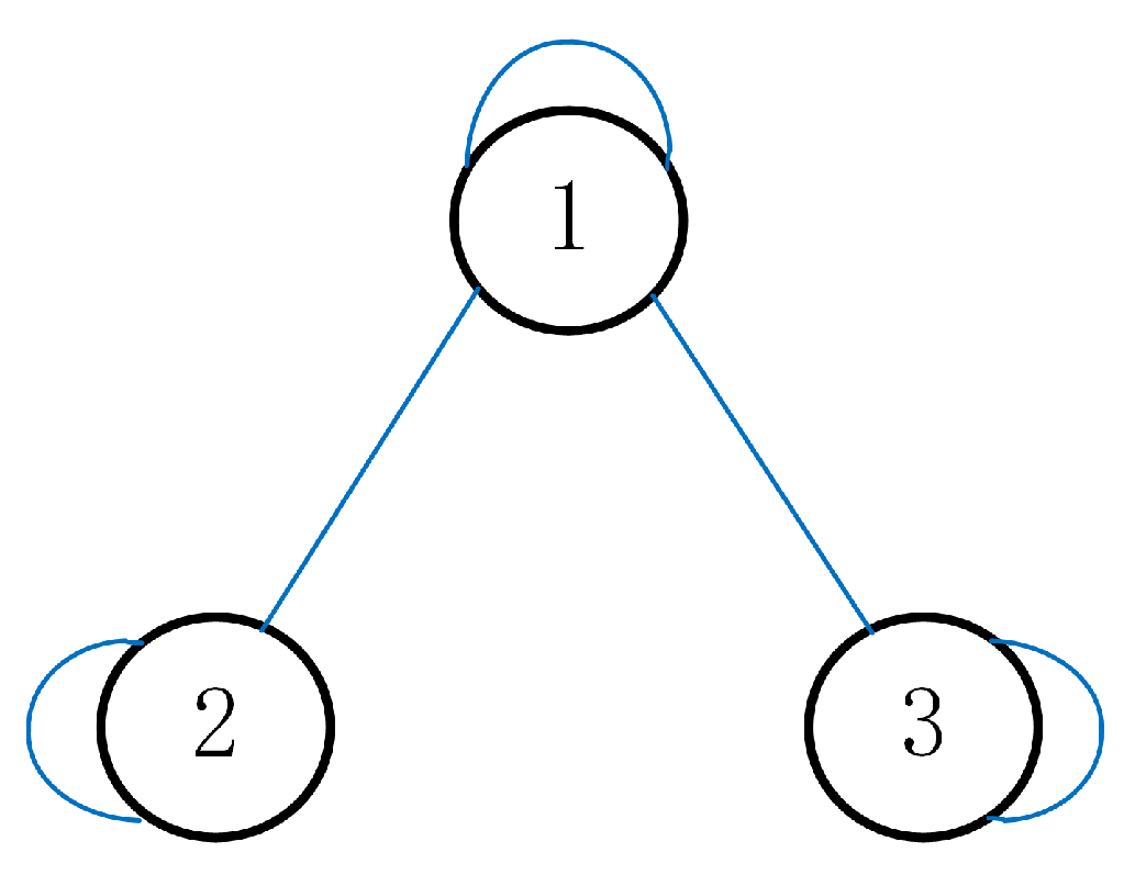
(1)

The network graph $\mathbb{P}$ is shown in Figure 1.

(2)

There are two edge-related fundamental games, ${\mathcal{G}}_{12}$ and ${\mathcal{G}}_{13}$; the payoff matrices are provided in

Table 1. Payoff Matrix of ${\mathcal{G}}_{12}$.

$\mathit{C}|\mathit{S}{\mathcal{D}}_2$	1111	1112	1121	1122	1211	1212	1221	1222	2111	2112	2121	2122	2211	2212	2221	2222
$c_1$	1	2	2	1	1	1	0	1	2	0	0	3	3	0	4	2
$c_2$	0	1	2	1	0	0	2	0	1	2	1	0	0	1	2	4

and

Table 2. Payoff Matrix of ${\mathcal{G}}_{13}$.

$\mathit{C}|\mathit{S}{\mathcal{D}}_2$	1111	1112	1121	1122	1211	1212	1221	1222	2111	2112	2121	2122	2211	2212	2221	2222
$c_1$	1	2	2	0	2	0	1	0	4	1	4	1	2	0	1	4
$c_3$	1	0	1	4	1	1	2	3	0	0	1	0	1	3	1	2

.

(3)

Imitating the strategy of the neighbor who has the optimal payoff is the SUR of each player, namely,

$$\begin{array}{c}\hfill x_i(t+1)=\left\{\begin{array}{c}{x}_i\left(t\right),\mathrm{if}{c}_i\left(t\right)\ge c_j\left(t\right),j\in {\mathbb{N}}_i;\hfill \\ x_j\left(t\right),\mathrm{if}{c}_i\left(t\right)<c_j\left(t\right),j\in {\mathbb{N}}_i.\hfill \end{array}\right.\end{array}$$

(4)

$\tau \left(t\right)=[0,1,0,1,1,1,0,0]x\left(t\right)$.

(5)

The external disturbance system is

$$\begin{array}{c}\hfill \left\{\begin{array}{c}\alpha (t+1)=M_h\alpha \left(t\right);\hfill \\ {\xi }_j\left(t\right)=M_{g,j}\alpha \left(t\right),j=1,2,3,\hfill \end{array}\right.\end{array}$$

where $M_h={\delta }_4[1,3,4,1]$, $M_{g,1}={\delta }_2[1,2,1,2]$, $M_{g,2}={\delta }_2[2,1,1,2]$, $M_{g,3}={\delta }_2[1,1,2,2]$.

The dynamics of ${\mathcal{G}}_d^1$ are formulated as

$$\begin{array}{c}\hfill \left\{\begin{array}{c}{x}_1(t+1)=f_1(x_1(t-\tau \left(t\right)),x_2(t-\tau \left(t\right)),x_3(t-\tau \left(t\right)),{\xi }_1\left(t\right)),\hfill \\ x_2(t+1)=f_2(x_1(t-\tau \left(t\right)),x_2(t-\tau \left(t\right)),{\xi }_2\left(t\right)),\hfill \\ x_3(t+1)=f_3(x_1(t-\tau \left(t\right)),x_3(t-\tau \left(t\right)),{\xi }_3\left(t\right)).\hfill \end{array}\right.\end{array}$$

5.2. Robust Stability Analysis

Using the semi-tensor product of matrices, the auxiliary system is constructed as

$$\beta (t+1)=Q\beta \left(t\right),$$

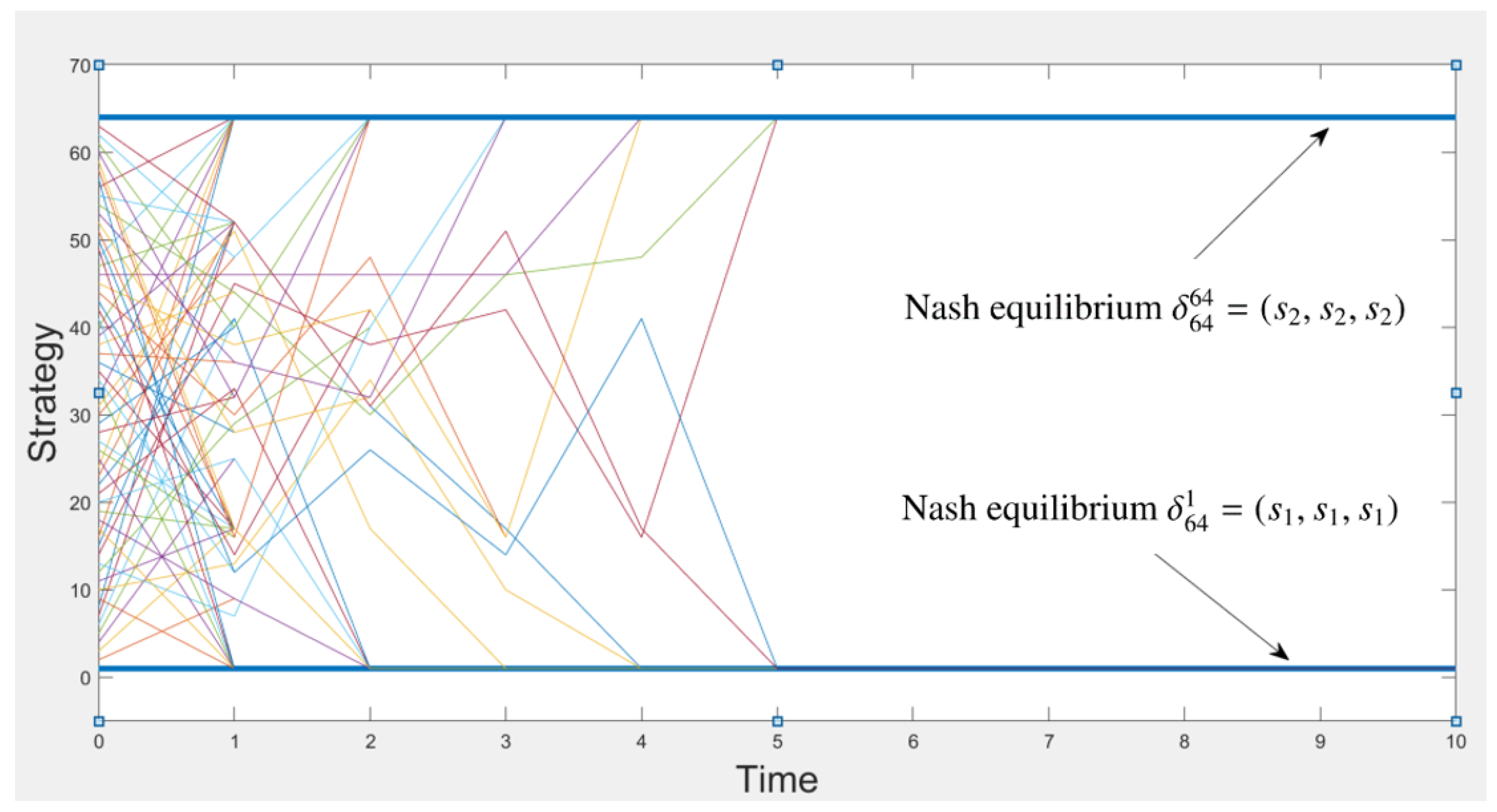
where $Q\in {\mathcal{L}}_{256\times 256}.$ The evolutionary trajectory of ${\mathcal{G}}_d^1$ is described by Figure 2, from which we can see that the trajectories initialized from any profiles are stabilized at two equilibriums, $(s_1,s_1,s_1)$ and $(s_2,s_2,s_2)$.

A calculation shows that ${\delta }_4^1$ is the unique fixed point of the disturbance system. We can find an integer $T=5$ such that $Ro{w}_1\left(Q^5\right)+Ro{w}_{253}\left(Q^5\right)={\mathbf{1}}_{256}$. Clearly, $\Gamma =\{{\delta }_{64}^1⋉{\delta }_4^1,{\delta }_{64}^{64}⋉{\delta }_4^1\}$. According to Theorem 1, ${\mathcal{G}}_d^1$ is robust stable at Nash equilibriums $(s_1,s_1,s_1)$ and $(s_2,s_2,s_2)$.

5.3. Robust Stabilization Analysis

Assuming that $(s_2,s_2,s_2)$ is an optimal Nash equilibrium, we consider the control problem. Let player 1 be a control player and players 2 and 3 be state players; ${\mathcal{G}}_d^1$ with player classification is rewritten as ${\mathcal{G}}_{cd}^1$. The dynamics of ${\mathcal{G}}_{cd}^1$ are described as

$$\begin{array}{c}\hfill \left\{\begin{array}{c}{a}_1(t+1)={\vartheta }_1(b(t-\tau \left(t\right)),a_1(t-\tau \left(t\right)),{\xi }_2\left(t\right)),\hfill \\ a_2(t+1)={\vartheta }_2(b(t-\tau \left(t\right)),a_2(t-\tau \left(t\right)),{\xi }_3\left(t\right)),\hfill \end{array}\right.\end{array}$$

where ${\vartheta }_1=f_2$, ${\vartheta }_2=f_3$, and the time delay is $\tau \left(t\right)=[0,1,0,1]a\left(t\right)$.

We intend to control player 1 to steer ${\mathcal{G}}_{cd}^1$ to be stabilized at $(s_2,s_2)$. According to (18) and (19), an auxiliary system is constructed as $\chi (t+1)=H\tilde{b}(t)\chi (t),$ where $H\in {\mathcal{L}}_{64\times 256},$ and $\tilde{\Gamma }=\{{\delta }_{16}^{16}⋉{\delta }_4^1\}:=\{{\delta }_{64}^{61}\}$. Clearly, $I_m(\tilde{\Gamma })={\delta }_{64}^{61}$. A calculation shows $Ro{w}_{61}{({\sum }_{i=1}^{4}H{\delta }_4^i)}^5>{\mathbf{0}}_{64}$. Per Theorem 2, $\chi (t)$ can be steered to $\tilde{\Gamma }$.

According to Algorithm 2, one feasible choice of ${\rm Y}$ is ${\rm Y}={\delta }_4[4,4,4,\cdots ,4,4,4]\in {\mathcal{L}}_{4\times 64}$. Under the controller $\tilde{b}(t)={\rm Y}\chi (t)$, we derive that $\chi (t;\chi (0),{\{\tilde{b}(i)\}}_{i=0}^t)={\delta }_{64}^{61}$ holds for any $t\ge 5$ and any $\chi (0)\in {\Delta }_{64},$ and then ${\mathcal{G}}_{cd}^1$ is stabilized at ${\delta }_{16}^{16}=(s_2,s_2)$.

6. Problems

The method presented in this paper is helpful for analyzing the robust stability of NEGs with disturbances and time delays. An efficient algorithm is provided to design the stabilization controller such that the NEG can be stabilized at the robust-Nash equilibrium. However, two problems have not been solved.

Problem 1.

According to the results obtained in this paper, the stability of ${\mathcal{G}}_d$ at $s^{*}$ is equivalent to the stability at Γ. This implies that the Nash equilibrium remains affected by disturbances. Is there a way to keep the Nash equilibrium from being disturbed?

Problem 2.

The design of the controller is affected by the disturbance as well. Is it possible to find a method by which a controller can be designed that is not affected by the disturbance?

7. Conclusions

In this paper, the robust stability and stabilization of NEGs with time delays have been studied. The evolutionary trajectory of the NEG is difficult to track because of the time delays and disturbances. Two higher-order auxiliary systems have been established using the dimension augmenting technique in order to resolve these difficulties. Unlike continuous systems, the effect of time delay on discrete systems can be eliminated via the dimension augmenting technique. In this case, the robust stability of the NEG can be investigated just as for non-delay systems. Based on the auxiliary system, necessary and sufficient conditions for robust stability and stabilization, respectively, have been obtained. Moreover, an algorithm has been proposed to design the state-feedback controller. Finally, the validity of the conclusions has been verified by an example.