Mesh Processing for Snapping Feature Points and Polylines in Orebody Modeling

Abstract

The 3D refinement modeling of the orebody provides an important guarantee for the estimation of the resources and reserves of an ore deposit. Implicit modeling techniques can effectively improve the efficiency of orebody modeling and facilitate the dynamic updating of the model. However, due to the problems of ambiguity and missing features during implicit surface interpolation and implicit surface reconstruction, the mesh models of orebodies obtained by means of implicit modeling techniques do not easily snap to the geological feature points and feature polylines obtained based on geological sampling data. In essence, all models are inaccurate, but geological sampling data are very useful and valuable, which should be accurately and effectively involved in the orebody modeling process. This would help to improve the reliability of resource estimation and mining design. The main contribution of this paper is the proposal of a method for accurately snapping orebody features after implicit modeling. This method enables the orebody model to snap accurately to the geological feature points and feature polylines and realizes the accurate clipping of the model boundary. We tested the method with real geological datasets. The results showed that the method is applicable and effective when the geological feature points and feature polylines are close to those of the orebody mesh model and the shape trend changes little, and the model can thus meet the practical application requirements of mines.

1. Introduction

Since the 21st century, with the development of earth science and computer science, 3D digital modeling technology [1] has been gradually introduced into the field of geology. The combination of mathematical geology [2] and computer technology has provided a new way for 3D geological modeling to be applied in mining development. As a kind of important geological bodies with special economic and social value, the construction of 3D orebody models has provided the basis for promoting the process of mine digitization [3] and intelligence [4], and obtaining high-precision models reflecting the spatial shape of the orebody is an important guarantee for the estimation of the resource and reserves of an ore deposit.

Due to the complexity [5] of the spatial shape of orebodies and the limitations of 3D orebody modeling technology, the orebody models built by geological engineers using most of the current mainstream mining modeling software [6,7,8,9] are often unable to meet the requirements of rapid and refined modeling [10], which greatly affects the efficiency and reliability of mine resource reserve estimation and mining design. Therefore, the problem of the 3D refinement modeling of orebodies has become an important bottleneck [11] restricting the digital and intelligent development of mines.

According to the different processes used for the 3D simulation of orebody surface structure, modeling methods can be summarized into explicit modeling [12], implicit modeling [13], and hybrid modeling [14] (i.e., explicit-implicit integration modeling). Implicit orebody modeling technology is the product of the combination of mathematical geology and computer technology. It generates more complete sample data from sparse orebody sampling data through spatial interpolation and uses an interpolation function to express the surface model of the orebody. With the help of surface reconstruction technology, the 3D visual model of the orebody is automatically generated. This approach is favored by experts and scholars in the field of mining modeling because it has the advantages of high automation and dynamic simulation [15]. Among its applications, Zhong et al. [16,17,18,19] conducted a large amount of theoretical and applied research on key technical problems such as geological rule constraints, surface interpolation functions, and implicit surface reconstruction methods in implicit orebody modeling.

In practical applications, for any modeling method, the orebody models built using sparse sampling data are essentially inaccurate. However, sampling data are very useful and relatively accurate [20], providing an important basis for mining development. It should be ensured that the sampling data can accurately and effectively participate in the orebody modeling process. 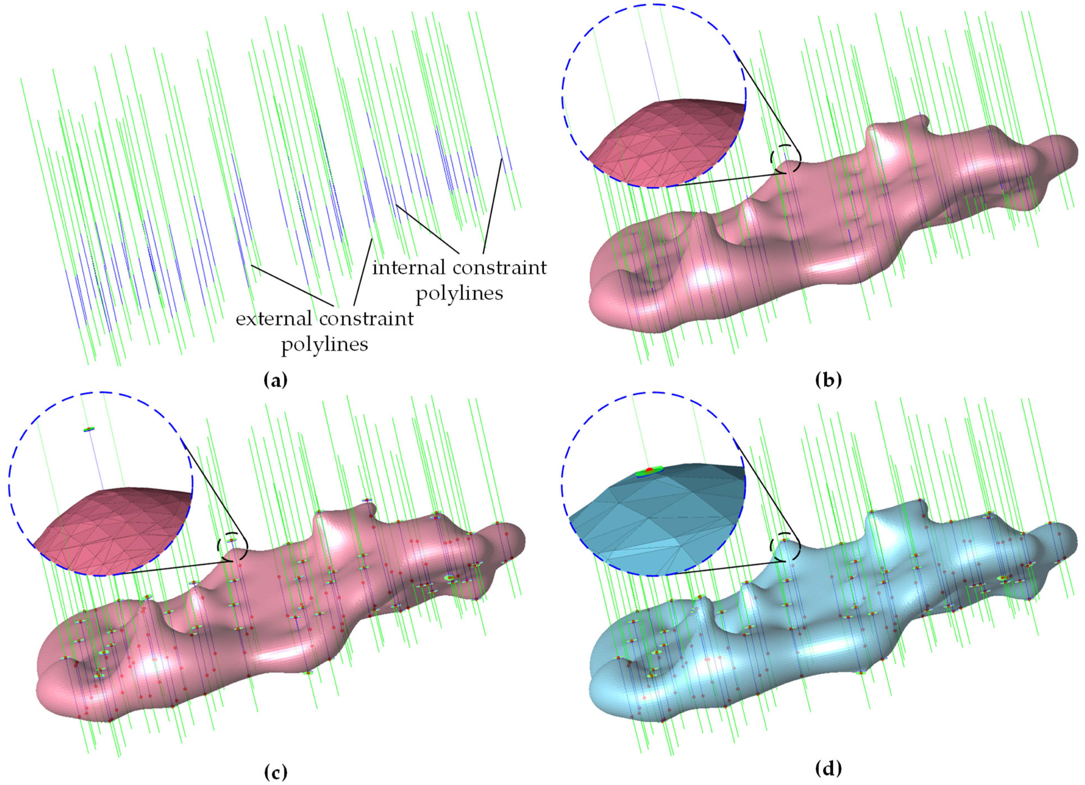As an important achievement in drilling engineering and geological logging, borehole data contain particularly valuable mine geological information, such as the borehole location, sample lithology, and sample element grade [21]. Because borehole data are discrete, the boundary contact points between orebodies and non-mineral rock bodies can be accurately captured after sample combination. It is worth noting that geological interpretation polylines (such as orebody contour polylines), delineated based on the borehole data and prior knowledge, can also be considered to be relatively accurate. From the perspective of model features, geological interpretation points and geological interpretation polylines, including boundary contact points and orebody contour polylines, can be regarded as the feature points and feature polylines of the model. They can also be transformed into constraint points and constraint polylines required for implicit modeling.

Theoretically, according to the different constraints of the spatial constraint data set, the results of implicit modeling can approach the real shape of the orebody model infinitely, in order to establish a more accurate orebody model in line with the constraint data. Because the orebody constraint data are relatively sparse, the mesh model obtained using implicit modeling technology often does not fully conform to the constraint data and features of the model. On the one hand, the implicit modeling results are not completely consistent with the orebody surface constraint data, and there is a gap between the generated model and the constraint points or constraint polylines. On the other hand, the implicit modeling results are inconsistent with the actual boundary of the orebody model, and the generated model boundary is greater than or less than the actual boundary of the orebody model. Generally, a refined 3D structure model can be considered a seamless model with the accurate snapping of feature data and the strict matching of model boundaries [22,23]. In general, an orebody model based on implicit modeling technology should exhibit no gaps with the constraint points and constraint polylines, and the boundary contour of the model should be topologically consistent with the actual boundary constraint polylines of the orebody model.

Based on the analysis of the modeling process, there are two main reasons why the implicit modeling results can not accurately snap to the features of the model. One is the implicit surface interpolation process [24], and the other is the implicit surface reconstruction process [25]. The accurate interpolation of constraint points can be realized in the process of implicit surface interpolation. However, the constraint points are discrete, and ambiguous constraint points can easily appear [26], which may lead to interpolation errors or some constraint points being unable to participate in the interpolation process. In addition, in this process, the exact interpolation of constraint points is easy to achieve, but the exact interpolation of constraint polylines is difficult to achieve. In the process of implicit surface reconstruction, the mesh model obtained via surface reconstruction methods (such as the iso-surface extraction method [27]) generally finds it difficult to accurately capture the given constraint points and constraint polylines [28,29]. Although there are some feature reconstruction methods for mesh models [30,31,32], there are still some problems with the application of this approach to orebody models, which need to be further improved.

With the aim of solving the problem of accurately snapping the feature data of an orebody model, we have mainly analyzed the process of implicit surface reconstruction. We have mainly adopted the method of iso-surface extraction for surface reconstruction. Generally, there are two ways to ensure that the extracted iso-surface snaps to the given feature points and polylines, using pre-processing and post-processing, respectively. The pre-processing of model snapping involves snapping the feature points and polylines directly during the process of iso-surface extraction. To preserve model features, some scholars have improved the iso-surface extraction algorithm. Xi et al. [33] proposed a region-growing-based iso-surface extraction algorithm that can generate high-quality curvature-adaptive meshes and preserve sharp features. Cebral et al. [34] extended the application of the surface merging algorithm based on the extraction of iso-surfaces from a distance map defined on an adaptive background grid to mesh surfaces with sharp edges and corners.

The post-processing of model snapping involves snapping the obtained mesh model indirectly using feature points and feature polylines after surface reconstruction. Recently, Subedi et al. [35] provided a critical review of various post-processing methods and categorized them based both on their targeted applications and underlying strategies. Jakob et al. [36] presented a novel approach to re-mesh a surface into an isotropic triangular or quad-dominant mesh using a unified local smoothing operator that optimizes both the edge orientations and vertex positions in the output mesh. Their algorithm produces meshes with high isotropy, while naturally aligning and snapping edges to sharp features. To sum up, pre-processing requires modifying the iso-surface extraction process for a specific iso-surface extraction method, but the post-processing can be employed for the snapping of the mesh model obtained through any iso-surface extraction method.

In addition, the problem of accurately clipping the model boundary can also be solved by pre-processing and post-processing. A pre-processing stage of model boundary clipping allows the model to be clipped in the process of model surface interpolation by defining boundary geometric constraints or boundary function constraints. For example, Zhan et al. [37] proposed an interactive method of model clipping for computer-assisted surgical planning. This method can clip the implicit model based on the implicit function of the clipping path, composed of a series of plane widgets, so that surgeons can produce any accurate shape for the clipped model. The post-processing stage of model boundary clipping involves clipping the model boundary through Boolean calculation or mesh processing after the model is generated. Pre-processing requires the modification of the surface interpolation and surface reconstruction process for a specific implicit modeling method, but post-processing can be used to clip the mesh model obtained by means of any implicit modeling method.

Because of the wider applicability of the post-processing technique for snapping and clipping models, in this paper we aimed to take implicit surface constraint data and an orebody mesh model generated via implicit modeling as the input, and examined a method of accurately snapping the feature data of the orebody model and a method of accurately clipping the boundary of the orebody model through post-processing. This will be beneficial in solving a problem associated with the orebody mesh model obtained using implicit modeling technology, namely, that it is not easy to snap the geological feature points and feature polylines obtained based on geological sampling data when using this method. This approach could also provide a solution for the accurate control of the orebody model boundary and thus promote the development of 3D refinement modeling technology for orebodies.

2. Overview of the Method

Generally, the constraint points and constraint polylines required for implicit orebody modeling are transformed based on geological feature points and feature polylines obtained from geological sampling data. However, in the actual modeling process, the problem of inaccurate snapping between the constraint data and the generated orebody mesh model often occurs. Therefore, the constructed orebody model usually does not fully conform to the actual geological sampling data and cannot be used directly.

The implicit modeling method of an orebody mainly includes two processes, namely, implicit surface interpolation and implicit surface reconstruction. We have mainly analyzed the process of implicit surface reconstruction, for which we have mainly adopted the method of 3D iso-surface extraction. Due to defects in the 3D iso-surface extraction algorithm, taking the classical Marching Cubes algorithm [38] as an example, it is easy to encounter the problem of model ambiguity and a lack of model features. When the vertex threshold of one diagonal plane in a 3D voxel unit is greater than the iso-surface threshold and the vertex threshold of the other diagonal plane is less than the iso-surface threshold, the ambiguity problem usually occurs, as shown in Figure 1a,b. The direct consequence of ambiguity in 3D iso-surface extraction is the production of holes.

In addition, the Marching Cubes algorithm only includes the intersection coordinates when calculating the intersection information of the iso-surface and voxel unit, and constructs the geometric model in voxel units according to the triangular patches connected by these intersections, without considering the normal direction of the intersection. Thus, when feature information of the geometric model (such as edges, corners, etc.) exists in the voxel unit, the final geometric model will lack these features, as shown in Figure 1c,d. Therefore, the orebody model reconstructed based on this implicit surface has uncertainty, and is not easy to snap the model features. Even if the feature constraints are accurately interpolated in the implicit surface interpolation process, there are still non-negligible gaps between the reconstructed orebody surface and the interpolated orebody surface, as shown in Figure 1e.

To solve the above problems, we attempted to establish a method of accurately snapping the feature data of the orebody model and a method of accurately clipping the boundary of the orebody model through model post-processing. Figure 2 shows the overall flow of this method. Overall, the method proposed in this paper mainly includes the following three parts.

(1)

Snapping constraint points: Firstly, the snapping range is defined, and the constraint points within the snapping range are projected onto the model surface. Then, the triangular patches where the projection points are located are reconstructed with the projection points as mesh vertexes. Finally, the model and constraint points can be accurately snapped by moving the projection points to the corresponding constraint points.

(2)

Snapping constraint polylines: For the non-boundary constraint polyline, firstly, the constraint polyline should be projected to the model surface to obtain the projective polyline of the constraint polyline. Then, we search and determine the topologically continuous projective neighborhood on the projective path, extract the contour polylines of the projective neighborhood on both sides of the projective polyline, and delete the matched triangular mesh in the projective neighborhood. Next, the region formed between the constraint polyline and the extracted contour polyline is re-meshed. Finally, the snapping of constraint polylines can be realized by merging all triangular patches on the model surface and unifying the normal direction of the triangular patches. For the boundary constraint polyline, because it is located at the boundary of the model, only the contour polyline inside the projective neighborhood participates in the re-meshing when the region formed between the constraint polyline and the extracted contour polyline is re-meshed.

(3)

Boundary clipping: Taking the boundary constraint polyline as the boundary, the triangular patches inside and outside the boundary constraint polyline are marked for reservation and deletion, respectively, and the triangular patches marked as deletion are removed to clip the mesh outside the model boundary. During the marking process, the triangular patches adjacent to both sides of the boundary polyline are marked first, and then all unmarked patches are traversed by the breadth-first search algorithm based on the marked patches.

3. Method

3.1. Radial Basis Function Interpolation

Because the radial basis function (RBF) interpolation method [39] has a better fitting effect on scattered data, this method has been widely used in geological modeling, shape design, and other fields for the interpolation or approximation of scattered data. In this study, for the implicit surface interpolation process of an orebody, we adopted the radial basis function interpolation method. To recover any complex orebody model, it is usually necessary to find a set of basic functions in a function space to approximate the unknown continuous function representing the orebody model.

According to the interpolation theory of spatial scattered data, as long as the function space expanded by the radial basis function of the interpolation point is large enough, the implicit function based on radial basis function interpolation can approximately represent any continuous function of the 3D model. The radial basis interpolation function $s\left(\mathit{x}\right)$ can generally be expressed by Equation (1) [40].

$$s\left(\mathit{x}\right)={{\displaystyle \sum }}_{i=1}^N{\gamma }_i\mathsf{\phi }\left(\Vert \mathit{x}-{\mathit{x}}_{k_i}\Vert \right)+h\left(\mathit{x}\right)$$

(1)

Here, $\left\{{\mathit{x}}_{k_1},{\mathit{x}}_{k_2},\dots ,{\mathit{x}}_{k_N}\right\}=\mathit{X}$ are the distinct interpolation centers of the RBF, $\gamma ={\left({\gamma }_1,{\gamma }_2,\dots ,{\gamma }_N\right)}^T\in R^N$ are the coefficients to be determined. $\mathsf{\phi }\left(\Vert \mathit{x}-{\mathit{x}}_{k_i}\Vert \right)$ is a basic function. $h\left(\mathit{x}\right)$ is a polynomial, and $\left\{h_1,h_2,\dots ,h_M\right\}$ is a set of bases of corresponding polynomial spaces.

The radial basis interpolation function $s\left(\mathit{x}\right)$ is usually used for interpolation of the threshold constraints, and $f_i$ is the function value of the geometric threshold, which should satisfy the equations

$$s\left({\mathit{x}}_i\right)=f_i, i=1,2,\dots N$$

(2)

Radial basis functions are often fitted via interpolation at the centers ${\mathit{x}}_{k_i}$. Interpolation with a function of the form (1) leads to the linear system to be solved for the computation of unknown coefficients

$$\left[\begin{array}{cc}\mathit{M}& \mathit{H}\\ {\mathit{H}}^{\mathit{T}}& \mathbf{0}\end{array}\right]\left[\begin{array}{c}\mathit{\gamma }\\ \mathsf{\beta }\end{array}\right]=\left[\begin{array}{c}\mathit{f}\\ \mathbf{0}\end{array}\right]$$

(3)

in which

$$\mathit{M}=\left[\begin{array}{cccc}{\phi }_{11}& {\phi }_{12}& \cdots & {\phi }_{1N}\\ {\phi }_{21}& {\phi }_{22}& \cdots & {\phi }_{2N}\\ ⋮& ⋮& \ddots & ⋮\\ {\phi }_{N1}& {\phi }_{N2}& \cdots & {\phi }_{NN}\end{array}\right]$$

(4)

and

$$\mathit{H}=\left[\begin{array}{cccc}1& x_{s_1}& y_{s_1}& z_{s_1}\\ 1& x_{s_2}& y_{s_2}& z_{s_2}\\ ⋮& ⋮& \ddots & ⋮\\ 1& x_{s_N}& y_{s_N}& z_{s_N}\end{array}\right]$$

(5)

Here $\mathit{M}=\mathsf{\phi }\left(\Vert {\mathit{x}}_{s_i}-{\mathit{x}}_{s_j}\Vert \right)$, $\mathsf{\beta }$ is the vector of coefficients of $h\left(\mathit{x}\right)$ with respect to some basis $\left\{h_1,h_2,\dots ,h_M\right\}$, $\mathit{H}$ is the constraint matrix of $h\left(\mathit{x}\right)$, and $\mathit{f}$ is the vector of values to be interpolated. In addition, the orthogonality condition ${\mathit{H}}^{\mathit{T}}\mathit{\gamma }=\mathbf{0}$ also should be satisfied.

3.2. Definitions of the Constraint Data

In the process of implicit orebody modeling, constraint points and constraint polylines are the basic data used for implicit surface interpolation. According to different constraint types and conditions, we specifically define three types of data, namely, constraint points, non-boundary constraint polylines, and boundary constraint polylines, as shown in Figure 3.

The constraint points are directional interpolation points used for implicit surface interpolation, which are displayed by disks. The tilt direction of the disk is used to express the tangential constraint of the constraint point. The inner and outer sides of the disks are represented by green and blue disks, respectively, which are used to express the normal constraints of the constraint points, as shown in Figure 3a. The non-boundary constraint polylines are non-boundary interpolation polylines used for implicit surface interpolation, which are displayed with directional stripes. The plane of the red strip is used to represent the tangential constraint of the non-boundary constraint polyline. The plane where the green and blue stripes are located is used to represent the normal constraint of the non-boundary constraint polyline, as shown in Figure 3b. The boundary constraint polylines are boundary interpolation polylines used for implicit surface interpolation. In contrast with non-boundary constraint polylines, tangential constraints of boundary constraint polylines only contain a part pointing to the inside of the model, as shown in Figure 3c, which retains only one side of the plane where the red strip is located.

3.3. Snap Constraint Points

Constraint points are implicit function interpolation data, necessary for the implicit modeling of orebodies, including borehole contact points, constraint polyline sampling points and artificial additional points, etc. Snapping constraint points is a basic task required to achieve the accurate snapping of model feature data. The process of snapping the constraint points is also the process of snapping the feature points of the model. We use the mesh processing method to accurately snap the model to the constraint points within the snapping range. The specific steps are as follows.

To distinguish the constraint points ${\mathit{P}}_i\left\{i=1,2,\dots ,n\right\}$ inside and outside the snap range of the mesh model $\mathit{M}$, the snap range (or the tolerance range) should first be determined, that is, the distance tolerance $t_{dis}$ from the constraint point to the mesh surface. According to prior experience, the maximum snapping distance $d_{max}$ should be within the mesh surface accuracy ${\epsilon }_{mes}$, which can generally be set to half of the mesh surface accuracy value (i.e., $1/2{\epsilon }_{\mathit{M}es}$). Before judging whether the constraint points ${\mathit{P}}_i$ are within the distance tolerance$t_{dis}$, it is necessary to calculate the distance $d_{P_i,M}$ from the constraint points ${\mathit{P}}_i$ to the mesh surface $\mathit{M}$. The constraint points ${\mathit{P}}_i$ should be projected onto the model surface $\mathit{M}$, generated via implicit modeling, to obtain the projection points ${\mathit{Q}}_i\left\{i=1,2,\dots ,n\right\}$ closest to the constraint points ${\mathit{P}}_i$. According to the calculated distance $d_{P_i,Q_i}$ from the constraint points ${\mathit{P}}_i$ to the projection points ${\mathit{Q}}_i$, by comparing them with the maximum snapping distance $d_{max}$, the constraint points within the maximum snapping distance are reserved, and the constraint points outside the maximum snapping distance are deleted. Based on the mesh processing method, the snapping of the model to the reserved constraint points can be achieved by moving the projected points to their corresponding constraint points. As shown in Figure 4, it can be seen that after the constraint points are accurately snapped, the topological relationship of the triangular mesh has changed significantly.

In addition, before the projection points ${\mathit{Q}}_i$ are moved, the projection points should be the vertices of the mesh $\mathit{M}$. There are three cases for the locations of the projection points, including mesh vertices, mesh edges, and mesh interiors. Therefore, if projection points are not vertices of the mesh, it is necessary to reconstruct the triangular patches with the projection points as the mesh vertices.

3.4. Snap Constraint Polylines

3.4.1. Triangulation of Two Polylines

The main step involved in snapping constraint polylines is re-meshing the mesh matched by the constraint polylines. This is essentially a process of triangulating two closed polylines, as shown in Figure 5a. The key to re-meshing is to avoid errors such as self-intersection of the re-meshing triangular patches. Due to the fact that the re-meshing process of matched meshes is a non-trivial problem, the quality of meshes obtained based on implicit surface reconstruction should be improved as much as possible, otherwise, the reliability of model snapping will be affected. We considered determining the rules of triangulation by matching the geometrical trend of two polylines to optimize the triangulation mesh quality. Triangulation rules refer to the pairing rules that the triangular patches constructed by the vertices of the first polyline and the second polyline should satisfy, such as the minimum perimeter method [41], the minimum area method [42], and the synchronous forward method [43], etc.

The specific steps of the method are as follows. A shown in Figure 5b, firstly, the initial matched points (${\mathit{F}}_{i=0}\left\{i=0,1,\dots ,m-1\right\}$ and ${\mathit{S}}_{j=0}\left\{j=0,1,\dots ,n-1\right\}$) of the first polyline ${\mathit{L}}_f$ and the second polyline ${\mathit{L}}_s$ should be determined. The initial matched points are obtained by searching for the closest points of the two polylines. Secondly, the position where the local shape of the polyline changes greatly should be preprocessed. The feature polylines are sampled to ensure that the point density of the two polylines is basically the same, and then the directions of the point columns (${\mathit{F}}_i$and ${\mathit{S}}_j$) of the two polylines are aligned. The larger turning position of the polyline should be adjusted to ensure that the shape trends of the two polylines are basically the same, as shown in Figure 5c. Thirdly, the corresponding vertices of the two polylines are matched according to the triangulation rules. Starting from the initial matched points (${\mathit{F}}_{i=0}$and ${\mathit{S}}_{j=0}$), the triangular patches constructed by taking two points on one polyline and one point on the other polyline should satisfy the corresponding triangulation rules, as shown in Figure 5d,e. Finally, the triangular mesh topology relationship is constructed based on the results of the matched vertices to obtain a re-meshed mesh model, as shown in Figure 5f.

3.4.2. Snap Non-Boundary and Boundary Constraint Polylines

According to whether the constraint polylines ${\mathit{L}}_i\left\{i=1,2,\dots ,n\right\}$ are located at the boundary of the orebody model $\mathit{M}$, the constraint polylines are divided into boundary constraint polylines ${\mathit{L}}_{b,i}\left\{i=1,2,\dots ,n\right\}$ and non-boundary constraint polylines ${\mathit{L}}_{n,i}\left\{i=1,2,\dots ,n\right\}$. The non-boundary constraint polylines ${\mathit{L}}_{n,i}$ mainly affect the surface morphology of the model $\mathit{M}$. Therefore, within the tolerance range, the actual modeling needs can be satisfied only if the model $\mathit{M}$ is snapped to the sampling points of the non-boundary constraint polylines ${\mathit{L}}_{n,i}$. Based on this, when snapping non-boundary constraint polylines ${\mathit{L}}_{n,i}$, the method of snapping constraint points can be used without eliminating the existing gap between the non-boundary constraint polylines ${\mathit{L}}_{n,i}$ and the model $\mathit{M}$.

Since the boundary constraint polyline ${\mathit{L}}_{b,i}$ plays the role of controlling the boundary of the orebody model $\mathit{M}$, there should be no gap between the model $\mathit{M}$ and the boundary constraint polyline ${\mathit{L}}_{b,i}$. Then, the boundary constraint polyline ${\mathit{L}}_{b,i}$ should be snapped accurately, that is, the boundary contour of the model should be topologically consistent with the actual boundary constraint polyline of the orebody model. Considering the principle of fine 3D modeling, to improve the geometric quality and precision of the model, we require the realization of the accurate snapping of all constraint polylines ${\mathit{L}}_i$ of the model. That is, there should be no gap between the snapped model ${\mathit{M}}^{\prime }$ and all constraint polylines ${\mathit{L}}_i$ (including non-boundary constraint polylines ${\mathit{L}}_{n,i}$ and boundary constraint polylines ${\mathit{L}}_{b,i}$), and the constraint points and mesh edges on the constraint polylines ${\mathit{L}}_i$ should be consistent with the mesh of the orebody model ${\mathit{M}}^{\prime }$.

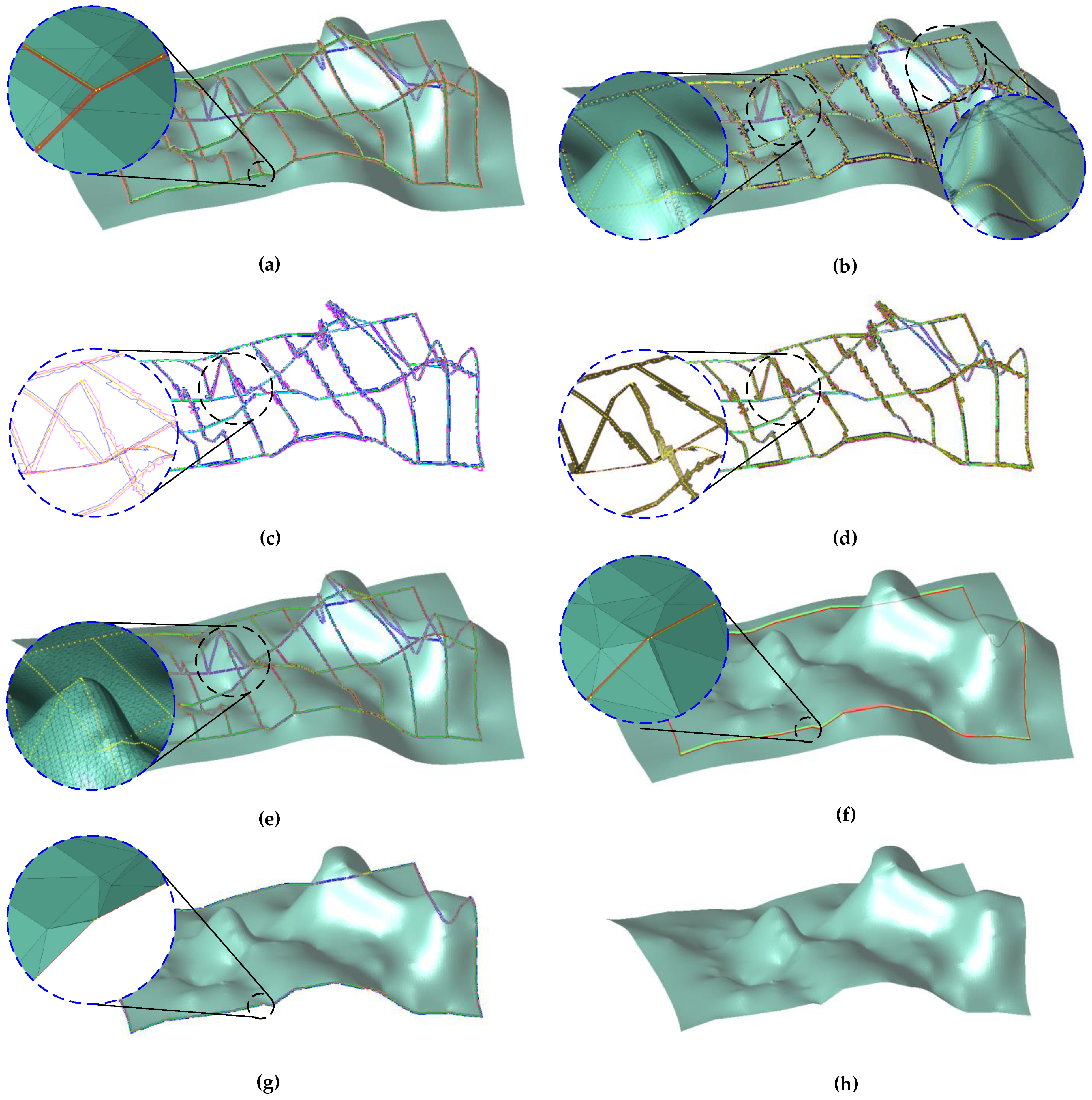
Based on the above idea regarding the snapping of the boundary constraint polylines, the steps involved in snapping non-boundary constraint polylines are as follows. As shown in Figure 6, firstly, the non-boundary constraint polyline ${\mathit{L}}_{n,i}$ should be projected onto the model $\mathit{M}$ generated based on implicit modeling, and a similar path with the same number of vertices as the non-boundary constraint polyline ${\mathit{L}}_{n,i}$ is obtained, which is defined as the non-boundary projective polyline ${\mathit{L}}_{n,i}^{\prime }\left\{i=1,2,\dots ,n\right\}$. Secondly, based on the location of the projective points on the non-boundary projective polyline ${\mathit{L}}_{n,i}^{\prime }$, the set of topologically continuous triangular patches ${\mathit{T}}_i\left\{i=1,2,\dots ,n\right\}$ on the path of the non-boundary projective polyline ${\mathit{L}}_{n,i}^{\prime }$ is searched, and the region formed by the set of triangular patches ${\mathit{T}}_i$ is defined as the projective neighborhood ${\mathit{R}}_i\left\{i=1,2,\dots ,n\right\}$ of the non-boundary constraint polyline ${\mathit{L}}_{n,i}$. Then, the contour polylines of the projective neighborhood ${\mathit{R}}_i$ on both sides of the non-boundary projective polyline ${\mathit{L}}_{n,i}^{\prime }$ are extracted as ${\mathit{L}}_{p,i,f}$ and ${\mathit{L}}_{p,i,s}$, and the set of triangular patches ${\mathit{T}}_i$ is deleted. Next, taking the constraint point on the non-boundary constraint polyline ${\mathit{L}}_{n,i}$ as the mesh vertex, the projective neighborhood ${\mathit{R}}_i$ is triangulated between ${\mathit{L}}_{n,i}$, ${\mathit{L}}_{p,i,f}$, and ${\mathit{L}}_{p,i,s}$, respectively, using the re-meshing method between two polylines to generate a new set of triangular patches ${\mathit{T}}_i^{\prime }\left\{i=1,2,\dots ,n\right\}$. Finally, the new model ${\mathit{M}}^{\prime }$ is generated by merging the re-meshing triangular patches ${\mathit{T}}_i^{\prime }$ in the projective neighborhood ${\mathit{R}}_i$ with the other patches of the model $\mathit{M}$, and the normal direction of all triangular patches is unified, which can achieve the accurate snapping of the orebody model with the non-boundary constraint polyline.

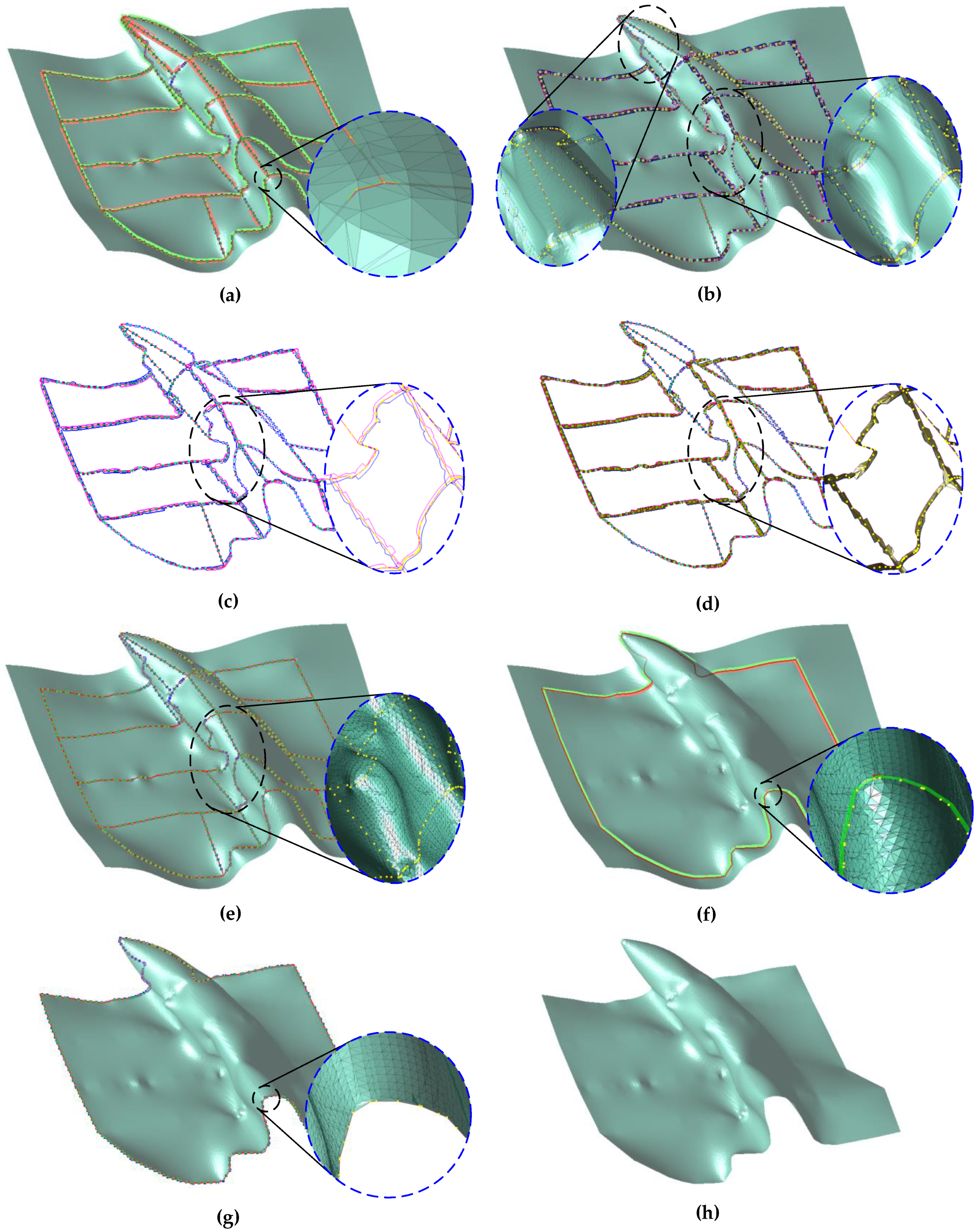
The snapping process of the boundary constraint polyline can be considered a special case of snapping of the non-boundary constraint polyline. As shown in Figure 7, compared with the non-boundary constraint polyline, only the contour polyline inside the projective neighborhood ${\mathsf{\Omega }}_i\left\{i=1,2,\dots ,n\right\}$ participates in re-meshing when the projective neighborhood ${\mathsf{\Omega }}_i$ of the boundary constraint polylines ${\mathit{L}}_{b,i}$ is re-meshed.

3.5. Boundary Clipping

The orebody has a specific shape and volume. To limit the scope of the model, it is necessary to construct the maximum bounding box in the coordinate system during the modeling process. Generally, the maximum bounding box is a 3D space with external geometric constraints. If the shape of the orebody model is equiaxed or columnar, the model can usually meet the modeling requirements when the maximum bounding box is larger than the model boundary. The model generated by means of the implicit modeling method is a spatially continuous closed entity. If the orebody model is platelike (such as a layer-type or vein-type model), taking a layer-type orebody as an example, the upper and lower models usually need to be built separately and then merged.

In fact, one can accurately control the upper and lower layers of the model within the boundary using the explicit modeling method to model the sub-meshes separately, but this depends greatly on human–computer interactions. The orebody model constructed using the implicit modeling method is essentially obtained via spatial interpolation. The spatial constraint data set determines the spatial morphology of the model. When the boundary range is controlled only by the maximum bounding box of the model, the size of the generated model usually does not conform to the actual boundary size of the model. Because the boundary of the orebody model is very irregular, it is very difficult to accurately construct the constraint of the maximum bounding box at the boundary.

It is worth noting that if the boundary of the orebody model can be determined in advance, the boundary range can be controlled in the implicit modeling process by defining boundary constraint polylines to provide one-way tangential constraints for the model, as shown in Figure 7a. If the boundary polyline of the orebody model is determined only after the model is generated, the part outside the model boundary can be clipped through post-processing. In this paper, a method of model boundary clipping is proposed to solve the problem of boundary mismatch in some orebody models.

To ensure the clipping effect, it is necessary to satisfy the following conditions before clipping boundaries. On the one hand, the boundary polyline should be closed, and the direction of the boundary polyline should be consistent with the direction of the boundary constraint polyline. On the other hand, the model should snap accurately to the constraint polylines. The steps involved in clipping boundaries are as follows, as shown in Figure 8 and Figure 9. First, a seed point is selected on the boundary polyline $\mathit{l}$. According to the sequence of points on the boundary polyline, the triangle edge formed by the seed point and its next point is defined as the initial edge ${\mathit{l}}_{i=1}\left\{i=1,2,\dots ,n\right\}$. Each triangle edge forming the boundary polyline is defined as the boundary triangle edge ${\mathit{l}}_i$. In addition, the direction of the boundary polyline can be directly judged according to the reserved side of the red tangential strip. Second, along the vector direction of the boundary polyline $\mathit{l}$, the whole boundary polyline is traversed from the initial edge. One can calculate the vector product of the direction vector and the normal vector of the boundary triangle edge ${\mathit{l}}_i$ to obtain the normal vector of the normal plane where the boundary triangle edge ${\mathit{l}}_i$ is located, as shown in Equation (6).

$${\mathit{n}}_{p,i}={\mathit{l}}_i^{\prime }\times {\mathit{n}}_i$$

(6)

where ${\mathit{l}}_i^{\prime }\left\{i=1,2,\dots ,n\right\}$ is the direction vector of the boundary triangle edge ${\mathit{l}}_i$, ${\mathit{n}}_i\left\{i=1,2,\dots ,n\right\}$ is the normal vector of the boundary triangle edge ${\mathit{l}}_i$, and ${\mathit{n}}_{p,i}\left\{i=1,2,\dots ,n\right\}$ is the normal vector of the normal plane where the boundary triangle edge ${\mathit{l}}_i$ is located, pointing to the inside of the model boundary.

Then, the normal vector ${\mathit{n}}_{p,i}=\left({\mathit{a}}_i, {\mathit{b}}_i,{\mathit{c}}_i\right)$ and a point ${\mathit{p}}_i=\left(x_i,y_i,z_i\right)$ on the triangle edge ${\mathit{l}}_i$ are substituted into the point-normal form equation of a plane to obtain the plane Equation (7) of the normal plane $\mathit{\alpha }$ where ${\mathit{l}}_i$ is located.

$$f_p\left(\mathit{x}\right)=a_i\left(x-x_i\right)+b_i\left(y-y_i\right)+c_i\left(z-z_i\right)$$

(7)

For the triangular mesh of the topological manifold, a triangle edge ${\mathit{l}}_i$ has two adjacent triangular patches, denoted as $t_{lef}$ and $t_{rig}$. To facilitate the processing of triangular patches, we add a label for each triangular patch, marked as $t_{lab}$. $t_{lab}=1$ indicates that the triangular patch will be retained and $t_{lab}=0$ indicates that the triangular patch will be deleted. Then, the vertex coordinates of the triangular patches $t_{lef}$ and $t_{rig}$ are substituted into Equation (7). If the function values $f_p\left(\mathit{x}\right)$ of all three vertices of the triangular patch $t_{lef}$ or $t_{rig}$ are greater than or equal to 0, then the label value of the triangular patch is set to 1 (i.e., $t_{lab}=1$). Otherwise, we set the label value of the triangular patch to 0 (i.e., $t_{lab}=0$). Then, we set the unlabeled triangular patches adjacent to it to the same label. Next, based on the existing labels, the breadth-first search algorithm (i.e., BFS) is used to traverse all unlabeled triangular patches. We set the label value of the unlabeled triangular patch adjacent to the triangular patch with $t_{lab}=1$ or $t_{lab}=0$ to 1 or 0, respectively. Finally, we delete all triangular patches with $t_{lab}=0$ to clip the boundary of the orebody model. In addition, the orebody model may have more than one boundary. The above method can be applied to clip multiple boundaries simultaneously.

4. Results

4.1. Examples

Based on the above method, the feature snapping and boundary clipping processes of the model were realized using Microsoft Visual Studio 2013 (C++ language) (Microsoft, Redmond, WA, USA) and were tested on some real geological data sets, which resulted in the accurate snapping of the feature data of the orebody model and the accurate clipping of the model boundary, as shown in Figure 10, Figure 11, Figure 12, Figure 13 and Figure 14. The experimental results showed that the method and algorithm proposed in this paper are automatic and practical in improving the precision of an orebody model.

To test the snapping effect of feature points, we selected a portion of the borehole data, and the borehole samples were combined into internal constraint polylines and external constraint polylines according to the ore grade, as shown in Figure 10a. The orebody model obtained through implicit modeling should include the internal constraint polylines inside the model and leave the external constraint polylines outside the model. In Figure 10b, it can be seen that some internal constraint polylines of some boreholes were left exposed outside the model in the implicit modeling results. According to the requirement of the 3D refinement modeling of the orebody, the orebody model should accurately snap to contact points of internal and external constraint polylines of the orebody. To achieve the goal of accurately snapping the model to the contact points, the constraint points were added at the position of the contact points that were not snapped, as shown in Figure 10c. Finally, the orebody model was snapped to the contact points of the internal and external constraint polylines using the above method of snapping constraint points, as shown in Figure 10d. The experiments showed that this method can achieve the desired effect in the process of snapping the orebody model to the given constraint points (i.e., the feature points). In addition, after calculation, the volume of the ore body model after the snapping of the features increased by about 65,441 cubic meters, which has great economic value for mining enterprises.

To fully test the effect of the orebody model with snapping of the feature polylines, we selected four groups of data with different levels of complexity, as shown in Figure 11, Figure 12, Figure 13 and Figure 14. It is worth noting that since geologic bodies are generally large in scale, we only used a part of the orebody for testing. The first group of data was relatively simple so that the test process could be shown more intuitively and clearly, as shown in Figure 11. The orebody model was generated via implicit modeling based on the constraint polylines converted using the feature polylines, taking the non-boundary constraint polylines as an example, as shown in Figure 11a. It can be seen that there were non-negligible gaps between the generated model and the constraint polylines, and thus this cannot meet the requirements of refinement modeling.

To snap the model to all features, the constraint polylines were first projected to the model surface to obtain the projective polylines of the constraint polylines. Based on the projection points on the projective polylines, we searched and determined the topologically continuous projective neighborhood, as shown in Figure 11b. Second, we extracted the contour polylines of the projective neighborhood on both sides of the projective polyline, and deleted the matched triangular mesh in the projective neighborhood, as shown in Figure 11c. Then, the projective neighborhood was re-meshed with the constraint polyline as the center polyline, as shown in Figure 11d. Finally, the snapping of constraint polylines was realized by merging all triangular patches on the model surface and unifying the normal direction of triangular patches, as shown in Figure 11e. It can be seen that the mesh topology of the orebody model was completely consistent with the feature polylines after the constraint polylines were snapped, eliminating the original gaps between the model and the feature polylines, thus achieving a satisfying effect.

Furthermore, to ensure that the contour of the orebody model was consistent with the actual boundary, the boundary polyline and the snapped model were retained, as shown in Figure 11f. Then, the model boundary was clipped according to the boundary clipping method. It can be seen that the model after boundary clipping was still topologically consistent with the boundary feature polyline, meeting the requirements of 3D refinement modeling of the orebody, as shown in Figure 11g. The final orebody model obtained after mesh processing is shown in Figure 11h.

As shown in Figure 12, Figure 13 and Figure 14, we used three groups of complex orebody model data for testing. The test results showed that the method in this paper was able to better solve the problem of the inaccurate snapping of model constraint polylines (or feature polylines) after implicit modeling. In summary, the results show that our methods are conducive to the accurate snapping of the orebody model with feature points and feature polylines, and the accurate control of the orebody model boundary.

The test results above show that the geometry topology of the model boundary and the boundary constraint polyline were consistent after clipping, which is beneficial to mesh stitching modeling. On the one hand, for each mesh of the orebody model, the required model could be generated by using the mesh splicing method after implicit modeling, model snapping, and boundary clipping, respectively. On the other hand, for the layered orebody model, the upper and lower models of the orebody could be constructed respectively, so that the two-layer models could be spliced to construct the orebody model. To show the modeling effect of mesh splicing, we selected a layered orebody model for demonstration, as shown in Figure 15. In Figure 15b, it can be seen that the splicing effect of mesh boundaries in each mesh of the lower model of the orebody was good, and the mesh points at mesh boundaries corresponded to the mesh edges one by one. In addition, when the upper and lower models of the orebody were constructed and spliced, respectively, the mesh topology of the boundary contact positions of the upper and lower models was also good, as shown in Figure 15e. Therefore, our method of clipping the model boundary is feasible and effective.

4.2. Performance

In this paper, the main factors affecting the performance of model snapping and boundary clipping included the geometric complexity of the original model and the feature number to be snapped. We implemented the algorithm in C++ and tested it on a Windows 64-bit computer (Microsoft, Redmond, WA, USA) with a 3.80 GHz Intel (R) Core (TM) i7-10700 K processor, 64 GB RAM, and NVIDIA GeForce RTX 2060 GPU.

Table 1. Experimental data statistics, including the constraint polyline number ($N_l$), the constraint point number ($N_p$), the model unit size ($S_u$), the triangular patch number of the original model ($N_t$), the change in the number of triangular patches before and after snapping the model’s features ($\Delta N_{t,s}$), the change in the number of triangular patches before and after clipping the model’s boundary ($\Delta N_{t,c}$), the model snapping ratio ($R_{sna}$), the model snapping time ($T_{sna}$), and the boundary clipping time ($T_{c\mathit{L}i}$).

Examples	${\mathit{N}}_{\mathit{l}}/\mathit{n}$	${\mathit{N}}_{\mathit{p}}/\mathit{n}$	${\mathit{S}}_{\mathit{u}}/\mathit{m}$	${\mathit{N}}_{\mathit{t}}/\mathit{n}$	$\Delta {\mathit{N}}_{\mathit{t},\mathit{s}}/\mathit{n}$	$\Delta {\mathit{N}}_{\mathit{t},\mathit{c}}/\mathit{n}$	${\mathit{R}}_{\mathit{s}\mathit{n}\mathit{a}}/\%$	${\mathit{T}}_{\mathit{s}\mathit{n}\mathit{a}}/\mathit{s}$	${\mathit{T}}_{\mathit{c}\mathit{l}\mathit{i}}/\mathit{s}$
Figure 10	65	132	2.4	117,580	+388	---	100	0.27	---
Figure 11	9	950	0.5	15,157	+119	−9581	100	0.62	0.54
Figure 12	48	3792	1	48,089	+2293	−14,508	100	5.25	1.14
Figure 13	74	6529	1	80,428	+3926	−22,423	97.30	13.20	2.58
Figure 14	48	2104	1	81,516	+1750	−25,899	91.67	17.22	3.34

shows the statistics obtained using our method in these examples. In Table 1, it can be seen, as also shown in Figure 10, Figure 11, Figure 12, Figure 13 and Figure 14, that the number of triangular patches of the orebody model increased significantly after the model was snapped. This was the result of re-meshing the mesh matched by the constraint data when snapping the model. In addition, the number of triangular patches of the model was significantly reduced after the model boundary was clipped. As can be seen in Figure 11, Figure 12 and Figure 13, the model’s snapping time and boundary clipping time tended to increase with the increase in the number of constraint data to be snapped. As can be seen in Figure 13 and Figure 14, as the model geometry became more complex, some constraint data were not easily snapped, and the processes of model snapping and boundary clipping required a longer computing time. However, in general, our method and algorithm performed well in terms of the model snapping ratio, the model snapping time, and the boundary clipping time, and the effect on orebody modeling applications also met the actual needs of practical applications.

4.3. Discussion

This snapping method employed in this model is suitable for cases in which the feature points and feature polylines are close to the mesh model and the shape trend does not change much. If the mesh model obtained via implicit modeling conforms to the corresponding constraint points (feature points) and constraint polylines (feature polylines) within a given modeling accuracy, this method can satisfy the needs of practical applications in mines. However, the local dynamic updating method of orebody models based on mesh reconstruction and mesh deformation proposed by Li et al. [44] is suitable for cases in which the updated interpretation polyline is a certain distance from the ore body model. For the application of orebody modeling, the main factors affecting the performance of the algorithm include the following three aspects: the reliability of matching the nearest point, the reliability of the matching mesh, and the quality of the re-meshing of the matching mesh. The closest point of the match provides the basis for searching the matching mesh. The matched mesh determines the area of feature points or feature polylines to re-mesh. Incorrect matching of the closest points or meshes can lead to errors such as warping of the snapped meshes. The re-meshing process of the matching mesh is the key to the model snapping method. Considering that there is no reliable method for polygonal triangulation at present, it is necessary to further improve the method or study more reliable model snapping methods in the future. Among these, a feasible idea is to consider the prior rules of the existing meshes in the process of polygon triangulation.

5. Conclusions

In this paper, we have proposed a method to accurately snap the model feature points and feature polylines after implicit orebody modeling. This method is suitable for cases in which the feature points and feature polylines are close to the orebody mesh model and the shape trend changes little. Due to the ambiguity and lack of features in the processes of implicit surface interpolation and implicit surface reconstruction, it is difficult for the model to accurately snap the features of the orebody in the modeling of a complex orebody. The innovation of this paper is that the proposed method can snap the features of the orebody mesh model obtained by means of any iso-surface extraction method, and thus it has wider applicability. We have solved the feature loss problem of orebody models obtained via implicit modeling through a mesh processing method, which greatly improves the accuracy and reliability of the orebody geometric model. In addition, we have also proposed a boundary clipping method for the orebody model, which is suitable for accurate boundary clipping of the model after feature snapping. Through experimental tests conducted with a large number of real orebody modeling data, the results showed that the method proposed in this paper could not only snap model feature data accurately but also required a small amount of calculation and displayed high efficiency.

References

1. Gong, J.; Cheng, P.; Wang, Y. Three-dimensional modeling and application in geological exploration engineering. Comput. Geosci. 2004, 30, 391–404. [Google Scholar] [CrossRef]
2. Whitten, E.H.T. Mathematical geology in perspective: Has objective hypothesis testing become overlooked? Math. Geol. 2003, 35, 1–8. [Google Scholar] [CrossRef]
3. Jin, B.-X.; Fang, Y.-M.; Song, W.-W. 3D visualization model and key techniques for digital mine. Trans. Nonferrous Met. Soc. China 2011, 21, s748–s752. [Google Scholar] [CrossRef]
4. Uronen, P.; Matikainen, R. The Intelligent Mine. IFAC Proc. Vol. 1995, 28, 9–19. [Google Scholar] [CrossRef]
5. Mao, X.; Zhang, B.; Deng, H.; Zou, Y.; Chen, J. Three-dimensional morphological analysis method for geologic bodies and its parallel implementation. Comput. Geosci. 2016, 96, 11–22. [Google Scholar] [CrossRef]
6. Bardzinski, P.; Jurdziak, L.; Kawalec, W.; Król, R. Copper Ore Quality Tracking in a Belt Conveyor System Using Simulation Tools. Nonrenewable Resour. 2019, 29, 1031–1040. [Google Scholar] [CrossRef] [Green Version]
7. Li, Y.L.; Gao, J.G. Research and Application of the 3D Mathematic Model of Ore-Body Based on Suppac Software—Yunnan White Cattle Factory Silver Polymetallic Mine. Adv. Mater. Res. 2013, 868, 84–87. [Google Scholar] [CrossRef]
8. Yun, B.; Pengfei, Z.; Jing, Z.; Weihao, K.; Xiaocui, L.; Ke, C.; Lu, S.; Linying, L. Application of geo-statistics in calculation of a uranium deposit. E3S Web Conf. 2020, 206, 01005. [Google Scholar] [CrossRef]
9. Zhiwei, H.; Jun, S.; Kaibin, H.; Yalin, L. Mining 3D Visualization Simulation and Safety Evaluation. In Proceedings of the 2011 Fifth International Conference on Management of e-Commerce and e-Government, Wuhan, China, 5–6 November 2011; pp. 261–268. [Google Scholar]
10. Liu, X.; Qiang, Z.; Wang, H.; Fei, S.; Cui, Y.; Wang, J.; Zhang, Z.; You, L. Application of High Precision 3D Geological Modeling in Horizontal Well Development of Tight Gas Reservoir. In Proceedings of the 2020 2nd International Conference on Artificial Intelligence and Advanced Manufacture (AIAM), Manchester, UK, 15–17 October 2020; pp. 325–329. [Google Scholar] [CrossRef]
11. Tang, B.Y.; Wu, C.L.; Li, X.C. A fine 3D geological modeling method based on TIN-CPG hybrid spatial data model. Rock Soil Mech. 2017, 38, 1218–1225. [Google Scholar]
12. Birch, C. New systems for geological modelling—black box or best practice? J. Southern Afr. Inst. Mining Metallurgy 2014, 114, 993–1000. [Google Scholar]
13. Cowan, E.J.; Beatson, R.K.; Ross, H.J.; Fright, W.R.; McLennan, T.J.; Evans, T.R.; Carr, J.C.; Lane, R.G.; Bright, D.V.; Gillman, A.J.; et al. In Practical implicit geological modelling. In Proceedings of the 5th International Mining Geology Conference, Bendigo, Australia, 17–19 November 2003; Australasian Inst Mining & Metallurgy: Bendigo, Australia, 2003; pp. 89–99. [Google Scholar]
14. Guo, J.; Wang, J.; Wu, L.; Liu, C.; Li, C.; Li, F.; Lin, M.; Jessell, M.W.; Li, P.; Dai, X.; et al. Explicit-implicit-integrated 3-D geological modelling approach: A case study of the Xianyan Demolition Volcano (Fujian, China). Tectonophysics 2020, 795, 228648. [Google Scholar] [CrossRef]
15. Wang, J.; Zhao, H.; Bi, L.; Wang, L. Implicit 3D Modeling of Ore Body from Geological Boreholes Data Using Hermite Radial Basis Functions. Minerals 2018, 8, 443. [Google Scholar] [CrossRef] [Green Version]
16. Zhong, D.; Wang, L. Solution Optimization of RBF Interpolation for Implicit Modeling of Orebody. IEEE Access 2020, 8, 13781–13791. [Google Scholar] [CrossRef]
17. Zhong, D.-Y.; Wang, L.; Bi, L. Implicit surface reconstruction based on generalized radial basis functions interpolant with distinct constraints. Appl. Math. Model. 2019, 71, 408–420. [Google Scholar] [CrossRef]
18. Zhong, D.; Wang, L.; Bi, L. Extended Hermite Radial Basis Functions for Sparse Contours Interpolation. IEEE Access 2020, 8, 58752–58762. [Google Scholar] [CrossRef]
19. Zhong, D.-Y.; Wang, L.-G.; Bi, L.; Jia, M.-T. Implicit modeling of complex orebody with constraints of geological rules. Trans. Nonferrous Met. Soc. China 2019, 29, 2392–2399. [Google Scholar] [CrossRef]
20. Yamamoto, J.K.; Koike, K.; Kikuda, A.T.; Campanha, G.A.D.C.; Endlen, A. Post-processing for uncertainty reduction in computed 3D geological models. Tectonophysics 2014, 633, 232–245. [Google Scholar] [CrossRef]
21. Saptawati, G.A.P.; Nata, G.N.M. Knowledge discovery on drilling data to predict potential gold deposit. In Proceedings of the 2015 International Conference on Data and Software Engineering, Yogyakarta, Indonesia, 25–26 November 2015; pp. 143–147. [Google Scholar] [CrossRef]
22. Peng, J.; Hu, J.; Dai, H. Automatic Modeling Algorithm Research and Application of Complex Structural Geology in Three-Dimensional Space. In Proceedings of the 6th International Conference on Wireless Communications, Networking and Mobile Computing (WICOM), Chengdu, China, 23–25 September 2010; pp. 1–4. [Google Scholar] [CrossRef]
23. Wang, J.; Zhang, J. 3D Fine Geological Modeling of the High Water Cut Stage Reservoir: A Case Study of the ES2S1 Reservoir in the Southern Pucheng Oilfield. In Proceedings of the 2010 Second International Conference on Modeling, Simulation and Visualization Methods, Sanya, China, 15–16 May 2010; pp. 106–109. [Google Scholar] [CrossRef]
24. Macêdo, I.; Gois, J.P.; Velho, L. Hermite Interpolation of Implicit Surfaces with Radial Basis Functions. In Proceedings of the 22nd Brazilian Symposium on Computer Graphics and Image Processing, Rio de Janeiro, Brazil, 11–15 October 2009; pp. 1–8. [Google Scholar] [CrossRef] [Green Version]
25. Zhong, D.; Zhang, J.; Wang, L. Fast Implicit Surface Reconstruction for the Radial Basis Functions Interpolant. Appl. Sci. 2019, 9, 5335. [Google Scholar] [CrossRef] [Green Version]
26. Custodio, L.; Etiene, T.; Pesco, S.; Silva, C. Practical considerations on Marching Cubes 33 topological correctness. Comput. Graph. 2013, 37, 840–850. [Google Scholar] [CrossRef] [Green Version]
27. Yu, R.H.; Xie, W.; Wu, L.D.; Hao, H.X. In Research on Multi—resolution Isosurface Extraction Method for 3D Scalar Field. In Proceedings of the 2nd IEEE International Conference on Data Science in Cyberspace (DSC), Shenzhen, China, 26–29 June 2017; pp. 359–362. [Google Scholar]
28. Montani, C.; Scateni, R.; Scopigno, R. A modified look-up table for implicit disambiguation of Marching Cubes. Vis. Comput. 1994, 10, 353–355. [Google Scholar] [CrossRef]
29. Nielson, G.; Hamann, B. The asymptotic decider: Resolving the ambiguity in marching cubes. In Proceedings of the Proceeding Visualization ‘91, San Diego, CA, USA, 22–25 October 1991; pp. 83–91. [Google Scholar] [CrossRef]
30. Feng, S.W.; Zhang, J.; Zeng, B. In Study of Feature Reconstruction Algorithm for Surface Mesh. In Proceedings of the IEEE International Conference on Robotics and Biomimetics (ROBIO), Guilin, China, 19–23 December 2009; pp. 2157–2162. [Google Scholar]
31. Wang, J.; Gu, D.; Gao, Z.; Yu, Z.; Tan, C.; Zhou, L. Feature-Based Solid Model Reconstruction. J. Comput. Inf. Sci. Eng. 2013, 13, 011004. [Google Scholar] [CrossRef]
32. Zhao, X.; Zhou, Z.; Duan, Y.; Wu, W. Detail-feature-preserving surface reconstruction. Comput. Animat. Virtual Worlds 2012, 23, 407–416. [Google Scholar] [CrossRef]
33. Xi, Y.; Duan, Y. A novel region-growing based iso-surface extraction algorithm. Comput. Graph. 2008, 32, 647–654. [Google Scholar] [CrossRef]
34. Cebral, J.R.; Camelli, F.E.; Löhner, R. A feature-preserving volumetric technique to merge surface triangulations. Int. J. Numer. Methods Eng. 2002, 55, 177–190. [Google Scholar] [CrossRef]
35. Subedi, S.C.; Verma, C.S.; Suresh, K. A Review of Methods for the Geometric Post-Processing of Topology Optimized Models. J. Comput. Inf. Sci. Eng. 2020, 20, 060801. [Google Scholar] [CrossRef]
36. Jakob, W.; Tarini, M.; Panozzo, D.; Sorkine-Hornung, O. Instant field-aligned meshes. ACM Trans. Graph. 2015, 34, 1–15. [Google Scholar] [CrossRef]
37. Zhan, Q.; Chen, X. Boolean Combinations of Implicit Functions for Model Clipping in Computer-Assisted Surgical Planning. PLoS ONE 2016, 11, e0145987. [Google Scholar] [CrossRef] [Green Version]
38. Nguyen, Q.T.; Gomes, A.J. Healed marching cubes algorithm for non-manifold implicit surfaces. In Proceedings of the 23rd Portuguese Meeting on Computer Graphics and Interaction (EPCGI), Covilha, Portugal, 24–25 November 2016; pp. 1–8. [Google Scholar] [CrossRef]
39. Carr, J.C.; Beatson, R.K.; Cherrie, J.B.; Mitchell, T.J.; Fright, W.R.; McCallum, B.C.; Evans, T.R. Reconstruction and Representation of 3D Objects with Radial Basis Functions. In Proceedings of the 28th Annual Conference on Computer Graphics and Interactive Techniques, Los Angeles, CA, USA, 12–17 August 2001; pp. 67–76. [Google Scholar]
40. Beatson, R.K.; Light, W.A.; Billings, S. Fast Solution of the Radial Basis Function Interpolation Equations: Domain Decomposition Methods. SIAM J. Sci. Comput. 2001, 22, 1717–1740. [Google Scholar] [CrossRef] [Green Version]
41. Christiansen, H.N.; Sederberg, T.W. Conversion of complex contour line definitions into polygonal element mosaics. ACM Siggraph Comput. Graph. 1978, 12, 187–192. [Google Scholar] [CrossRef]
42. Fuchs, H.; Kedem, Z.M.; Uselton, S.P. Optimal surface reconstruction from planar contours. Commun. ACM 1977, 20, 693–702. [Google Scholar] [CrossRef]
43. Ganapathy, S.; Dennehy, T.G. A new general triangulation method for planar contours. ACM Siggraph Comput. Graph. 1982, 16, 69–75. [Google Scholar] [CrossRef]
44. Li, Z.; Zhong, D.; Wu, Z.; Wang, L.; Tang, Q. Local Dynamic Updating Method of Orebody Model Based on Mesh Reconstruction and Mesh Deformation. Minerals 2021, 11, 1232. [Google Scholar] [CrossRef]
Figure 1. Reasons for inaccurate snapping in implicit surface reconstruction. (a,b) show the two different surface reconstruction results caused by ambiguity in the vertex state of the same voxel unit. (c,d) show the phenomenon of the loss of features after surface reconstruction due to the defects of the iso-surface extraction algorithm. (e) shows an example of implicit surface reconstruction of an orebody based on borehole constraints.
Mathematics 10 02593 g001
Figure 2. Overall flow chart of a mesh processing method, with snapping of the features of an orebody model.
Mathematics 10 02593 g002
Figure 3. Constraint data for implicit modeling. (a) shows the constraint points. (b) shows the non-boundary constraint polyline. (c) shows the boundary constraint polyline.
Mathematics 10 02593 g003
Figure 4. Snap constraint points. (a) shows the mesh before snapping of the constraint points. (b) shows the mesh after snapping of the constraint points. (c) shows the influence of snapping constraint points on the mesh model.
Mathematics 10 02593 g004
Figure 5. Remeshing between polylines. (a) shows the initial polylines. (b) shows the initial matched point. (c) shows the results of the preprocessing of polylines and alignment of the point column direction. (d) shows the results of matching the vertices of the first set of polylines based on the triangulation rules. (e) shows the results of matching the vertices of the second set of polylines based on the triangulation rules. (f) shows the solid model after re-meshing.
Mathematics 10 02593 g005
Figure 6. Snapping of non-boundary constraint polylines. (a) shows the non-boundary constraint polylines. (b) shows the process of projecting constraint polylines onto the model and matching the meshes. (c) shows the results of deleting the matched meshes and extracting the boundaries of the projective neighborhoods. (d) shows the result of re-meshing the projective neighborhoods. (e) shows the results of merging all meshes and unifying the normal direction of all triangular patches. (f) shows the mesh model after snapping constraint polylines. ① shows the implicit modeling result. ② shows the matched meshes to be deleted.
Mathematics 10 02593 g006
Figure 7. Snapping of boundary constraint polylines. (a) shows the boundary constraint polylines and non-boundary constraint polylines. (b) shows the process of projecting constraint polylines onto the model and matching the meshes. (c) shows the results of deleting the matched meshes and extracting the boundaries of the projective neighborhoods. (d) shows the result of re-meshing the projective neighborhoods. (e) shows the results of merging all meshes and unifying the normal direction of all triangular patches. (f) shows the mesh model after snapping constraint polylines. ① shows the implicit modeling result. ② shows the matched meshes to be deleted.
Mathematics 10 02593 g007
Figure 8. Judgment and marking method for the inside and outside triangular patches of the model boundary. (a) shows the judgment method of the inside and outside triangular patches of the model boundary, the blue patch is on the inside of the boundary, and the green patch is on the outside of the boundary. (b) shows the marking method for the inside and outside triangular patches of the model boundary.
Mathematics 10 02593 g008
Figure 9. Mesh boundary clipping process. (a) shows the selection of seed points and initial edges on the boundary polyline and the marking of triangular patches adjacent to the initial edges. (b) shows the result of marking the triangular patches adjacent to the whole boundary polyline. (c) shows the result of marking all triangular patches based on the marked triangular patches. (d) shows the result of deleting all triangular patches with a label value of 0.
Mathematics 10 02593 g009
Figure 10. The test result of the snapping of feature points. (a) shows the borehole constraints. (b) shows the implicit modeling results of the ore body. (c) shows the orebody model before the snapping of feature points. (d) shows the orebody model after the snapping of feature points.
Mathematics 10 02593 g010
Figure 11. The first group test results of the snapping of feature polylines and clipping of the model boundary. (a) shows constraint polylines and implicit modeling results. (b) shows the process of constraint polyline projection and mesh matching. (c) shows the matched mesh boundaries. (d) shows the re-meshing of the matching meshes. (e) shows the results of mesh merging and normal consistency. (f) shows the boundary constraint polylines and the model after normal consistency. (g) shows the result of mesh boundary clipping. (h) shows the orebody model after mesh processing.
Mathematics 10 02593 g011
Figure 12. The second group test results of the snapping of feature polylines and the clipping of the model boundary. (a) shows constraint polylines and implicit modeling results. (b) shows the process of constraint polyline projection and mesh matching. (c) shows the matched mesh boundaries. (d) shows the re-meshing of the matching meshes. (e) shows the results of mesh merging and normal consistency. (f) shows the boundary constraint polylines and the model after normal consistency. (g) shows the result of mesh boundary clipping. (h) shows the orebody model after mesh processing.
Mathematics 10 02593 g012
Figure 13. The third group test results of the snapping of feature polylines and the clipping of the model boundary. (a) shows constraint polylines and implicit modeling results. (b) shows the process of constraint polyline projection and mesh matching. (c) shows the matched mesh boundaries. (d) shows the re-meshing of the matching meshes. (e) shows the results of mesh merging and normal consistency. (f) shows the boundary constraint polylines and the model after normal consistency. (g) shows the result of mesh boundary clipping. (h) shows the orebody model after mesh processing.
Mathematics 10 02593 g013
Figure 14. The fourth group test results of the snapping of feature polylines and the clipping of the model boundary. (a) shows constraint polylines and implicit modeling results. (b) shows the process of constraint polyline projection and mesh matching. (c) shows the matched mesh boundaries. (d) shows the re-meshing of the matching meshes. (e) shows the results of mesh merging and normal consistency. (f) shows the boundary constraint polylines and the model after normal consistency. (g) shows the result of mesh boundary clipping. (h) shows the orebody model after mesh processing.
Mathematics 10 02593 g014
Figure 15. The splicing effect of a layered orebody model based on model clipping. (a) shows the mesh boundary polyline of each mesh in the lower layer of the layered orebody model. (b) shows the effect of orebody modeling and boundary clipping of each mesh. (c) shows the result of merging all meshes of the lower layer. (d) shows the upper mesh of the layered orebody model. (e) shows the splicing effect of upper and lower meshes. (f) shows the final layered orebody model. The labels ① to ⑥ show the individual sub-meshes for modeling.
Mathematics 10 02593 g015