Article

Some Important Points of the Josephson Effect via Two Superconductors in Complex Bases

by
Fernando S. Vidal Causanilles
1,
Haci Mehmet Baskonus
2,
Juan Luis García Guirao
1,3,* and
Germán Rodríguez Bermúdez
4
1
Departamento de Matemática Aplicada y Estadística, Universidad Politécnica de Cartagena, Hospital de Marina, 30203 Cartagena, Spain
2
Department of Mathematics and Science Education, Faculty of Education, Harran University, Sanliurfa 63510, Turkey
3
Department of Mathematics, Faculty of Science, King Abdulaziz University, P.O. Box 80203, Jeddah 21589, Saudi Arabia
4
University Centre of Defence at the Spanish Air Force Academy, UPCT-MDE Calle Coronel Lopez Pen a, s/n, Santiago de la Ribera, 30720 Murcia, Spain
*
Author to whom correspondence should be addressed.
Mathematics 2022, 10(15), 2591; https://doi.org/10.3390/math10152591
Submission received: 15 June 2022 / Revised: 20 July 2022 / Accepted: 22 July 2022 / Published: 25 July 2022
(This article belongs to the Special Issue Applications of Partial Differential Equations in Engineering)

Abstract

:
In this paper, we study the extraction of some analytical solutions to the nonlinear perturbed sine-Gordon equation with the long Josephson junction properties. The model studied was formed to observe the long Josephson junction properties separated by two superconductors. Moreover, it is also used to explain the Josephson effect arising in the highly nonlinear nature of the Josephson junctions. This provides the shunt inductances to realize a Josephson left-handed transmission line. A powerful scheme is used to extract the complex function solutions. These complex results are used to explain deeper properties of Josephson effects in the frame of impedance. Various simulations of solutions obtained in this paper are also reported.

1. Introduction

In 1962, the British physicist Brian David Josephson discovered a mathematical relation between current and voltage [1,2]. Via this relation, he explored an effect which produces a current, known as a supercurrent. This is called the Josephson effect (JE). Basically, this effect flows continuously without any voltage applied, across a device known as a Josephson junction (JJ) [3]. Moreover, this effect is also found through a tunnel based on the behavior of electrons. Then, the important properties of electrons between two superconductors were discovered. Later, Anderson and Rowell studied the Josephson tunnel’s effect on the electrons [4]. They remarked that the effect should be quite sensitive to magnetic fields, and also that the effect can only occur if both metals are superconducting and should be proportional to a special point. In 1966, Zharkov investigated the Josephson tunnel effect by using a wave function arising in the Ginzburg–Landau phenomenological theory of superconductivity, which also follows from a microscopic treatment of the problem [5]. The dynamics of a long linear Josephson tunnel junction with overlap geometry was numerically investigated in [6]. The current–voltage characteristics were observed in [7]. They studied the surface losses term and the external load matching [8]. In 2006, Ha and Nakagiri proposed a damped sine-Gordon equation given as [9]:
u t t + α u x x β u + γ = δ f .
Another type of this equation is given as [10,11,12]:
u t t u x x + sin ( u ) = ϵ ( γ α u t + β u x x t ) ,
where u = u ( x , t ) , ϵ 0 . In Equation (1), u ( x , t ) is used to define the phase difference of the electrons between the top and the bottom superconductor [13]. α u t (ohmic losses) and β u x x t terms (surface losses) are used to symbolize the energy losses. The meaning of parameters is shown in Table 1.
In Equation (1), if ϵ = 0 , it is completely converted an integrable model, and it also has a Hamiltonian structure. If γ = 0 and α = 0 ,
u t t u x x + sin ( u ) = ε u x x t ,
which is named the perturbed differential equation, and it is used to explain the current along a dielective barrier of the Josephson effect [9]. In 1987, Kivshar and Malomed investigated the inelastic interactions of kink properties [14,15]. They predicted the momentum and energy between the fast soliton and slow soliton. With the help of the fundamental optimal control theory, the existence of and necessary conditions for the optimal constant parameters were presented in [16]. The transposition method was used with the help of Hilbert theory and Interpolation and Variational theory [17]. Via tunnel Hamiltonian description, the Josephson current was theoretically studied in the properties of Green’s function [18]. Pagano presented the fabrication technology productions of the Josephson effect in terms of weak superconductivity used to explain the properties of two superconductors [19]. Seidel introduced various types of thin film Josephson in [20]. The current–voltage characteristics are given by the standard Resistively-Shunted-Junction circuit model in [21], and produced a high-Tc superconductor Josephson junction by way of the Helium Ion Beam technique, and studied their various properties in the 10 to 40 GHz range. In this paper, our aim is to extract more complex roots of Equation (1) in a complex basis under the rules of a powerful scheme. We will determine the strain conditions from these solutions and explain a Josephson effect in impedance between two superconductors. Moreover, we try to observe how the Josephson effect may be seen via simulations.
The rest of this paper is organized as follows: the mathematical analysis of the perturbed sine-Gordon Equation (PSGE) is given in Section 1. The theoretical analysis of the scheme proposed and applied is presented in Section 2. The method is implemented to find analytical solutions of the model in Section 3. The physical properties of the solutions obtained are reported in Section 4. Some important remarks and discussions are given in Section 5. In the last section of the paper, the conclusion is presented.

2. Theoretical Analysis of Scheme

In this section, a powerful scheme, namely, the Bernoulli sub-equation function method (BSEFM) is presented to find some results. It is summarized as follows [22,23,24].
Step 1. We consider the following nonlinear partial differential equation (NLPDE):
P ( u x , u t , u x t , u x x , ) = 0 ,
where u = u ( x , t ) . If we consider the transformation formula
u ( x , t ) = U ( η ) , η = k x c t , k 0 , c 0 ,
into Equation (2), we obtain the following nonlinear ordinary differential Equation (NODE),
N ( U , U , U , ) = 0 ,
in which U = U ( η ) , U = d U d η , U = d 2 U d η 2 , .
Step 2. According to general properties of BSEFM, the test function of solution of Equation (4) is considered as:
U ( η ) = i = 0 n a i F i = a 0 + a 1 F + a 2 F 2 + + a n F n ,
where F is defined as Bernoulli differential equation given by:
F = b F + d F M , b 0 , d 0 , M 0 , M 1 ,
where F = F ( η ) has the following two important solutions:
F ( η ) = d b + E e b ( M 1 ) η 1 1 M , b d F ( η ) = ( E 1 ) + ( E + 1 ) tanh b ( 1 M ) η 2 1 tanh b ( 1 M ) η 2 1 1 M , b = d .
b , d and a i will be determined later. Putting Equation (5) into Equation (4), we obtain an algebraic equation of F given as:
Ω ( F ) = ρ s F s + + ρ 1 F + ρ 0 = 0 .
Step 3. When we consider that the coefficients of Ω ( F ) equal zero, we find a system of algebraic equations of F given as:
ρ i = 0 , i = 0 , , s .
Solving this system, we find the values of a 0 , , a n which produce some analytical solutions to Equation (2).

3. Applications

In this part, we investigate the complex solutions of Equation (1) by using BSEFM. Considering the wave transformation defined by:
u ( x , t ) = U ( ξ ) , ξ = k x c t ,
where k 0 , c 0 for Equation (1), we convert it to the following NODE:
ϵ β c k 2 U + ( c 2 k 2 ) U α ϵ c U + U 1 6 U 3 ϵ γ = 0 .
According to the Balance principle, a relation between M and n is obtained as 3 M = 2 n + 3 . The following cases are derived from 3 M = 2 n + 3 .
Case-1 When M = 3 , n = 3 , it produces the first test function of solution formula as:
U ( ξ ) = a 0 + a 1 F + a 2 F 2 + a 3 F 3 ,
in which F = b F + d F 3 and also b 0 , d 0 . Putting Equation (12) into Equation (11), we extract the following cases:
Case-1.1a Under the term of b d , we obtain the following parameters values:
γ = 0 , c = i 3 7 4 b 2 k 2 2 b , a 3 = i 3 2 d 3 2 b 3 2 , α = 187 i 15 7 ϵ 3 28 b 2 k 2 , a 0 = 0 , a 1 = 3 i 3 2 d b , a 2 = 0 , β = i 30 7 b 2 k 2 ϵ 3 28 b 2 k 2 · .
These parameters produce the following complex function solution to the Equation (1):
u 1 ( x , t ) = i 3 2 d 3 b + d d b + E E exp 2 b k x + i t 3 7 4 b 2 k 2 2 b b 3 / 2 d b + E exp 2 b k x + i t 3 7 4 b 2 k 2 2 b · .
Strain conditions of Equation (13) are b > 0 and d > 0 for a valid solution. Various simulations of Equation (13) may be observed in Figure 1, Figure 2 and Figure 3.
Case-1.1b Taking b = d and γ = 0 , a 0 = 0 , a 1 = 3 i 3 2 d b , a 2 = 0 , α = 187 i 15 7 ϵ 3 28 b 2 k 2 , c = i 3 7 4 b 2 k 2 2 b , a 3 = i 3 2 d 3 2 b 3 2 , β = i 30 7 b 2 k 2 ϵ 3 28 b 2 k 2 , these parameters produce the hyperbolic function solution to Equation (1):
u 2 ( x , t ) = i 3 2 3 d + d 1 + tanh d k x + i t 3 7 4 d 2 k 2 2 d E 1 ( E + 1 ) tanh d k x + i t 3 7 4 d 2 k 2 2 d d E 1 ( E + 1 ) tanh d k x + i t 3 7 4 d 2 k 2 2 d 1 + tanh d k x + i t 3 7 4 d 2 k 2 2 d · .
In Equation (14), E is a nonzero real constant. For Equation (14), several simulations may be seen in Figure 4, Figure 5 and Figure 6.
Case-1.1c If we consider other coefficients such as a 2 = 0 , γ = 0 , a 3 = i 6 d 3 2 b 3 2 , β = i 15 7 b 2 k 2 ϵ 7 b 2 k 2 1 , a 0 = 0 , a 1 = 0 , c = i b 2 k 2 1 7 b , α = 71 i 15 7 ϵ 7 b 2 k 2 1 , we obtain the exponential function solution to Equation (1):
u 3 ( x , t ) = i 6 d 3 / 2 b 3 / 2 d b + E e 2 b k x + i t b 2 k 2 1 7 b 3 2 ,
in which E is a non zero reel constant and b d . From solution (15), several simulations may be plotted by Figure 7 and Figure 8.
Case-1.1d For b = d , considering a 3 = i 6 d 3 2 b 3 2 , c = i b 2 k 2 1 7 b , α = 71 i 15 7 ϵ 7 b 2 k 2 1 , γ = 0 , a 0 = 0 , a 1 = 0 , a 2 = 0 , β = i 15 7 b 2 k 2 ϵ 7 b 2 k 2 1 results in the following complex root:
u 4 ( x , t ) = i 6 ( E + 1 ) tanh d A + E 1 1 + tanh d A 3 2 ,
where A = k x + i t d 2 k 2 1 7 d and also E is a real nonzero constant.
Case-2 If we consider bigger values of M and n as M = 5 , n = 6 in Equation (5), we write the second test function of the solution formula to Equation (1) as follows:
U ( ξ ) = a 0 + a 1 F + a 2 F 2 + a 3 F 3 + a 4 F 4 + a 5 F 5 + a 6 F 6 ,
in which F = b F + d F 5 and also b 0 , d 0 . Taking Equation (17) into Equation (11), we extract the following cases of solutions:
Case-2.1a When β = 5 i 4 21 b 2 k 2 ϵ 5 84 b 2 k 2 , c = i 5 21 4 b 2 k 2 2 b , a 0 = 0 , a 1 = 0 , a 2 = 4 i 6 d b , a 3 = 0 , γ = 0 , a 4 = 0 , a 5 = 0 , α = 11 i 21 ϵ 5 84 b 2 k 2 , a 6 = 5 i 6 d 3 2 b 3 2 , we extract the following solution:
u 5 ( x , t ) = i 6 d 4 b + 5 d d b + E e 4 b k x + 2 i t 5 21 4 b 2 k 2 b 3 / 2 d b + E e 4 b k x + 2 i t 5 21 4 b 2 k 2 ,
where E is a nonzero real constant. Several figures of Equation (18) may be seen in Figure 9, Figure 10 and Figure 11 under suitable values of parameters.
Case-2.1b When b = d and β = 5 i 4 21 b 2 k 2 ϵ 5 84 b 2 k 2 , c = i 5 21 4 b 2 k 2 2 b , b = d , a 0 = 0 , a 1 = 0 , a 2 = 4 i 6 d b , a 3 = 0 , a 4 = 0 , γ = 0 , α = 11 i 21 ϵ 5 84 b 2 k 2 , a 6 = 5 i 6 d 3 2 b 3 2 , a 5 = 0 , gives the following exponential complex function solution:
u 6 ( x , t ) = i 6 e 4 d k x e 4 d k x + 4 E e 2 i t 5 21 4 d 2 k 2 1 + E e 4 d k x + 2 i t 5 21 4 d 2 k 2 3 / 2 ,
in which E is a nonzero real constant.
Case-2.1c If we consider these coefficients a 0 = 0 , a 1 = 0 , a 2 = 3 i 3 2 d b , a 3 = 0 , γ = 0 , a 4 = 0 , β = i 120 b 2 k 2 ϵ 21 784 b 2 k 2 , c = i 3 7 16 b 2 k 2 4 b , a 6 = i 3 2 d 3 2 b 3 2 , α = 187 i 15 ϵ 21 784 b 2 k 2 , a 5 = 0 , we find another version of the complex function solution:
u 7 ( x , t ) = i 3 2 d 3 b + d d b + E e 4 b k x + i t 3 7 16 b 2 k 2 b 3 / 2 d b + E e 4 b k x + i t 3 7 16 b 2 k 2 · ,
where E is a nonzero real constant. Various simulations of Equation (20) may be seen in Figure 12, Figure 13 and Figure 14.
Case-2.1d For b = d , if a 0 = 0 , a 1 = 0 , a 2 = 3 i 3 2 d b , a 3 = 0 , γ = 0 , a 4 = 0 , β = i 120 b 2 k 2 ϵ 21 784 b 2 k 2 , c = i 3 7 16 b 2 k 2 4 b , a 5 = 0 , a 6 = i 3 2 d 3 2 b 3 2 , α = 187 i 15 ϵ 21 784 b 2 k 2 gives the following complex solution:
u 8 ( x , t ) = i 3 2 3 + 1 1 + E e 4 d k x + i t 3 7 16 d 2 k 2 1 + E e 4 d k x + i t 3 7 16 d 2 k 2 . ·
Via Figure 15 and Figure 16, various simulations of Equation (21) may be seen.
Case-2.1e For these coefficients, a 0 = 0 , a 1 = 0 , a 2 = 0 , c = i 4 b 2 k 2 1 7 2 b , γ = 0 , β = i 60 7 b 2 k 2 ϵ 28 b 2 k 2 1 , a 3 = 0 , a 4 = 0 , α = 71 i 15 7 ϵ 28 b 2 k 2 1 , a 6 = i 6 d 3 2 b 3 2 , a 5 = 0 , we extract the following result to the governing model:
u 9 ( x , t ) = i 6 d 3 2 b 3 2 d b + E e 4 b k x + 2 i t 4 b 2 k 2 1 7 3 2 · .
It is observed that all these solutions verify the governing model given by Equation (1).

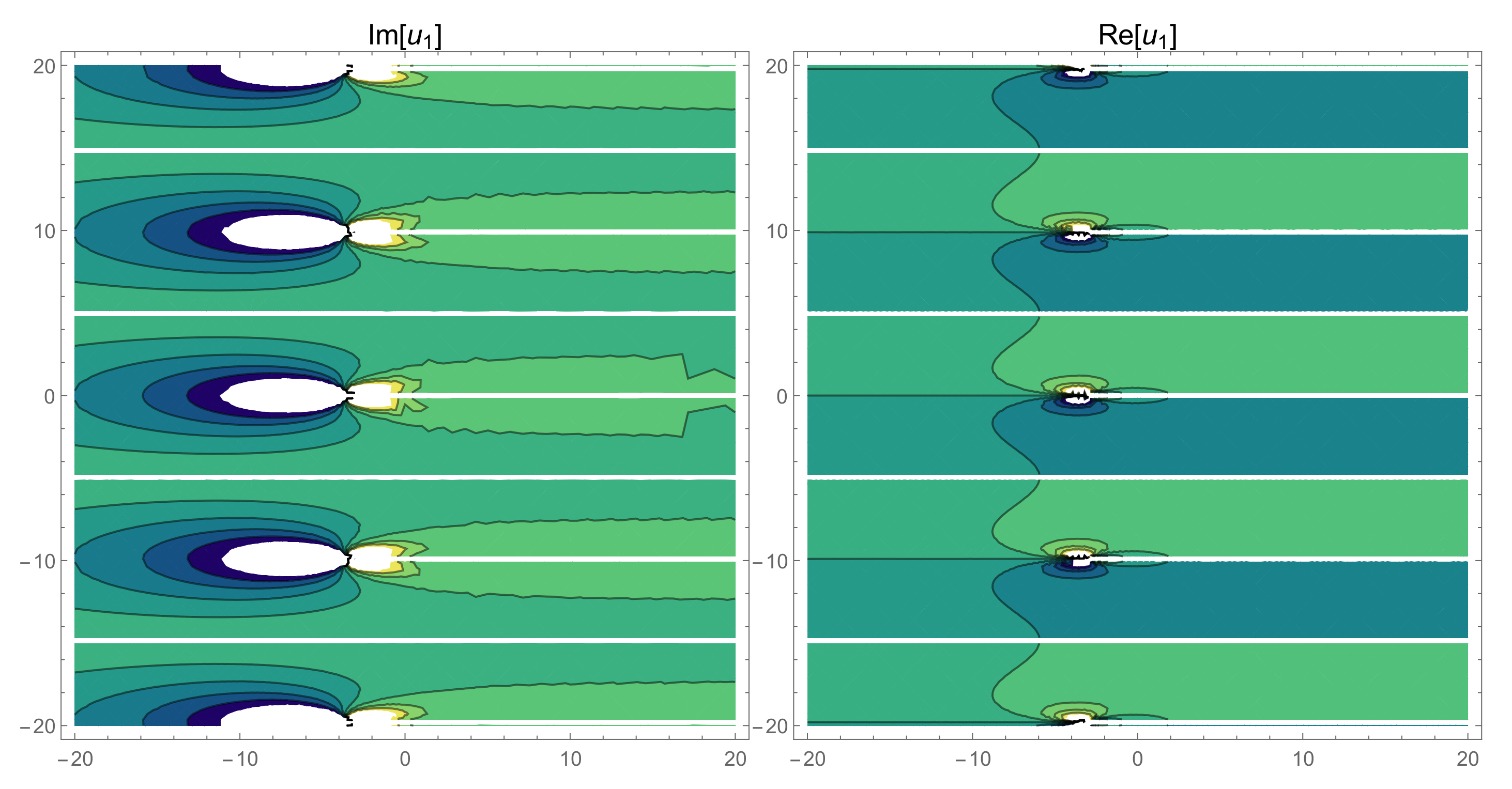
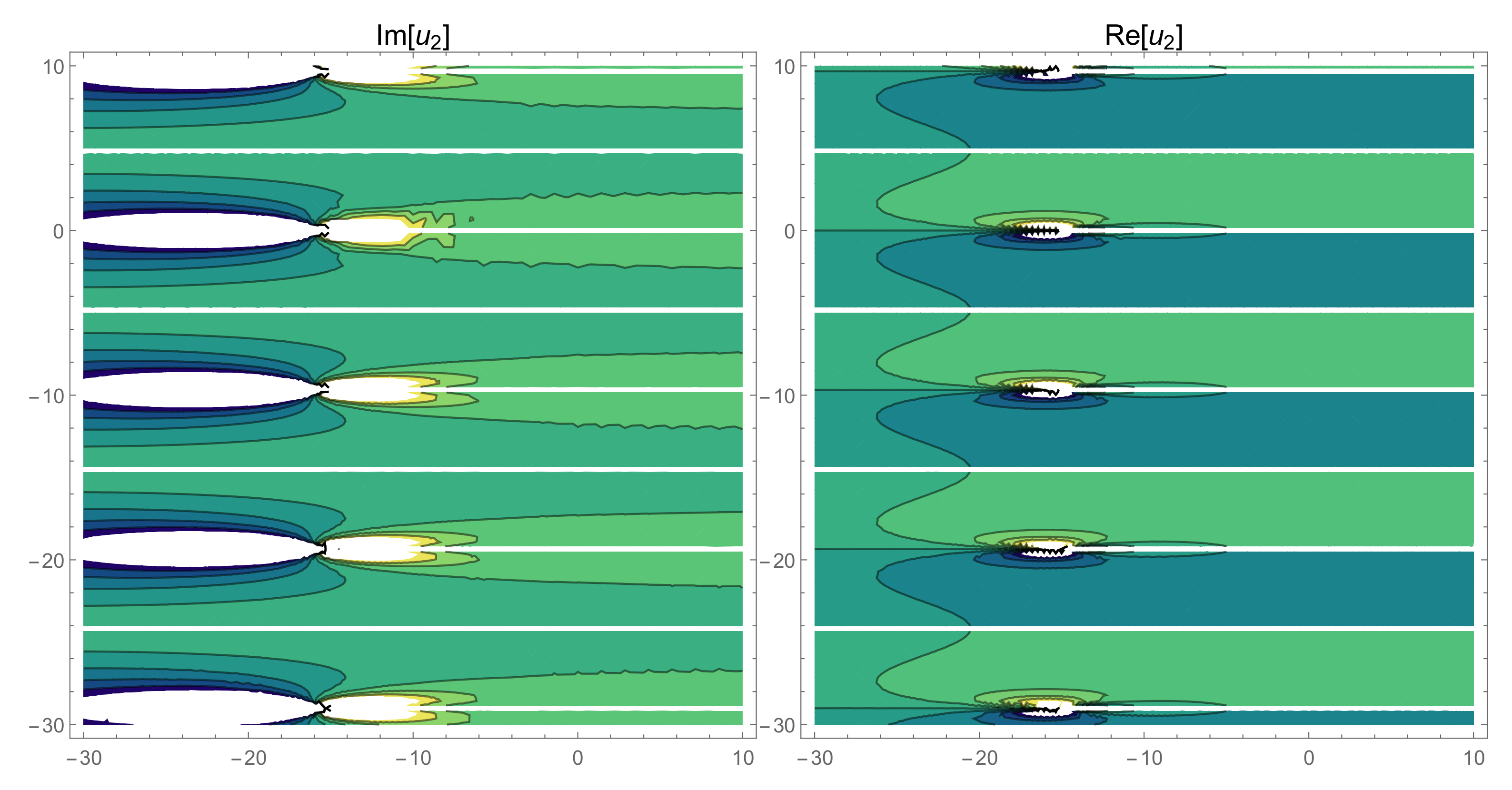
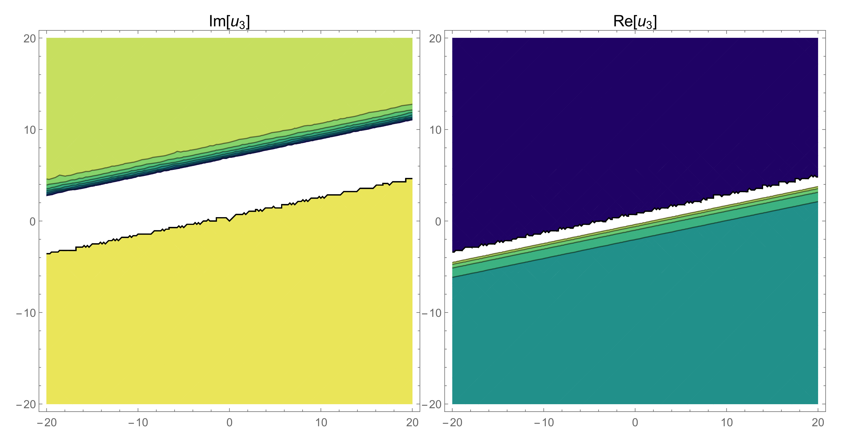
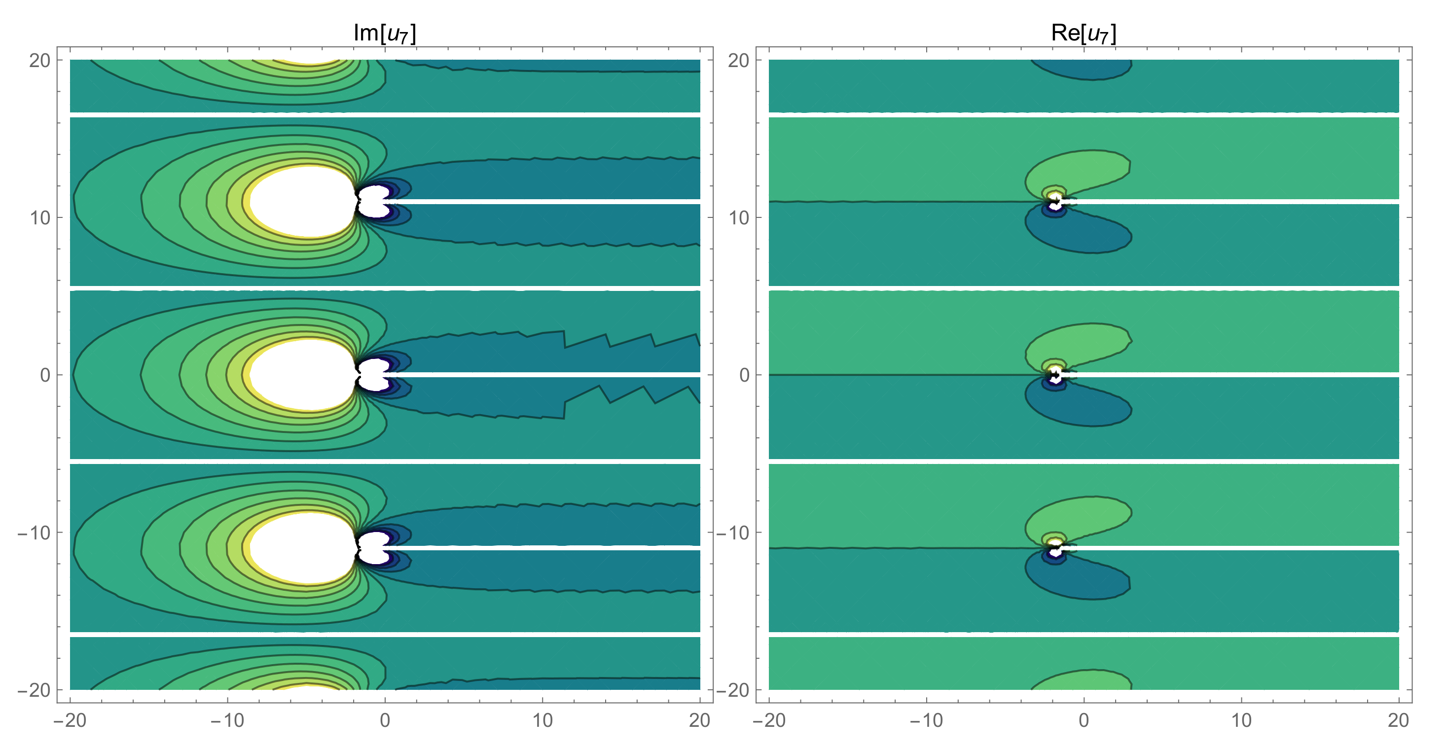
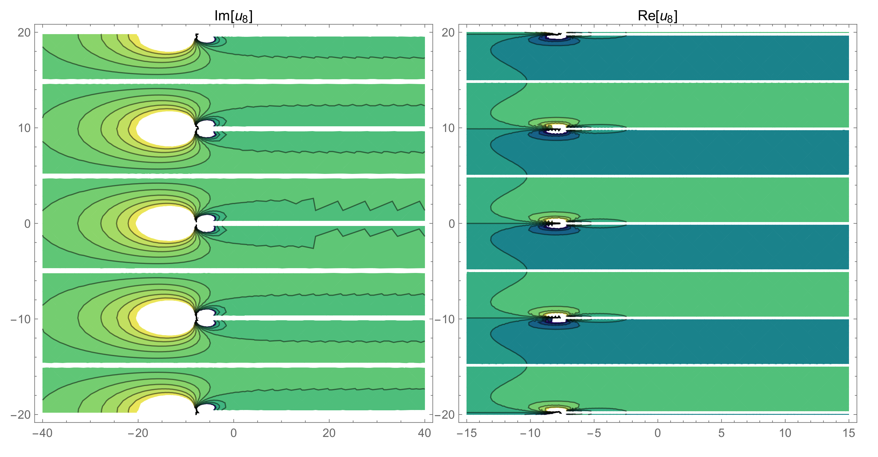
4. The Physical Properties

Recently, with the developing technological improvements in applied sciences, many real world problems are symbolized by using mathematical models. Traditional methods may not be given the necessary solutions of these newly presented models. In such a circumstance, these methods need to be developed or modified. In this work, we tried to find more complex solutions of the nonlinear perturbed sine-Gordon equation. This model is used to explain some important properties of the Josephson effect. Therefore, results may be used to explain some deep properties of the Josephson effect in a complex domain. From the physical point of view, while some solutions of Equations (13), (14) and (18)–(21) are complex and periodic, solution (15) is singular and (16) is a hyperbolic function and finally solution (22) is an exponential function. From Figure 1, Figure 2, Figure 3, Figure 4, Figure 5, Figure 6, Figure 7, Figure 8, Figure 9, Figure 10, Figure 11, Figure 12, Figure 13, Figure 14 and Figure 15, it is observed that these new complex solutions are used to symbolize currents in the frame of the Josephson effect. Comparing the existing papers in the literature [10], it may be seen that these are new analytical solutions. Therefore, it is estimated that these results may be used to explain more information about the Josephson effect, which produces a current known as a supercurrent. Thus, these complex solutions are used to investigate another kind of property of the Josephson effect.

5. Some Remarks and Discussion

The main advantage of the method applied in this paper is to construct many parameters which produce new types of solutions to the governing model. It also has various strain conditions, such as parameter values, balance and satisfying the model. Moreover, this method is based on the Bernoulli differential equation. Therefore, the scheme needs to satisfy the necessary conditions of the Bernoulli model. From a theoretical point of view, in this paper, if we take the higher values of M and n which are in relationship of M and n coming from balance, such as M = 7 and n = 9 , the test function solution formula for Equation (5) may be obtained as:
U ( ξ ) = a 0 + a 1 F + a 2 F 2 + a 3 F 3 + a 4 F 4 + a 5 F 5 + a 6 F 6 + a 7 F 7 + a 8 F 8 + a 9 F 9 .
In this equation, F has the analytical solutions of the Bernoulli differential equation given by F = b F + d F 7 , where F is F ( ξ ) . Comparing previous cases in this paper, we have more parameters such as a 7 , a 8 , a 9 . These parameters may be used to produce many new types of solutions such as trigonometric, periodic, travelling, dark, bright, mixed dark–bright and complex soliton solutions to the nonlinear mathematical models. These parameters extract deeper properties of the model considered.

6. Conclusions

In this study, the nonlinear perturbed sine-Gordon equation was studied under the norms method applied. We found many different types of solution to the governing model containing the Josephson effect. The main criterion used to measure accuracy is to satisfy the model and simulate the wave behavior of the dependant variable. In this frame, it is seen that all solutions satisfied the model. The strain conditions for valid solutions are also reported. The obtained solutions are illustrated by using figures under the suitably chosen parameters. The algorithm of scheme and figures are produced via a computational package program, namely, Mathematica. When these results obtained in this paper are compared with existing solutions in the literature, it is estimated that these are used to explain the different properties of the phase difference of the electrons. These results may be used to explain the special properties of the Josephson effect in the frame of impedance between two superconductors [25]. Especially, from Figure 1, Figure 4 and Figure 14, the Josephson effect may be clearly observed from the left side of x. Such simulations are based on the theoretical aspect of the method. The limitation of the proposed method is based on the calculation of parameters. If we obtain more values of M and n, we find more equations for the system of equations. This is the main advantage of the method used in this paper. From the solutions and figures, it may be estimated that such results may help to explain the Josephson effect by using complex norms. Moreover, this scheme may also be applied to other models in [26,27,28,29,30,31,32] as a future direction of the study. It can be inferred from the results that the method may be highly efficient for solving real world problems arising in the fields of engineering and applied science [26,27,28,29,30,31,32,33,34,35,36,37,38,39,40,41,42,43,44,45,46,47,48,49].

Author Contributions

Conceptualization, J.L.G.G. and H.M.B.; methodology, G.R.B.; investigation, F.S.V.C. All authors have read and agreed to the published version of the manuscript.

Funding

This research received no external funding.

Institutional Review Board Statement

This paper was partially supported by King Abdulaziz University with project ID: KEP-1-130-38.

Data Availability Statement

Not applicable.

Conflicts of Interest

The authors declare no conflict of interest.

References

  1. Josephson, B.D. Possible new effects in superconductive tunnelling. Phys. Lett. 1962, 1, 251–253. [Google Scholar] [CrossRef]
  2. Josephson, B.D. The discovery of tunnelling supercurrents. Rev. Mod. Phys. 1974, 46, 251–254. [Google Scholar] [CrossRef] [Green Version]
  3. Available online: https://www.britannica.com/biography/Brian-Josephson (accessed on 1 January 2020).
  4. Anderson, P.W.; Rowell, J.M. Probable Observation of the Josephson Tunnel Effect. Phys. Rev. Lett. 1963, 10, 230. [Google Scholar] [CrossRef]
  5. Zharkov, G.F. The Josephson Tunneling Effect In Superconductors. Soviet Physics Uspekhi 1966, 9, 1–13. [Google Scholar] [CrossRef]
  6. Pankratov, A.L.; Sobolev, A.S.; Koshelets, V.P.; Mygind, J. Influence of surface losses and the self-pumping effect on current-voltage characteristics of a long Josephson junction. Phys. Rev. B 2007, 75, 184516. [Google Scholar] [CrossRef] [Green Version]
  7. Pankratov, A.L. Long Josephson junctions with spatially inhomogeneous driving. Phys. Rev. B 2002, 66, 134526. [Google Scholar] [CrossRef] [Green Version]
  8. Pankratov, A.L. Noise self-pumping in long Josephson junctions. Phys. Rev. B 2008, 78, 024515. [Google Scholar] [CrossRef]
  9. Ha, J.; Nakagiri, S.I. Identification of constant parameters in perturbed sine-Gordon equations. J. Korean Math. Soc. 2006, 43, 931–950. [Google Scholar] [CrossRef] [Green Version]
  10. Guckenheimer, J.; Holmes, P. Nonlinear Oscillations, Dynamical Systems and Bifurcations of Vector Fields; Springer: New York, NY, USA, 1983. [Google Scholar]
  11. Barone, A.; Paternò, G. Physics and Applications of the Josephson Effect; John Wiley and Sons, Inc.: New York, NY, USA, 1982. [Google Scholar]
  12. Scott, A.C.; Chu, F.Y.F.; Reible, S.A. Magnetic flux propagation on a Josephson transmission line. J. Appl. Phys. 1976, 47, 3272–3286. [Google Scholar] [CrossRef]
  13. Derks, G.; Doelman, A.; van Gils, S.A.; Visser, T. Travelling waves in a singularly perturbed sine-Gordon equation. Physica D 2003, 180, 40–70. [Google Scholar] [CrossRef] [Green Version]
  14. Kivshar, Y.S.; Malomed, B.A. Many-particle effects in nearly integrable systems. Physica D 1987, 24, 125–154. [Google Scholar] [CrossRef]
  15. Kivshar, Y.S.; Malomed, B.A. Dynamics of solitons in nearly integrable systems. Rev. Mod. Phys. 1989, 61, 763–915. [Google Scholar] [CrossRef]
  16. Ha, J.H.; Nagiri, S. Identification problems of damped sine-gordon equations with constant parameters. J. Korean Math. Soc. 2002, 39, 509–524. [Google Scholar] [CrossRef]
  17. Lions, J.L.; Magenes, E. Non-Homogeneous Boundary Value Problems and Applications; Springer: New York, NY, USA; Heildelberg, Germany, 1972; Volume II. [Google Scholar]
  18. Sasaki, A.; Ikegaya, S.; Habe, T.; Golubov, A.A.; Asano, Y. Josephson effect in two-band superconductors. Phys. Rev. B 2020, 101, 184501. [Google Scholar] [CrossRef]
  19. Pagano, S. Introduction to Weak Superconductivity Josephson Effect: Physics and Applications; Lecture Notes; Springer: New York, NY, USA, 2020. [Google Scholar]
  20. Seidel, P. 8-High-Tc Josephson junctions. High-Temp. Supercond. 2011, 317–369. [Google Scholar] [CrossRef]
  21. Couëdo, F.; Amari, P.; Palma, C.F.; Ulysse, C.; Rivastava, Y.K.S.; Singh, R.; Bergeal, N.; Lesueur, J. Dynamic properties of high-Tc superconducting nano-junctions made with a focused helium ion beam. Sci. Rep. 2020, 10, 10256. [Google Scholar] [CrossRef]
  22. Zheng, B. Application of A Generalized Bernoulli Sub-ODE Method For Finding Traveling Solutions of Some Nonlinear Equations. WSEAS Trans. Math. 2012, 7, 618–626. [Google Scholar]
  23. Baskonus, H.M.; Mahmud, A.A.; Muhamad, K.A.; Tanriverdi, T. A study on Coudrey-Dodd-Gibbon-Sawada-Kotera partial differential equation. Math. Methods Appl. Sci. 2022. [Google Scholar] [CrossRef]
  24. Gao, W.; Baskonus, H.M.; Mahmud, A.A.; Muhamad, K.A.; Tanriverdi, T. Studing on kudryashov-sinelshchıkov dynamical equation arising in mixtures liquid and gas bubbles. Therm. Sci. 2022, 26, 1229–1244. [Google Scholar]
  25. Weisstein, E.W. Concise Encyclopedia of Mathematics, 2nd ed.; CRC Press: New York, NY, USA, 2002. [Google Scholar]
  26. Wang, K.J. Abundant exact soliton solutions to the Fokas system. Optik 2022, 249, 168265. [Google Scholar] [CrossRef]
  27. Wang, K.J. Abundant analytical solutions to the new coupled Konno-Oono equation arising in magnetic field. Results Phys. 2021, 31, 104931. [Google Scholar] [CrossRef]
  28. Wang, K.J.; Wang, G. Exact traveling wave solutions for the system of the ion sound and Langmuir waves by using three effective methods. Results Phys. 2022, 35, 105390. [Google Scholar] [CrossRef]
  29. Wang, K.J.; Wang, G. Variational theory and new abundant solutions to the (1+2)-dimensional chiral nonlinear Schrödinger equation in optics. Phys. Lett. A 2021, 412, 127588. [Google Scholar] [CrossRef]
  30. Wang, K.J. Jing Si, Investigation into the Explicit Solutions of the Integrable (2+1)-Dimensional Maccari System via the Variational Approach. Axioms 2022, 11, 234. [Google Scholar] [CrossRef]
  31. Wang, K.J.; Shi, F.; Liu, J.H.; Si, J. Application of the extended F-expansion method for solving the fractional Gardner equation with conformable fractional derivative. Fractal 2022. [Google Scholar] [CrossRef]
  32. Wang, K.J. Traveling wave solutions of the Gardner equation in dusty plasmas. Results Phys. 2022, 33, 105207. [Google Scholar] [CrossRef]
  33. Sulaiman, T.A.; Bulut, H.; Baskonus, H.M. On the exact solutions to some system of complex nonlinear models. Appl. Math. Nonlinear Sci. 2020, 6, 29–42. [Google Scholar] [CrossRef]
  34. Baskonus, H.M.; Bulut, H.; Sulaiman, T.A. New Complex Hyperbolic Structures to the Lonngren-Wave Equation by Using Sine-Gordon Expansion Method. Appl. Math. Nonlinear Sci. 2019, 4, 141–150. [Google Scholar] [CrossRef] [Green Version]
  35. Frassu, S.; Viglialoro, G. Boundedness criteria for a class of indirect (and direct) chemotaxis-consumption models in high dimensions. Appl. Math. Lett. 2022, 132, 108108. [Google Scholar] [CrossRef]
  36. Baskonus, H.M.; Kayan, M. Regarding new wave distributions of the nonlinear integro-partial ITO differential and fifth-order integrable equations. Appl. Math. Nonlinear Sci. 2021, 1–20. [Google Scholar] [CrossRef]
  37. Yu, X.Q.; Kong, S. Travelling wave solutions to the proximate equations for LWSW. Appl. Math. Nonlinear Sci. 2021, 6, 335–346. [Google Scholar] [CrossRef]
  38. Gao, W.; Ismael, H.F.; Husien, A.M.; Bulut, H.; Baskonus, H.M. Optical Soliton solutions of the Nonlinear Schrodinger and Resonant Nonlinear Schrodinger Equation with Parabolic Law. Appl. Sci. 2020, 10, 219. [Google Scholar] [CrossRef] [Green Version]
  39. Li, T.; Viglialoro, G. Boundedness for a nonlocal reaction chemotaxis model even in the attraction-dominated regime. Diff. Int. Equ. 2021, 34, 315–336. [Google Scholar]
  40. Uddin, M.F.; Hafez, M.G.; Hammouch, Z.; Rezazadeh, H.; Baleanu, D. Traveling wave with beta derivative spatial-temporal evolution for describing the nonlinear directional couplers with metamaterials via two distinct methods. Alex. Eng. J. 2021, 60, 1055–1065. [Google Scholar] [CrossRef]
  41. Uddin, M.F.; Hafez, M.G.; Hammouch, Z.; Baleanu, D. Periodic and rogue waves for Heisenberg models of ferromagnetic spin chains with fractional beta derivative evolution and obliqueness. Waves Random Complex Media 2020, 31, 2135–2149. [Google Scholar] [CrossRef]
  42. Greco, A.; Viglialoro, G. Existence and Uniqueness for a Two-Dimensional Ventcel Problem Modeling the Equilibrium of a Prestressed Membrane. Appl. Math. 2022. [Google Scholar] [CrossRef]
  43. Bulut, H.; Akkilic, A.N.; Khalid, B.J. Soliton solutions of Hirota equation and Hirota-Maccari system by the (m+1/G’)-expansion method. Adv. Math. Model. Appl. 2021, 6, 22–30. [Google Scholar]
  44. Xu, L.; Aouad, M. Application of Lane-Emden differential equation numerical method in fair value analysis of financial accounting. Appl. Math. Nonlinear Sci. 2022. [Google Scholar] [CrossRef]
  45. Ciancio, A.; Ciancio, V.; Onofrio, A.; Flora, B.F.F. A Fractional Model of Complex Permittivity of Conductor Media with Relaxation: Theory vs. Experiments. Fractal Fract. 2022, 6, 390. [Google Scholar] [CrossRef]
  46. Ciancio, A.; Ciancio, V.; Franccesso, F. Wave propagation in media obeying a thermoviscoanelastic model. U.P.B. Sci. Bull. Ser. A 2007, 69, 69–79. [Google Scholar]
  47. Ciancio, A.; Yel, G.; Kumar, A.; Baskonus, H.M.; Ilhan, E. On the complex mixed dark-bright wave distributions to some conformable nonlinear integrable models. Fractals 2022, 30, 2240018. [Google Scholar] [CrossRef]
  48. Ramos, H.; Rufai, M.A. An adaptive one-point second-derivative Lobatto-type hybrid method for solving efficiently differential systems. Int. J. Comput. Math. 2022, 99, 1687–1705. [Google Scholar] [CrossRef]
  49. Duromola, M.K.; Momoh, A.L.; Rufai, M.A.; Animasaun, I.L. Insight into 2-step continuous block method for solving mixture model and SIR model. Int. J. Comput. Sci. Math. 2021, 14, 347–356. [Google Scholar] [CrossRef]
Figure 1. The 3D figures of Equation (13).
Mathematics 10 02591 g001
Figure 2. The contour figures of Equation (13).
Mathematics 10 02591 g002
Figure 3. The 2D figures of Equation (13).
Mathematics 10 02591 g003
Figure 4. The 3D figures of Equation (14).
Mathematics 10 02591 g004
Figure 5. The contour figures of Equation (14).
Mathematics 10 02591 g005
Figure 6. The 2D figures of Equation (14).
Mathematics 10 02591 g006
Figure 7. The 3D figures of Equation (15).
Mathematics 10 02591 g007
Figure 8. The contour figures of Equation (15).
Mathematics 10 02591 g008
Figure 9. The 3D figures of Equation (18).
Mathematics 10 02591 g009
Figure 10. The contour figures of Equation (18).
Mathematics 10 02591 g010
Figure 11. The 2D figures of Equation (18).
Mathematics 10 02591 g011
Figure 12. The 3D figures of Equation (20).
Mathematics 10 02591 g012
Figure 13. The contour figures of Equation (20).
Mathematics 10 02591 g013
Figure 14. The 2D figures of Equation (20).
Mathematics 10 02591 g014
Figure 15. The 3D figures of Equation (21).
Mathematics 10 02591 g015
Figure 16. The contour figures of Equation (21).
Mathematics 10 02591 g016
Table 1. Meanings of parameters.
ParametersMeanings
γ The applied bias current
α u t The ohmic losses term
β u x x t The surface losses term
ϵ The term for definiteness
Publisher’s Note: MDPI stays neutral with regard to jurisdictional claims in published maps and institutional affiliations.

