Partial Least Squares Regression for Binary Responses and Its Associated Biplot Representation

Abstract

In this paper, we propose a generalization of Partial Least Squares Regression (PLS-R) for a matrix of several binary responses and a a set of numerical predictors. We call the method Partial Least Squares Binary Logistic Regression (PLS-BLR). That is equivalent to a PLS-2 model for binary responses. Biplot and even triplot graphical representations for visualizing PLS-BLR models are described, and an application to real data is presented. Software packages for the calculation of the main results are also provided. We conclude that the proposed method and its visualization using triplots are powerful tools for the interpretation of the relations among predictors and responses.

1. Introduction

We have an $I\times J$ data matrix $\mathbf{X}$ $=\left(x_{ij}\right)$ with the values of J predictor variables and an $I\times K$ matrix $\mathbf{Y}$ $=\left(y_{ik}\right)$ with the values of K response variables. Then, we have I individuals, J predictors and K responses.

Scientific modelling often involves using a set of predictors or explanatory variables to explain, regulate or predict the behaviour of a set of responses. Partial Least Squares Regression (PLS-R) is a popular method for modelling the relationships among both sets, especially in industrial or chemometric applications [1] when both contain continuous variables. When the predictors are few and have no redundant effects, multiple or multivariate linear regression (MLR) could be used to model the behaviour of responses; however, if some application conditions do not hold, those models are not appropriate. An interesting particular example is when the number of observations is much smaller than the number of predictors; then, the parameter estimates for the MLR do not exist. That is the case, for example, in genomic studies where a set of gene expressions may be used to predict the type of tumour.

PLS-R is a method for constructing models when there are a high number of predictors, or they are highly collinear, see [2,3]. For example. PLS-R is used mainly for prediction and is not considered as an appropriate procedure for understanding the underlying relationships among the variables although together with a suitable graphical representation it can provide information about the structure of the data. We state here that a biplot is such a representation. Ref. [4] proposes a biplot representation for the PLS solution when the responses are continuous although previous less formal versions can be found, for example, in [5] among some other authors. Recently, ref. [6] applied the PLS-Biplot to team effectiveness data.

For a binary response, PLS Discriminant Analysis (PLS-DA)  [7] that basically fits a PLS-R to a dummy variable is used. The reasoning behind that is similar to the relationship between Canonical Correlation Analysis and Discriminant Analysis, the second being a particular case of the first when one of the sets is formed by dummy or indicator variables.

In the regression case, we could use Logistic Regression (LR) for discrimination, capturing the binary nature of the response, although LR has the same limitations as MLR in relation to the number of individuals and variables or collinearity, with additional problems when there is a perfect prediction.

The objective of this work is to generalise the usual PLS-R to cope with multiple binary responses using logistic rather than linear functions. That would also be an alternative to the PLS-DA analysis in the same way as LR is an alternative to Discriminant Analysis. In [8], there is a generalization for a single binary response variable, but when there are several variables, it is necessary to reduce the dimension of the binary data, i.e., we want to develop a PLS-2 (PLS with more than two responses) version for binary dependent variables. Together with the model, we want a pictorial representation of the results.

In this paper, we propose the PLS-R method for the case when there is a set of binary dependent variables, using logistic rather than linear fits to take into account the nature of responses. We term the method PLS-BLR (Partial Least Squares Binary Logistic Regression). This is a generalization to several binary responses of the model in [8].

A triplot (a joint representation of individuals and response and explanatory variables) is used to assess the quality of predictions visually and to recognize the variables associated to them. The resulting triplot will be a combination of a traditional representation for numeric data and a Logistic Biplot as described by [9,10]. The procedure is also an extension of the Redundancy Analysis for Binary responses recently proposed by [11], the main difference being that in the previous procedure the dimension reduction is just for the responses, while in this it is for both sets.

First, we describe the base methods, PLS-R and its associated biplots, then PLS-BLR as a generalization of PLS-R for binary responses and its associated triplot. The procedures proposed here are descriptive, used for visualization, in the sense that we do not provide measures of the variability of the parameters. Finally, we will apply the method to two sets of real data: the first related to the classification of Spanish wines and the second related to environmental variables among species.

2. PLS-R: The NIPALS Algorithm

In this section, we describe partial least squares regression when both sets, responses and predictors are continuous numerical variables.

2.1. PLS-R

The purpose of PLS-R is predicting $\mathbf{Y}$ from $\mathbf{X}$ and describing its common structure. It is different from Multiple Regression (MR) in that $\mathbf{X}$ does not have to be of full rank. That is the case, for example, when the amount of independent variables is higher than the number of individuals or the variables are highly collinear. A possible solution of the problem would be using the Principal Components (PC) as predictors, but there is no guarantee that the PCs are adequate to explain the responses. The PLS models find two sets of new variables that are linear combinations of the predictors. The first set is the response variables. The second set is configured in such a way that the new composite variables catch the relationships among the two data matrices as well as possible. PLS-R combines features of MLR and PC obtaining components from $\mathbf{X}$ that are relevant to predict $\mathbf{Y}$.

NIPALS Algorithm

PLS aims to find a linear combination of the predictors $\mathbf{X}$ that best predict the responses $\mathbf{Y}$. We describe the classical NIPALS algorithm here [12]. When data are continuous, both sets are usually column-centred.

The matrix $\mathbf{X}$ can be decomposed as

$$\mathbf{X}=\mathbf{T}{\mathbf{P}}^T+\mathbf{E}=E\left[\mathbf{X}\right]+\mathbf{E}=\widehat{\mathbf{X}}+\mathbf{E},$$

(1)

where $\mathbf{P}$ is the $J\times S$ matrix of loadings, $\mathbf{T}$ is a $I\times S$ matrix of scores and $\mathbf{E}$ is a $I\times J$ matrix of residuals.

In the same way, we can decompose the matrix $\mathbf{Y}$ as

$$\mathbf{Y}=\mathbf{T}{\mathbf{Q}}^T+\mathbf{F}=E\left[\mathbf{Y}\right]+\mathbf{F}=\widehat{\mathbf{Y}}+\mathbf{F},$$

(2)

where $\mathbf{Q}$ is the $K\times S$ matrix of loadings, $\mathbf{T}$ is a $I\times S$ matrix of scores and $\mathbf{F}$ is a $I\times K$ matrix of residuals. Note that both decompositions are similar to a principal components analysis or a biplot of each matrix. If we want separate decompositions, we can use the NIPALS algorithm for principal components [13]. The common set of scores $\mathbf{T}$ is used as predictors in the modelling of $\mathbf{Y}$ and is obtained from $\mathbf{X}$.

For the matrix $\mathbf{X}$ we have Algorithm 1:

Algorithm 1 X-Components Algorithm
1:	procedure X-Components ($\mathbf{X},S$)
2:	for $s=1\to S$ do
3:	${\mathbf{t}}_{\left(s\right)}\leftarrow {\mathbf{x}}_{\left(j\right)}$ for some j	▹ Init: ${\mathbf{t}}_{\left(s\right)}$
4:	repeat
5:	${\mathbf{p}}_{\left(s\right)}\leftarrow {\mathbf{X}}^T{\mathbf{t}}_{\left(s\right)}/\Vert {\mathbf{X}}^T{\mathbf{t}}_{\left(s\right)}\Vert$	▹ Update: ${\mathbf{p}}_{\left(s\right)}$
6:	${\mathbf{t}}_{\left(s\right)}\leftarrow {\mathbf{Xp}}_{\left(s\right)}$	▹ Update: ${\mathbf{t}}_{\left(s\right)}$
7:	until ${\mathbf{t}}_{\left(s\right)}$ does not change
8:	$\mathbf{X}\leftarrow \mathbf{X}-{\mathbf{t}}_{\left(s\right)}{\mathbf{p}}_{\left(s\right)}^T$	▹ Update: $\mathbf{X}$
	return $\mathbf{T}=\left[{\mathbf{t}}_{\left(1\right)}, \dots , {\mathbf{t}}_{\left(S\right)}\right]$ and $\mathbf{P}=\left[{\mathbf{p}}_{\left(1\right)}, \dots , {\mathbf{p}}_{\left(S\right)}\right]$

For the matrix $\mathbf{Y}$, the algorithm would be the same as Algorithm 1 (X-Components), substituting $\mathbf{X}$ by $\mathbf{Y}$ and $\mathbf{P}=\left[{\mathbf{p}}_{\left(1\right)}, \dots , {\mathbf{p}}_{\left(S\right)}\right]$ by $\mathbf{Q}=\left[{\mathbf{q}}_{\left(1\right)}, \dots , {\mathbf{q}}_{\left(S\right)}\right]$.

In this case, $\widehat{\mathbf{X}}$ and $\widehat{\mathbf{Y}}$ are lower rank (S) approximations of $\mathbf{X}$ and $\mathbf{Y}$, respectively. According to [13], ${\mathbf{p}}_{\left(s\right)}$ is an eigenvector of ${\mathbf{X}}^T\mathbf{X}$ and the algorithm is a variant of the power method for matrix diagonalization as described, for example, in [14]. One of the advantages over the singular value decomposition (SVD) is that while SVD calculates all the principal components simultaneously, NIPALS does it sequentially. For big data sets, the first alternative is prohibitive, while the second is more efficient. On the other hand, NIPALS loses the orthogonality because of the rounding errors, and it is useful only to obtain a few components [15].

Because we want to relate both sets of data, we can construct a combination of both procedures (for $\mathbf{X}$ and $\mathbf{Y}$) to obtain the NIPALS algorithm for PLS-R. This is in Algorithm 2.

Algorithm 2 NIPALS Algorithm
1:	procedure XY-Components ($\mathbf{X},\mathbf{Y},S$)
2:	for $s=1\to S$ do
3:	${\mathbf{t}}_{\left(s\right)}\leftarrow {\mathbf{y}}_{\left(j\right)}$ for some j	▹ Init: ${\mathbf{u}}_{\left(s\right)}$
4:	repeat
5:	${\mathbf{p}}_{\left(s\right)}\leftarrow {\mathbf{X}}^T{\mathbf{t}}_{\left(s\right)}/\Vert {\mathbf{X}}^T{\mathbf{t}}_{\left(s\right)}\Vert$	▹ Update: ${\mathbf{p}}_{\left(s\right)}$
6:	${\mathbf{t}}_{\left(s\right)}\leftarrow {\mathbf{Xp}}_{\left(s\right)}$	▹ Update: ${\mathbf{t}}_{\left(s\right)}$
7:	${\mathbf{q}}_{\left(s\right)}\leftarrow {\mathbf{Y}}^T{\mathbf{t}}_{\left(s\right)}/\Vert {\mathbf{Y}}^T{\mathbf{t}}_{\left(s\right)}\Vert$	▹ Update: ${\mathbf{q}}_{\left(s\right)}$
8:	${\mathbf{t}}_{\left(s\right)}\leftarrow {\mathbf{Yq}}_{\left(s\right)}$	▹ Update: ${\mathbf{t}}_{\left(s\right)}$
9:	until ${\mathbf{t}}_{\left(s\right)}$ does not change
10:	$\mathbf{X}\leftarrow \mathbf{X}-{\mathbf{t}}_{\left(s\right)}{\mathbf{p}}_{\left(s\right)}^T$	▹ Update: $\mathbf{X}$
11:	$\mathbf{Y}\leftarrow \mathbf{Y}-{\mathbf{t}}_{\left(s\right)}{\mathbf{q}}_{\left(s\right)}^T$	▹ Update: $\mathbf{Y}$
	return $\mathbf{T}=\left[{\mathbf{t}}_{\left(1\right)}, \dots , {\mathbf{t}}_{\left(S\right)}\right]$, $\mathbf{P}=\left[{\mathbf{p}}_{\left(1\right)}, \dots , {\mathbf{p}}_{\left(S\right)}\right]$ and $\mathbf{Q}=\left[{\mathbf{q}}_{\left(1\right)}, \dots , {\mathbf{q}}_{\left(S\right)}\right]$

Then, with this algorithm, ${\mathbf{P}}^T\mathbf{P}=\mathbf{I}$ and ${\mathbf{Q}}^T\mathbf{Q}=\mathbf{I}$ and $\mathbf{T}$ contain the scores of the $\mathbf{X}$’s that better explain the set of responses. We have that

$$\mathbf{T}=\mathbf{X}\mathbf{P}.$$

(3)

A potential problem of this and the following algorithms is that they may have various start points and then have different solutions. The algorithm produces sequences of decreasing values of the sum of squares of the residuals and then converge at least to a local minima.

If we want the regression coefficients for obtaining the $\mathbf{Y}$ variables as functions of the $\mathbf{X}$ variables

$$E\left[\mathbf{Y}\right]=\widehat{\mathbf{Y}}=\mathbf{X}\mathbf{B}.$$

(4)

Taking into account that $\widehat{\mathbf{Y}}=\mathbf{T}\mathbf{Q}$, we have

$$\widehat{\mathbf{Y}}=\mathbf{T}{\mathbf{Q}}^T=\mathbf{XP}\mathbf{Q}.$$

(5)

Then, the regression coefficients, in terms of the original variables, are

$$\mathbf{B}=\mathbf{P}{\mathbf{Q}}^T.$$

(6)

3. PLS Binary Logistic Regression

When the responses are binary, the linear model is not always the most adequate, and the regression equation in (2) has to be adapted using the logit transformation. Bastien et al. [8] propose a PLS model for a single binary response (the equivalent to a PLS-1 model). We extend the model to cope with several responses including a dimension reduction for the binary data, obtaining a PLS-2 model for binary variables based on logistic responses that has not previously been proposed in the literature. The method is also an alternative to the PLS-DA.

Here we will use a procedure similar to the method described in Algorithm 2 with the necessary adaptations to include binary data. The expected values are now probabilities, and we use the logit as a link function. Calling $E\left[\mathbf{Y}\right]=\mathbf{\Pi }$

$$\mathrm{logit}(\mathbf{\Pi })=\mathbf{1}{\mathbf{q}}_0^T+\mathbf{T}{\mathbf{Q}}^T.$$

(7)

The equation is a generalization of Equation (2) except that we have to add a vector ${\mathbf{q}}_0$ with intercepts for each variable. This is because binary variables cannot be centred as before. Each probability ${\pi }_{ik}$ can be written as

$${\pi }_{ik}=\frac{e^{\left(q_{k0} + {\sum }_{s=1}^S{t}_{ks}{q}_{ks}\right)}}{1+e^{\left(q_{k0} + {\sum }_{s=1}^S{t}_{ks}{q}_{ks}\right)}}.$$

(8)

Before generalising Algorithm 2, we have to generalise the part to cope with binary responses. Algorithm 1 can be kept as it is. The generalization for the separate components of the binary set is as follows.

3.1. Separate Components for the Binary Responses

For the responses, rather than using the residual sum of squares, we use

$$L=\sum _{i=1}^I\sum _{k=1}^K\left[-y_{ik}log\left({\pi }_{ik}\right)-(1-y_{ik})log\left(1-{\pi }_{ik}\right)\right],$$

(9)

as a cost function.

Observe that the function is essentially the reciprocal of maximum likelihood used to fit a standard logistic regression. Here we interpret the function as a cost to minimize rather than a likelihood to maximize.

We look for the parameters $\mathbf{T}$, $\mathbf{Q}$ and ${\mathbf{q}}_0$ that minimize the cost function. There are no closed-form solutions for the optimization problem, so an iterative algorithm in which we obtain a sequence of decreasing values of the lost function at each iteration is used. We will use the gradient method in a recursive way. The update for each parameter would be as follows:

$$q_{k0}=q_{k0}-\alpha \frac{\partial L}{\partial q_{k0}},t_{ks}=t_{ks}-\alpha \frac{\partial L}{\partial t_{ks}},q_{ks}=q_{ks}-\alpha \frac{\partial L}{\partial q_{ks}},$$

(10)

for a choice of $\alpha$.

The gradients for each parameter are

$$\frac{\partial L}{\partial q_{k0}}=\sum _{i=1}^I({\pi }_{ik}-y_{ik}),\frac{\partial L}{\partial t_{is}}=\sum _{k=1}^K{q}_{ks}({\pi }_{ik}-y_{ik}),\frac{\partial L}{\partial q_{ks}}=\sum _{i=1}^I{t}_{is}({\pi }_{ik}-y_{ik}).$$

(11)

We can organize the calculations in an alternated algorithm that alternatively calculates parameters for rows ${\mathbf{t}}_{\left(s\right)}=(t_{1s}, \dots , t_{Is})$ and columns ${\mathbf{q}}_{\left(s\right)}=(q_{1s}, \dots , q_{Ks})$ for each dimension s fixing the parameters already obtained for each previous dimensions as a way to obtain uncorrelated components. Before that, the constants ${\mathbf{q}}_{\left(0\right)}=(q_{10}, \dots , q_{K0})$ have to be fitted separately. The procedure would be as follows, in Algorithm 3.

Algorithm 3 Algorithm to calculate the Y-Components for Binary Data
1:	procedure Y-Binary-Components ($\mathbf{Y},S$)
2:	Choose $\alpha$
3:	${\mathbf{q}}_{\left(0\right)}=random$	▹ Init: ${\mathbf{q}}_{\left(0\right)}$
4:	repeat
5:	$q_{k0}\leftarrow q_{k0}-\alpha {\displaystyle \sum _{i=1}^I}(p_{ik}-y_{ik}), (k=1, \dots , K)$	▹ Update: ${\mathbf{q}}_{\left(0\right)}$
6:	${\pi }_{ik}\leftarrow \frac{e^{q_{k0}}}{1+e^{q_{k0}}}; (i=1, \dots , I; k=1, \dots , K)$	▹ Update: $\mathbf{\Pi }$
7:	until ${\mathbf{q}}_{\left(0\right)}$ do not change
8:	for $s=1\to S$ do
9:	${\mathbf{t}}_{\left(s\right)}\leftarrow random$	▹ Init: ${\mathbf{t}}_{\left(s\right)}$
10:	${\mathbf{q}}_{\left(s\right)}\leftarrow random$	▹ Init: ${\mathbf{q}}_{\left(s\right)}$
11:	repeat
12:	repeat
13:	$q_{ks}\leftarrow q_{ks}-\alpha {\displaystyle \sum _{k=1}^I}{t}_{is}({\pi }_{ik}-y_{ik})$	▹ Update: ${\mathbf{q}}_{\left(s\right)}$
14:	${\pi }_{ik}=\frac{e^{\left(q_{k0} + {\sum }_{l=1}^s{t}_{kl}{q}_{kl}\right)}}{1+e^{\left(q_{k0} + {\sum }_{l=1}^s{t}_{kl}{q}_{kl}\right)}}$	▹ Update: $\mathbf{\Pi }$
15:	until ${\mathbf{q}}_{\left(s\right)}$ do not change
16:	repeat
17:	$t_{is}\leftarrow t_{is}-\alpha {\displaystyle \sum _{k=1}^K}{q}_{ks}({\pi }_{ik}-y_{ik})$	▹ Update: ${\mathbf{t}}_{\left(s\right)}$
18:	${\pi }_{ik}=\frac{e^{\left(q_{k0} + {\sum }_{l=1}^s{t}_{kl}{q}_{kl}\right)}}{1+e^{\left(q_{k0} + {\sum }_{l=1}^s{t}_{kl}{q}_{kl}\right)}}$	▹ Update: $\mathbf{\Pi }$
19:	until ${\mathbf{t}}_{\left(s\right)}$ do not change
20:	$L\leftarrow {\displaystyle \sum _{i=1}^I}{\displaystyle \sum _{k=1}^K}\left[-y_{ik}log\left({\pi }_{ik}\right)-(1-y_{ik})log\left(1-{\pi }_{ik}\right)\right]$
21:	until L does not change
	return ${\mathbf{q}}_{\left(0\right)}=(q_{10}, \dots , q_{K0})$, $\mathbf{Q}=\left[{\mathbf{q}}_{\left(1\right)}, \dots , {\mathbf{q}}_{\left(S\right)}\right]$, $\mathbf{T}=\left[{\mathbf{t}}_{\left(1\right)}, \dots , {\mathbf{t}}_{\left(S\right)}\right]$

We can avoid the choice of $\alpha$ by using more complex procedures such as conjugate gradient. From the practical point of view, we can use optimization routines that will minimize the cost function in a much more efficient way. This should be enough for the purpose of this article. For more detailed and sophisticated procedures, see [16].

In practice, we do not have to use any particular value of $\alpha$, using general-purpose optimization packages in which just the cost and gradient functions are provided for the routines to work.

There may be another problem when fitting a logistic model known as the separation problem: when there is a hyperplane in the space generated by the $\mathbf{U}$’s that separate the presences and the absences, the estimates do not exist [17] and tend to infinity. Even when the separation is not perfect (quasi-separation), the estimates are highly unstable. The usual solution uses a penalized version of the cost function as in [18]. Here we could use a ridge penalization [19] as described later in the joint algorithm.

The algorithm has some random components at the start; therefore it may obtain different solutions. If each update decreases the value of the cost function, the algorithm will converge to a solution, which is at least a local minimum, hopefully the global minimum. Using several starting points can increase possibilities of obtaining the global minimum [20].

3.2. Algorithm PLS-BLR

Having set the methods to estimate the separated components, we can mix both procedures to obtain an algorithm for PLS-BLR that generalizes the NIPALS procedure shown before. First, we have to calculate the constant for the binary part because it is not possible to centre data as in the continuous case. Then we calculate the PLS components in a recursive way, combining Algorithms 1 and  3 in Algorithm 4 as follows:

Algorithm 4 PLS Binary Regression
1:	procedure PLS-BLR ($\mathbf{Y},S$)
2:	Choose $\alpha$
3:	${\mathbf{q}}_{\left(0\right)}=random$	▹ Init: ${\mathbf{q}}_{\left(0\right)}$
4:	repeat
5:	$q_{k0}\leftarrow q_{k0}-\alpha {\displaystyle \sum _{i=1}^I}(p_{ik}-y_{ik}), (k=1, \dots , K)$	▹ Update: ${\mathbf{q}}_{\left(0\right)}$
6:	${\pi }_{ik}\leftarrow \frac{e^{q_{k0}}}{1 + e^{q_{k0}}}; (i=1, \dots , I; k=1, \dots , K)$	▹ Update: $\mathbf{\Pi }$
7:	until ${\mathbf{q}}_{\left(0\right)}$ do not change
8:	for $s=1\to S$ do
9:	${\mathbf{t}}_{\left(s\right)}\leftarrow random$	▹ Init: ${\mathbf{t}}_{\left(s\right)}$
10:	${\mathbf{q}}_{\left(s\right)}\leftarrow random$	▹ Init: ${\mathbf{q}}_{\left(s\right)}$
11:	repeat
12:	${\mathbf{p}}_{\left(s\right)}\leftarrow {\mathbf{X}}^T{\mathbf{t}}_{\left(s\right)}/\Vert {\mathbf{X}}^T{\mathbf{t}}_{\left(s\right)}\Vert$	▹ Update: ${\mathbf{p}}_{\left(s\right)}$
13:	${\mathbf{t}}_{\left(s\right)}\leftarrow {\mathbf{Xp}}_{\left(s\right)}$	▹ Update: ${\mathbf{t}}_{\left(s\right)}$
14:	repeat
15:	$q_{ks}\leftarrow q_{ks}-\alpha {\displaystyle \sum _{k=1}^I}{u}_{is}({\pi }_{ik}-y_{ik})$	▹ Update: ${\mathbf{q}}_{\left(s\right)}$
16:	${\pi }_{ik}=\frac{e^{\left(q_{k0} + {\sum }_{l=1}^s{u}_{kl}{q}_{kl}\right)}}{1 + e^{\left(q_{k0} + {\sum }_{l=1}^s{u}_{kl}{q}_{kl}\right)}}$	▹ Update: $\mathbf{\Pi }$
17:	until ${\mathbf{q}}_{\left(s\right)}$ do not change
18:	repeat
19:	$t_{is}\leftarrow t_{is}-\alpha {\displaystyle \sum _{k=1}^K}{q}_{ks}({\pi }_{ik}-y_{ik})$	▹ Update: ${\mathbf{t}}_{\left(s\right)}$
20:	${\pi }_{ik}=\frac{e^{\left(q_{k0} + {\sum }_{l=1}^s{t}_{kl}{q}_{kl}\right)}}{1 + e^{\left(q_{k0} + {\sum }_{l=1}^s{t}_{kl}{q}_{kl}\right)}}$	▹ Update: $\mathbf{\Pi }$
21:	until ${\mathbf{t}}_{\left(s\right)}$ do not change
22:	$L\leftarrow {\displaystyle \sum _{i=1}^I}{\displaystyle \sum _{k=1}^K}\left[-y_{ik}log\left({\pi }_{ik}\right)-(1-y_{ik})log\left(1-{\pi }_{ik}\right)\right]$
23:	until L does not change
24:	$\mathbf{X}\leftarrow \mathbf{X}-{\mathbf{t}}_{\left(s\right)}{\mathbf{p}}_{\left(s\right)}^T$	▹ Update: $\mathbf{X}$
	return ${\mathbf{q}}_{\left(0\right)}=(q_{10}, \dots , q_{K0})$, $\mathbf{Q}=\left[{\mathbf{q}}_{\left(1\right)}, \dots , {\mathbf{q}}_{\left(S\right)}\right]$, $\mathbf{P}=\left[{\mathbf{p}}_{\left(1\right)}, \dots , {\mathbf{p}}_{\left(S\right)}\right]$ and $\mathbf{T}=\left[{\mathbf{t}}_{\left(1\right)}, \dots , {\mathbf{t}}_{\left(S\right)}\right]$

The procedure in Algorithm 4 may have the same problems as Algorithm 3 in relation to the separation problem. Actually, with many data sets in which a good fit for the responses is reached, the separation is likely to occur. In that case some of $\mathbf{Q}$ may tend to infinity.

A quadratic penalization could be used in the cost function

$$L=\sum _{i=1}^I\sum _{k=1}^K\left[-y_{ik}log\left({\pi }_{ik}\right)-(1-y_{ik})log\left(1-{\pi }_{ik}\right)\right]+\lambda \sum _{k=1}^K\sum _{s=1}^S{q}_{ks}^2.$$

(12)

The adaptation of the gradient is straightforward

$$\frac{\partial L}{\partial q_{ks}}=\sum _{i=1}^I{u}_{is}({\pi }_{ik}-y_{ik})+2\lambda q_{ks}.$$

(13)

Now there is another parameter ($\lambda$) that has to be tuned. The usual strategy is trying different values to select the optimum, although any positive value would be enough to solve the problem. A profile method is needed to find the optimal $\lambda$, for example, a grid $\lambda =(0.1, \dots , 100)$, and solve Equation (13).

The algorithm may also have problems in relation to the random start. It should produce decreasing values of the cost functions in both sets that converge at least to a local minimum. Several starting points can be tried to find the best solution. From our experience, the solutions for various starts have similar predictions of the responses.

3.3. Logistic Regression Model

As in the continuous case, we can now regress the columns of $\mathbf{Y}$ on $\mathbf{T}$ with a logistic regression. As we can see in Algorithm 1, ${\mathbf{q}}_0$ and $\mathbf{Q}$ contain the regression coefficients. In terms of the original variables

$$\mathrm{logit}(\mathbf{\Pi })=\mathbf{1}{\mathbf{q}}_0^T+\mathbf{T}{\mathbf{Q}}^T=\mathbf{1}{\mathbf{q}}_0^T+\mathbf{XPQ}.$$

(14)

Then

$$\mathrm{logit}(\mathbf{\Pi })=\mathbf{1}{\mathbf{q}}_0^T+\mathbf{X}{\mathbf{B}}^T,$$

(15)

with 6

$$\mathbf{B}=\mathbf{P}{\mathbf{Q}}^T,$$

(16)

i.e., $\mathbf{B}$ is the regression coefficients relative to the observed variables.

4. PLS Biplot

In this section, we discuss the construction of a biplot for the visualization of the results. Although biplots are well known, we describe some of its main characteristics that are related to our proposal here. The final representation will combine a classical biplot for the continuous predictors, together with a logistic biplot for the binary responses, both sharing the same scores for the individuals.

4.1. Biplot for Continuous Data

4.1.1. Prediction Biplot

It is well known that a given factorization of a matrix $\mathbf{X}\approx {\mathbf{A}\mathbf{B}}^T$ defines a biplot of $\mathbf{X}$ [21,22]. Normally, the factorization is related to PCA or SVD in such a way that the factorization, in reduced dimension (two or three), produces the best low rank approximation to $\mathbf{X}$ [21,22]. In this context, the biplot can also be obtained from Algorithm 1, leading to equivalent results ($\mathbf{A}=\mathbf{T}$ and $\mathbf{B}=\mathbf{P}$). The rows of $\mathbf{A}$ and $\mathbf{B}$ can be used as markers for the individuals and variables of $\mathbf{X}$, respectively, in a graphical representation (usually in two or three dimensions) in which each element of the data matrix can be approximated as the inner product of the markers

$$x_{ij}\approx {{\mathbf{a}}^T}_i{\mathbf{b}}_j=Proj\left({\mathbf{a}}_i/{\mathbf{b}}_j\right)\otimes \Vert {\mathbf{b}}_j\Vert ,$$

(17)

on the biplot representation. Essentially, the interpretation consists of projecting each row point onto the direction of the vector that represents a variable. To facilitate the interpretation, the variables can be supplemented with graded scales to obtain approximate values of the matrix entries $x_{ij}$. The projections of all rows onto a variable will give expected values as well as an approximate ordering of all the rows on the variable. Markers for graded scales are easy to obtain: to find the marker for a particular value $\mu$, on the direction of ${\mathbf{b}}_j$, we search for the point $(x,y)$ predicting $\mu$ on the direction that verifies $\mu =b_{j1}x+b_{j2}y$.

Then we obtain

$$x=\frac{\mu b_{j1}}{b_{j1}^2+b_{j2}^2};y=\frac{\mu b_{j2}}{b_{j1}^2+b_{j2}^2}.$$

(18)

The biplot approximation allows for the exploration of the main characteristics of the data. The properties of the matrix approximation do not depend on the choice of the factorization of $\mathbf{A}$ and $\mathbf{B}$, although the separate properties of each set of markers do. For example, $\mathbf{A}$ can be the scores of the rows of $\mathbf{X}$ on the PC’s and $\mathbf{B}$ as the principal components (eigenvectors) to obtain what is called the Row Metric Preserving (RMP)-biplot or JK-biplot because the properties of the rows are better represented than those of the columns. Another choice would be taking the loadings of a factor analysis (based on the principal components) as column markers, $\mathbf{B}$, and the standardized scores as row markers, $\mathbf{A}$, to obtain what is called Column Metric Preserving (CMP)-biplot or GH-Biplot because the correlations among variables are better preserved than the distances among rows. In both cases, the approximation of the individual elements of the matrix are the same.

A typical biplot representation with scales for each variable is shown in Figure 1. The data used can be found in [23,24].

If $\widehat{\mathbf{X}}$ are the expected values of the biplot in reduced dimension $\widehat{\mathbf{X}}\approx {\mathbf{A}\mathbf{B}}^T$, the goodness of fit for the complete matrix is measured with the percentage of variability accounted by the prediction, that is,

$${\rho }^2=\frac{\mathrm{tr}\left({\widehat{\mathbf{X}}}^T\widehat{\mathbf{X}}\right)}{\mathrm{tr}\left({\mathbf{X}}^T\mathbf{X}\right)}.$$

(19)

Even for cases with a good overall fit, some rows or columns may not be well fitted, i.e., its variability is not well accounted for in the biplot.

The fits for the columns are in the vector

$${\rho }_{\left(C\right)}^2=\mathrm{diag}\left({\widehat{\mathbf{X}}}^T\widehat{\mathbf{X}}\right)÷\mathrm{diag}\left({\mathbf{X}}^T\mathbf{X}\right),$$

(20)

where ÷ means the element by element operation. The vectors ${\rho }_{\left(C\right)}^2$ contain the $R^2$ of the regressions of each variable in $\mathbf{X}$ on the dimensions in $\mathbf{A}$. This is called quality of representation of the column as in [25,26]. Gardner-Lubbe et al. [27] name this predictiveness of the column. The quality (or predictiveness) contains the percent of the variability accounted for in the dimensions (components) of the biplot and are used to identify the variables most related to the dimensions or those whose information is preserved on the biplot.

The goodness of fit for the rows are

$${\rho }_{\left(R\right)}^2=\mathrm{diag}\left(\widehat{\mathbf{X}}{\widehat{\mathbf{X}}}^T\right)÷\mathrm{diag}\left({\mathbf{XX}}^T\right).$$

(21)

The vector ${\rho }_{\left(R\right)}^2$ contains the squared cosines of the angles formed by the vector representing an individual in the high space and its projection onto lower dimension. The squared cosines can also be interpreted as qualities of representation for the rows and are used to identify which dimensions are useful to differentiate an individual (row) from the rest. Individuals with low values are usually placed around the origin.

All we have described here corresponds to what it is called a “prediction biplot” because the object is to approximate (or predict) the original entries of the data matrix.

4.1.2. Interpolation Biplot

There is another kind of biplot that could be useful in this context, the interpolation biplot. It allows for the projection of new supplementary individuals on the biplot using a set of values for the predictors. That could be particularly useful in this case because we want to predict the $\mathbf{Y}$ variables from the biplot scores so we can interpolate a new point and then predict the responses. As ${\mathbf{B}}^T\mathbf{B}=\mathbf{I}$, we have

$$\mathbf{A}=\mathbf{X}\mathbf{B}.$$

(22)

Suppose we have a new observation $\mathbf{x}={(x_1, \dots , x_J)}^T$. Using Equation (3). we can project the new observation onto the biplot with

$$\mathbf{a}={\mathbf{x}}^T\mathbf{B}=\sum _{j=1}^J{x}_j{\mathbf{b}}_j.$$

(23)

That is a weighted sum of the vectors ${\mathbf{b}}_j$ using the observed values $x_j$ as weights. The graphical interpretation of the interpolation is shown in Figure 2. The sum of the vectors is calculated here using the centroid multiplied by the number of pints. See, for example, ref. [22].

The directions are the same as in the prediction biplot, but the scales are different. The marker for a fixed value $\mu$, is now at the point $(x,y)$, with

$$x=\mu b_{j1};y=\mu b_{j2}.$$

(24)

4.2. Logistic Biplot

The Logistic Biplot was developed by [9] for binary data and later extended by [10]. Some other descriptions of the Logistic Biplot can be found in [11,28,29].

Let $\mathbf{Y}$ be a $I\times K$ matrix of binary data with the values of K binary variables on I individuals. Let ${\pi }_{ik}=E\left(x_{ik}\right)$ be the expected probability that individual i has the characteristic (variable) k. We use the model

$${\pi }_{ik}=\frac{e^{\left(b_{k0} + {\sum }_s{b}_{ks}{a}_{is}\right)}}{1+e^{\left(b_{k0} + {\sum }_k{b}_{ks}{a}_{is}\right)}},$$

(25)

where $a_{is}$ and $b_{js}$, $(i=1, \dots , I; k=1, \dots , K; s=1, \dots , S)$ are parameters that can be used as markers for rows and columns of $\mathbf{Y}$ as before. Equation (25) is a generalised bilinear model having the logit link function.

$$\mathrm{logit}\left({\pi }_{ik}\right)=b_{k0}+\sum _{s=1}^S{b}_{ks}{a}_{ik}=b_{k0}+{{\mathbf{a}}^{\prime }}_i{\mathbf{b}}_j.$$

In matrix form,

$$\mathrm{logit}(\mathbf{\Pi })={\mathbf{1}}_n{\mathbf{b}}_0^T+{\mathbf{AB}}^T,$$

(26)

Except for the vector of constants, we have a biplot in logit scale. We have to keep them because the binary data matrix cannot be centred as in the continuous case. As we have a generalised model, the geometry is very similar to the linear case. Computations of the scale markers are similar to the previous case but adding the constant. The marker for any probability value p, is the point $(x,y)$ predicting p on the direction of ${\beta }_j=(b_{k1},b_{k2})$, that is

$$y=\frac{b_{k2}}{b_{k1}}x.$$

The prediction also verifies

$$\mathrm{logit}\left(p\right)=b_{k0}+b_{k1}x+b_{k2}y.$$

Then we obtain

$$x=\frac{(\mathrm{logit}\left(p\right)-b_{k0})b_{k1}}{b_{k1}^2+b_{k2}^2};y=\frac{(\mathrm{logit}\left(p\right)-b_{k0})b_{k2}}{b_{k1}^2+b_{k2}^2}.$$

The point on direction ${\beta }_j$ that predicts 0.5 (logit(0.5) = 0), is

$$x=\frac{-b_{j0}{b}_{j1}}{b_{j1}^2+b_{j2}^2};y=\frac{-b_{j0}{b}_{j2}}{b_{j1}^2+b_{j2}^2}.$$

The point that predicts 0.5 would always be the origin if we restrict the intercept to be 0.

The interpretation is essentially the same as the linear biplot except that the markers for equally spaced probabilities are not necessarily equally spaced on the graph. The Figure 3 shows a typical logistic biplot with graded scales for the variables. Algorithm 3 was used to perform the calculations on the data used for the examples.

To simplify the representation, sometimes we used a reduced version of the prediction scales situating an arrow from the point predicting 0.5 to the point that predicts 0.75. That provides the direction of increasing probabilities and some information about the discrimination; shorter arrows usually indicate more discriminatory power to explain the represented variable. A typical representation of the logistic biplot, with arrows, is shown in Figure 4.

We need a measure of the predictiveness (or quality of representation) for each binary variable. Considering that in the continuous case we use the amount of variability of each variable explained by the dimensions (the $R^2$ of the regressions of each column of the observed data matrix on the dimensions of the biplot), the most obvious extension is using a pseudo $R^2$ as the Cox–Snell [30] or Nagelkerke [31] measures. It is easy to see the if we fix the row coordinates $a_{is}$ and a variable k. Equation (25) defines a logistic regression for that variable.

We use the expected probabilities in Equation (25) for predictions in the usual way, i.e., predict presence (${\widehat{x}}_{ij}=1$) if ${\pi }_{ik}>0.5$ and absence (${\widehat{x}}_{ij}=0$). Otherwise, we obtain an expected binary matrix $\widehat{\mathbf{X}}=\left({\widehat{x}}_{ij}\right)$. A measure of the overall goodness of fit could be the percentage of correct classifications (predictions). Calculating the percentages for each row or column, we have separated measures of the quality for individuals and variables.

There is not a close form of the interpolation version for the logistic biplot.

4.3. PLSBR Biplot (Triplot)

The PLS factorization of the matrix $\mathbf{X}$ in Equation (1) also defines a biplot that can help in the exploration of our data, using $\mathbf{T}$ and $\mathbf{P}$ as row and column markers. Here we have the approximation that best predicts the response rather than the best low rank approximation. An interpolation biplot could also be constructed using the same data.

It is clear from steps 15 to 18 of Algorithm 4 that $\mathbf{T}$ is also the coordinates to fit the binary variables in such a way that ${\mathbf{q}}_0$ and $\mathbf{Q}$ can be used to construct a logistic biplot on the representation of the predictors.

Actually, we have three sets of markers, the scores for the individuals $\mathbf{T}$, the parameters for the binary variables $\mathbf{Q}$ (${\mathbf{q}}_0$) and the makers for the predictors $\mathbf{P}$. This could be called a triplot. The projection of the scores onto the directions for the binary and numerical variables approximate the expected probabilities and values, respectively.

There is another possible biplot, $\mathbf{B}=\mathbf{P}{\mathbf{Q}}^T$ to approximate the regression coefficients. The inner product of the X-markers, $\mathbf{P}$ and the Y-Markers $\mathbf{Q}$ approximates the regression coefficients, that is, the coefficient $b_{ij}$ of the variable $X_i$ in logistic regression to explain $Y_j$ is

$$b_{ij}={\mathbf{p}}_i^T{\mathbf{q}}_j.$$

Projecting all the X-markers onto a Y-marker, for example the j-th response, we will have the relative importance of each predictor on the explanation of the response.

The PLSBR Biplot is a useful tool to explore the relationship among response and predictor variables, as we can see in the illustrated examples in the next sections. In general, angles among the directions that represent variables are interpreted as relations. Small acute angles are indicators of strong positive correlations, near plane angles as strong negative correlations and near straight angles as no correlations. Like in any other biplot, that interpretation is reliable only for those variables whose variability is highly accounted for in the representation and then have good quality.

The projections of individuals on the biplot can help identify outliers or points with high influence on the representation and also to interpret predictions or finding clusters of individuals with the same characteristics.

5. Examples

We illustrate the performance of the proposed methods with two data sets. The first one is related to the classification of Spanish wines according to its origin and year, and the second is related to the prediction of the presence of some spiders species from the environmental characteristics of a sample of sites.

All the calculations have been made with MultBiplotR [32]. Code to produce the main results will be included in examples of the functions in the package.

The results have been obtained with the conjugate–gradient method in the general purpose optimization package optimr [33].

5.1. Origin of Spanish Wines

Data for the example were taken from [34]; 45 young red wines from appellations in Spain, Ribera de Duero and Toro, were analysed. Some chemical characteristics, as opposed to the common sensory analysis which is mostly subjective, were used for the characterization of the wines. The variables measured were: conventional enological parameters, phenolics and color-related variables. The samples used in the paper correspond to young red wines from 1986 and 1987 for the two origins. The wines were obtained directly from the cellars to the Regulating Councils. A short description of the variables is shown in

Table 1. Description of the variables.

Label	Description
Year	1986 and 1987
Origin	Ribera and Toro
Group	Combination of the previous 2 factors R86, R87, T86 and T87
A	Content of alcohol
VA	Volatile acidity—g/L
TA	Total acidity—g/L
FA	Fixed acidity— g/L
pH	pH
TPR	Phenolics—Folin
TPS	Phenolics—Somers
V	Vanillin—mg/L
PC	Condensed tannins—mg cyanidin/L
ACR	Anthocyans—mg/L—procedure 1
ACS	Anthocyans—mg/L—procedure 2
ACC	Malvidin
CI	Colour—Sudraud
CI2	Colour—Glories
H	Red Hue Colour
I	Ionization—Percent
CA	Chemical Age
VPC	ratio V/PC

. The complete description of the variables and the whole set of data is displayed in the original article.

The original paper uses logistic regression and HJ-biplot [35] (separately) to search for the differences between the two origins of the wine. In this case, the predictors are highly collinear, and there is a separation problem. Therefore, the maximum likelihood estimators do not exist, and the proposed method is more adequate to study the relation among the binary variables (Origin and Year) and the chemical characteristics. We obtain the linear combinations of the predictors that best explain the responses. As we have seen before, that produces a biplot. The variance of the predictors explained by the decomposition is shown in

Table 2. Variance of the predictors explained in reduced dimension.

	Eigenvalue	Exp. Var	Cumulative
Comp. 1	259.63	32.78	32.78
Comp. 2	194.34	24.54	57.32
Comp. 3	46.33	5.85	63.17
Comp. 4	57.17	7.22	70.39
Comp. 5	44.20	5.58	75.97
…	…	…	…

.

The first two dimensions account for the 57.32% of the variance of the predictors. This means that there is an important part of the variability that explains the responses.The rest of the PLS components are much less important for the prediction.

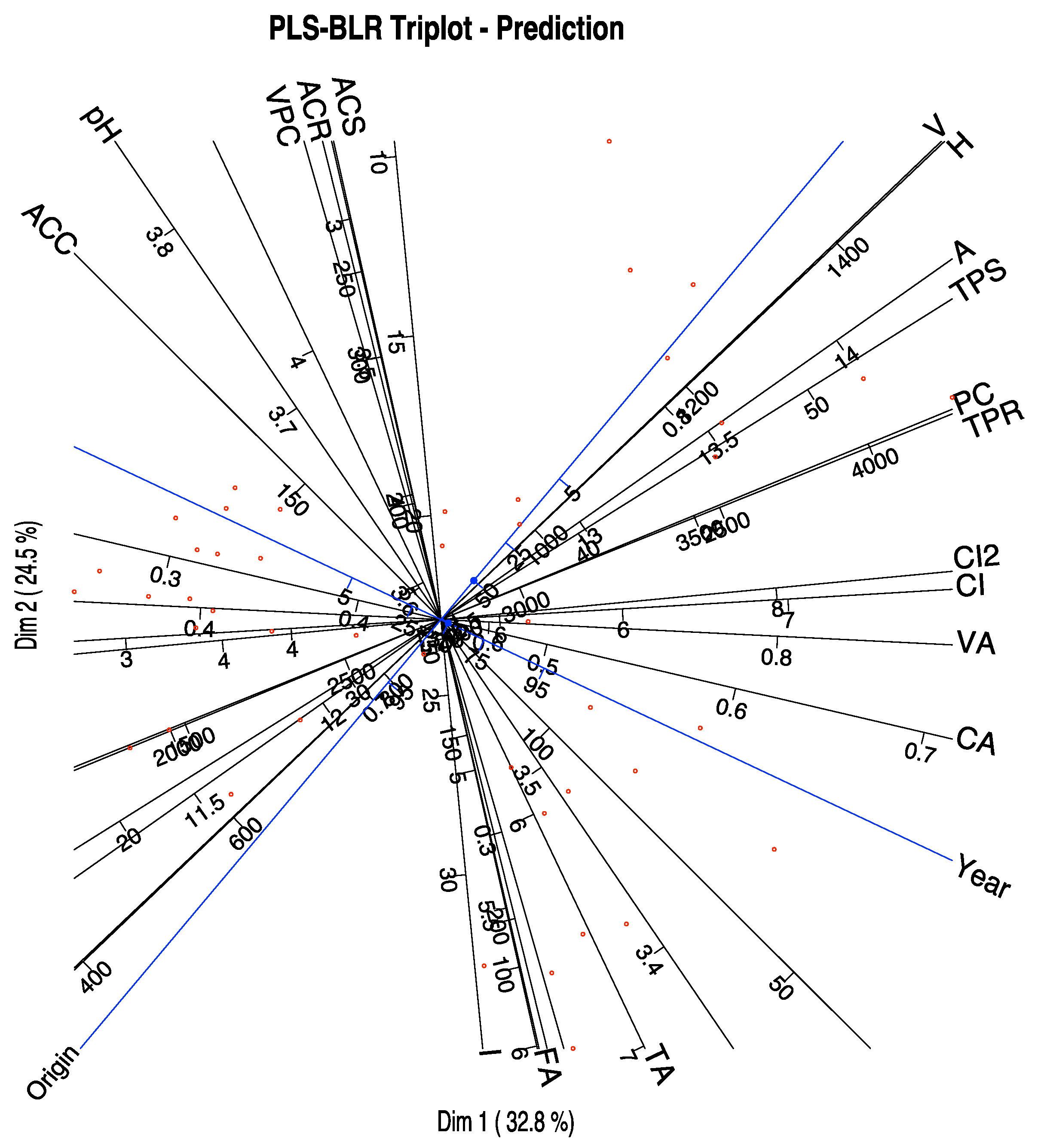
The graphical representation of the first two dimensions is shown in Figure 5. The plot includes not only the predictors but also the responses.

Table 3. Fit measures for each response.

	Deviance	D.F	p-Val	Nagelkerke	Cox-Snell	MacFaden	% Correct
Year	40.3754	2	0.0000	0.7930	0.5923	0.6530	86.6667
Origin	16.4241	2	0.0003	0.4556	0.3058	0.3281	93.3333
Total	56.7995	4	0.0000	0.6577	0.4680	0.5077	90.0000

shows some measures of the quality of representation for the binary variables, including a test for the comparison with the null model, three pseudo R-squared measures and the percent of correct classifications.

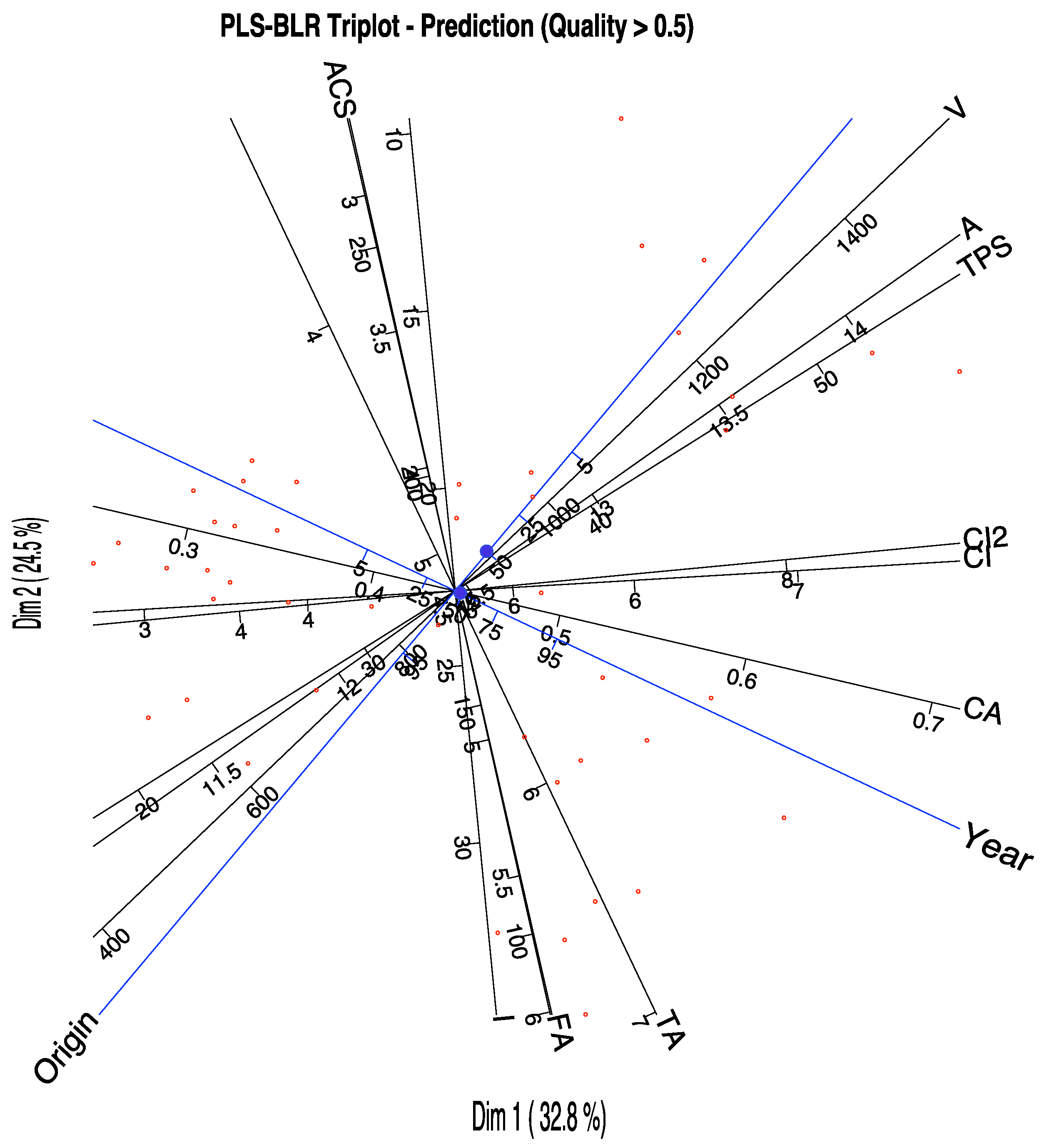
The picture can help in the identification of the most important variables for the prediction. We can select on the graph only the variables with high qualities of representation, for example higher than 0.6. (Figure 6). The actual qualities are in

Table 4. Cumulative qualities of the columns (percent of the variability of the variable accounted for the first dimension and the sum of the first two).

	Component 1	Components 1 + 2
A	56.40	83.02
VA	33.13	32.96
TA	16.32	65.46
FA	5.15	78.39
pH	14.50	34.87
TPR	48.85	57.54
TPS	58.48	80.88
V	33.20	60.38
PC	48.21	57.11
ACR	2.13	26.96
ACS	4.46	65.60
ACC	32.76	52.63
CI	67.69	68.43
CI2	67.17	68.51
H	16.11	29.14
I	1.00	78.30
CA	83.77	84.44
VPC	0.74	7.11

.

We can have a simpler graph removing the scales for each variable and changing the lines by vectors as in Figure 7. The scales may be useful when we want to know the approximate values of the variables for each wine or group of wines, but for a general interpretation, the last graph is also useful and more readable. The software package allows for the selection of variables to represent to clean the final picture. That is intended to explore the triplot on the computer screen, but it is sometimes difficult to do the same in the limited space of a piece of paper.

The variables that better predict the responses are those with higher qualities, in order, Chemical Age (CA), Alcoholic content (A), Total phenolics-Somers (TPS), Fixed acidity (FA), Degree of Ionization (I), Colour density (CI & CI2), Total Anthocyanins (ACS), Total titratable acidity (TA), Substances reactive to vanillin (V), Total phenolics-Folin (TPR), Procyanidins (PC) and Malvidin (ACC).

A closer inspection of the graphic shows that VA, A, TPS, PC and TPR are more closely related to the Origin and are higher in Toro. Variables CA and ACC are related to the Year, the first being higher in 1986 and the second in 1987. The variables CI and CI2 that are actually two measures of the colour are somewhat associated to both Origin and Year, being higher for the wines of Toro in the first year. ACS is associated to the second year, and Toro and FA and TA with the first year and Ribera de Duero.

In summary, Toro wines are darker, with higher alcohol content, higher phenolics and procyanidins, in comparison to the Ribera de Duero wines. Color also changes with the year as well as the chemical age and malvidins. Anthocyanins and acidity change with both origin and year.

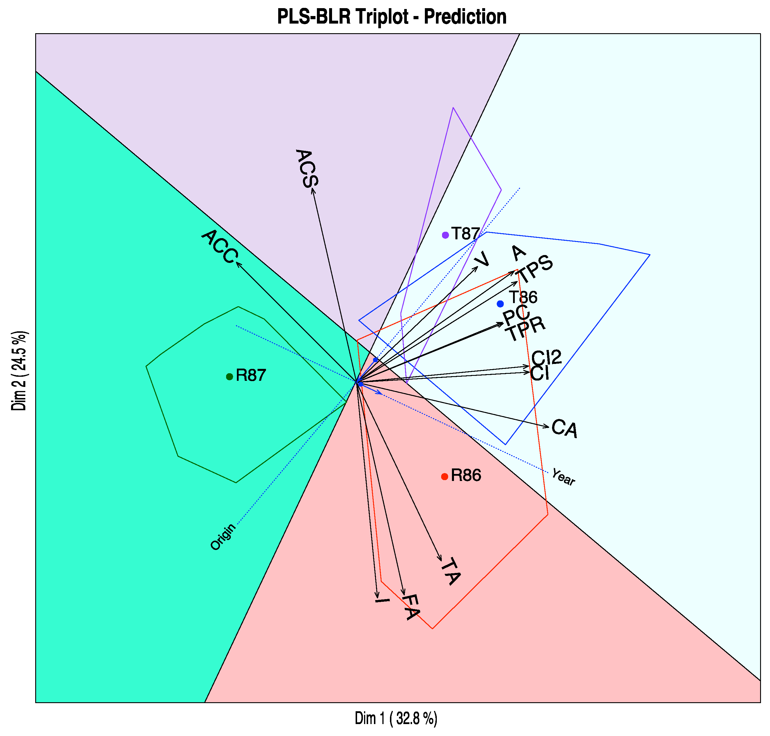
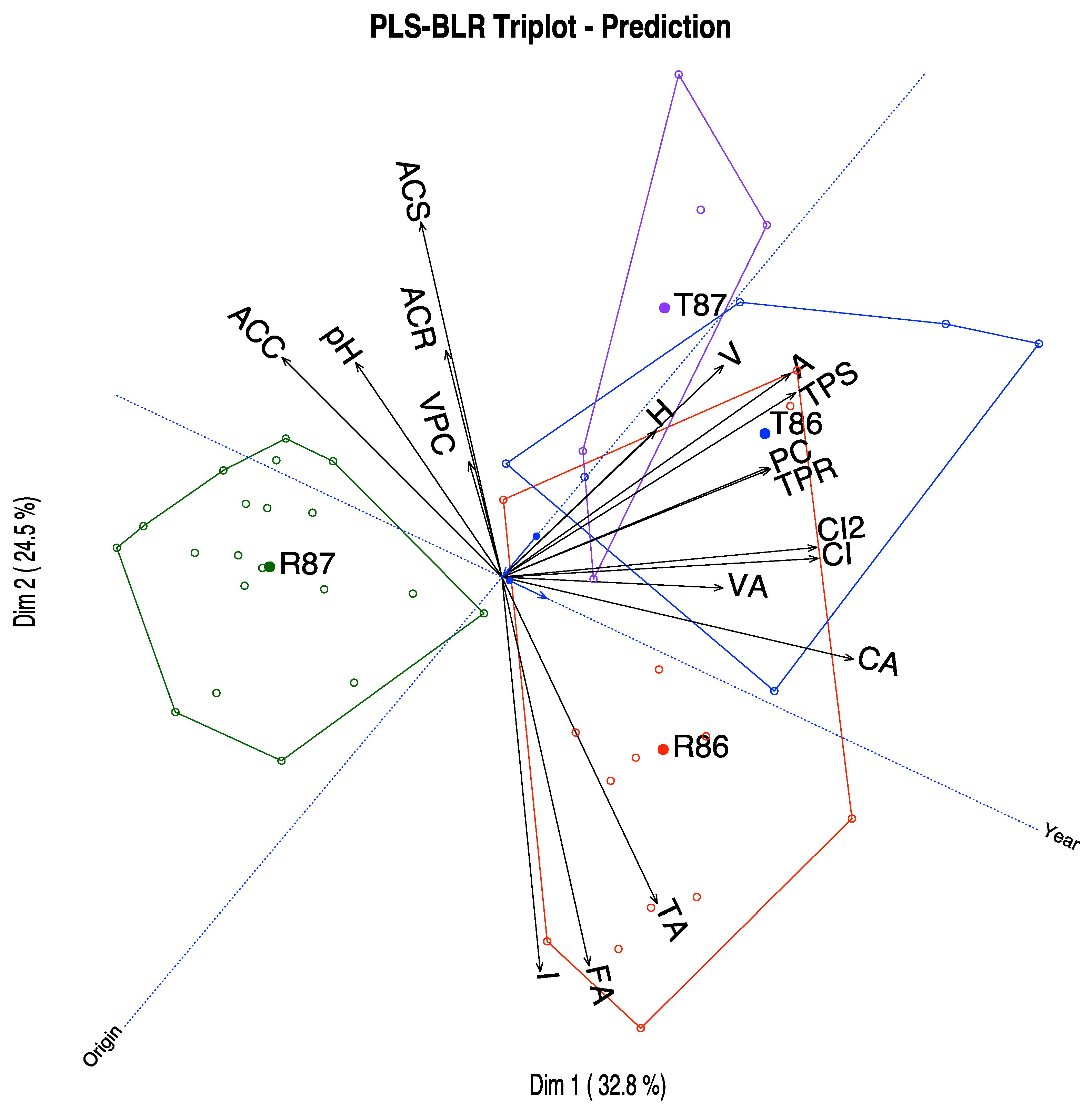
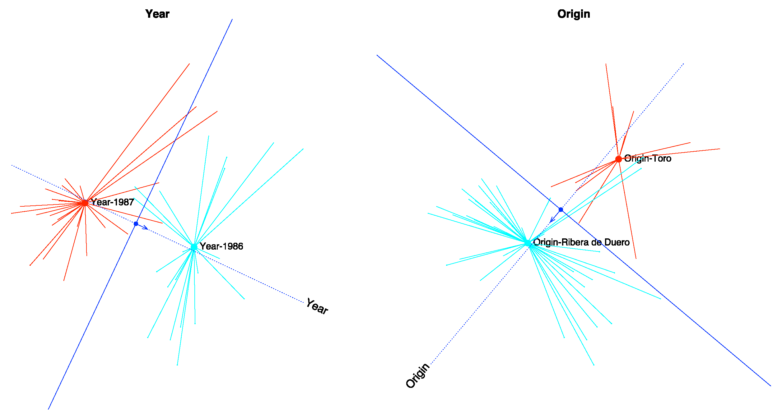
We obtain 90% of correct classifications, 86.67% for the year and 93.33% for the origin respectively. Together with the values of the pseudo $R^2$, we can state that the prediction is accurate (See Table 3). We can check that graphically in Figure 8 where the dotted lines are the directions that best predict the probability, the arrows show the direction of increasing probabilities and the perpendicular line the limits of the prediction region. The arrows start at the points predicting 0.5 and end at the points predicting 0.75. If we classify an individual into a group when the expected probability is higher than 0.5, we can observe that most of the points are on the right prediction region.

Finally, we have placed the convex hulls containing the points for each combination of origin and year as well as the regions that predict the same combinations on the graph. We can see that most of the points lie on the correct prediction region, see Figure 9.

5.2. Spiders Data

As a second example, we have a data set published in [36]. The data have been used by several authors to illustrate different ordination techniques, for example by [37] in its original paper about Canonical Correspondence Analysis.

The original matrix contained the abundances of 12 species of wolf spiders captured at 100 sites (pitfall traps) in an area with dunes in The Netherlands. We have the abundances at 28 sites where a set of environmental variables were also available. The names of the actual species as well as the data tables can be found in [11].

Initial data have been converted into a binary format. Our responses will be presences or absences of the spider species. Our predictors are a set of six environmental variables measured at the same sites that may explain the presence or absence of the species. Names of the variables as well as the data tables can also be found in [11].

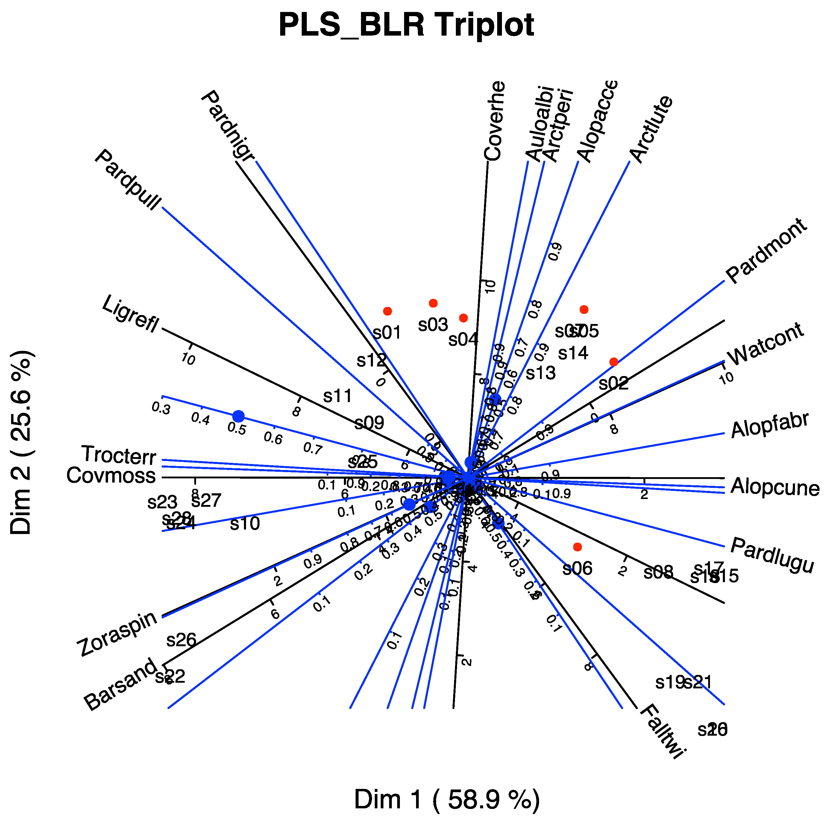
Components for the predictors are the linear combinations of the variables that better predict the presence and absence of the species. Both species and environmental variables are represented together on the same biplot.

Table 5. Explained variance.

	Eigenvalue	Exp. Var	Cumulative
Comp. 1	95.44	58.91	58.91
Comp. 2	41.49	25.61	84.53

contains the amount of variability of the environmental data explained by the PLS components. The first two dimensions explain an 84.53% of the variance.

In this analysis, all the environmental variables are well represented. The qualities are shown in

Table 6. Qualities of the columns.

	Comp. 1	Comp. 2
Watercontent	92.52	90.44
Baresand	70.95	71.87
Covermoss	66.20	66.22
Ligthrefl	79.35	97.13
Falltwings	43.65	93.61
Coverherbs	0.82	87.90

.

The information for the fit of the responses is in

Table 7. Measures of fit for the spider data.

	Deviance	D.F	p-Val	Nagel.	Cox-Sn.	MacF.	% Correct	Sensit.	Specif.
Alpac	11.89	2	0.00	0.51	0.35	0.38	85.71	85.71	85.71
Alopcu	12.47	2	0.00	0.49	0.36	0.33	85.71	82.35	90.91
Alopfa	17.65	2	0.00	0.63	0.47	0.47	89.29	88.24	90.91
Arctlu	14.46	2	0.00	0.54	0.40	0.37	71.43	73.33	69.23
Arctpe	20.06	2	0.00	0.68	0.51	0.52	85.71	78.57	92.86
Auloal	18.73	2	0.00	0.65	0.49	0.49	85.71	83.33	87.50
Pardlu	0.54	2	0.77	0.05	0.02	0.04	85.71	84.62	100.00
Pardmo	13.71	2	0.00	0.54	0.39	0.39	89.29	94.74	77.78
Pardni	8.12	2	0.02	0.37	0.25	0.26	85.71	85.71	85.71
Pardpu	32.50	2	0.00	0.93	0.69	0.87	96.43	100.00	90.91
Trocte	18.01	2	0.00	0.64	0.47	0.48	85.71	90.91	82.35
Zorasp	16.05	2	0.00	0.68	0.44	0.55	89.29	100.00	86.36
Total	184.18	24	0.00	0.60	0.42	0.45	86.31	86.81	85.71

. Most species have a good percentage of correct classifications. The pseudo $R^2$ coefficients are acceptable except for the Pardosa lugubris species. This may be due to the fact that it is present in most of the sites, and then it does not have any discriminant power.

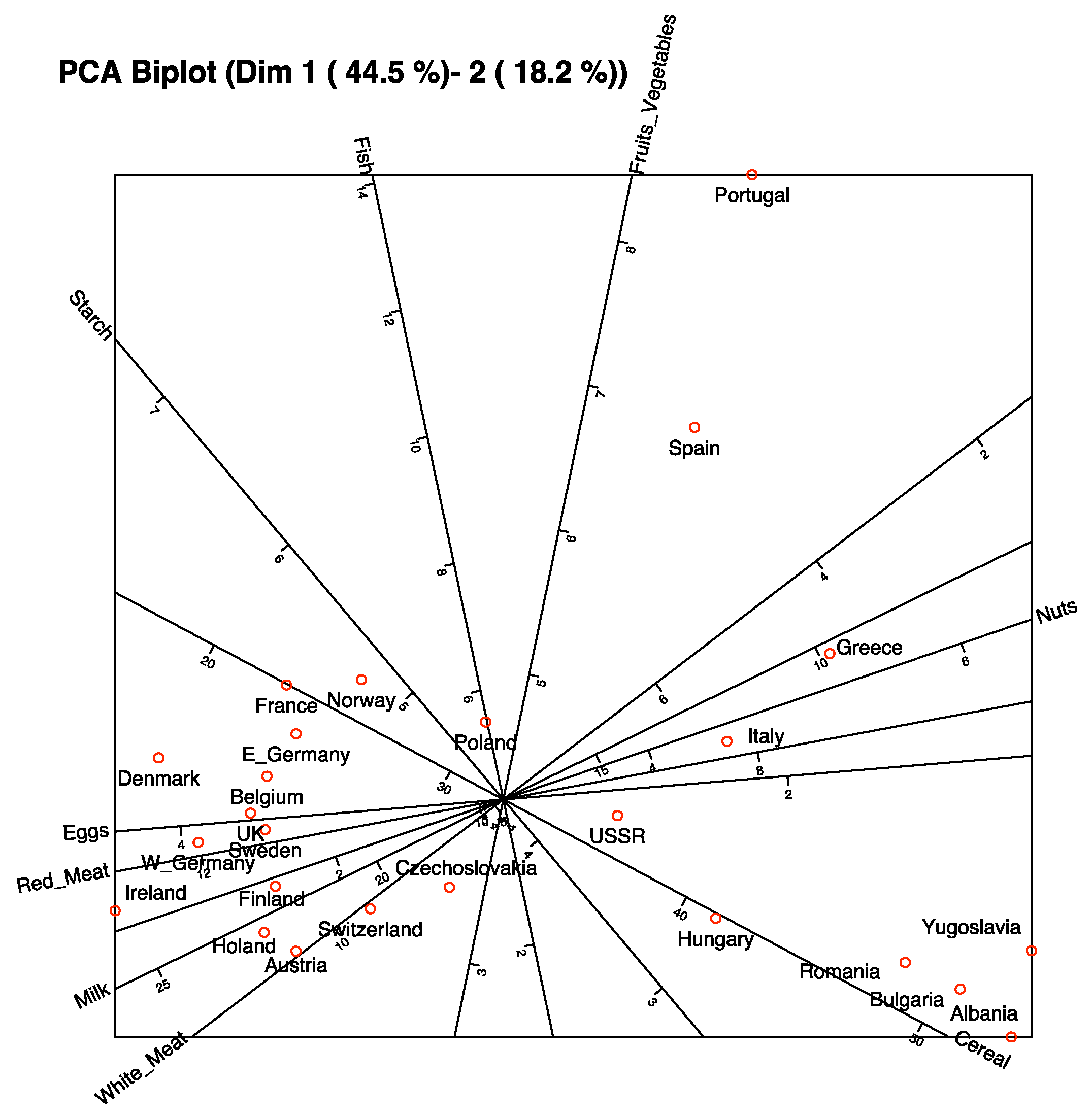
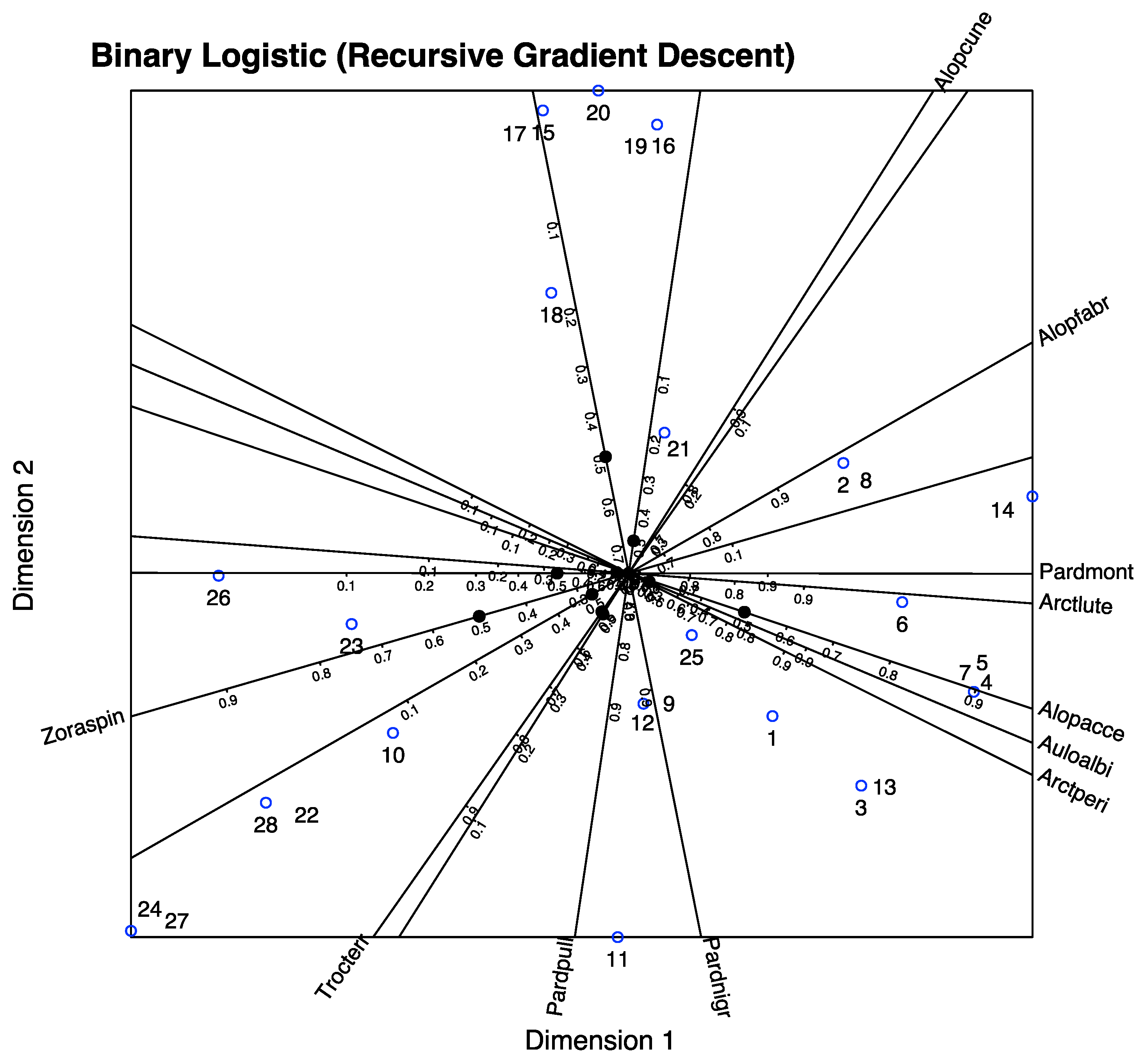
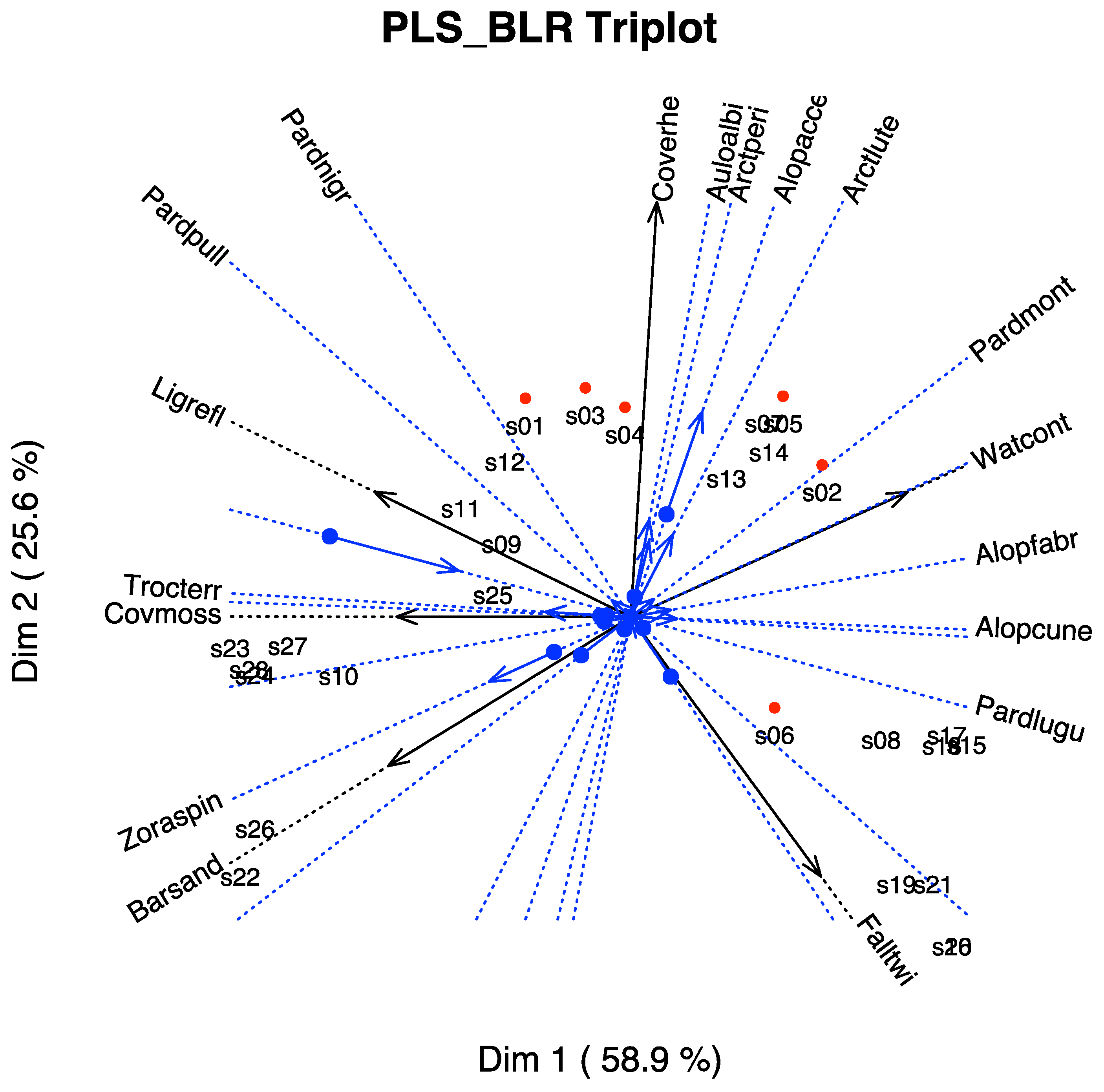
In Figure 10, we have the biplot representation for the spiders data. We have three sets of markers: for the responses (spider species), for the predictors (environmental variables) and for the individuals (sampling sites). A simplified version with arrows nis shown in Figure 11. In the graph, we have a whole picture of the problem. The interpretation is similar to the previous case. For example, higher values of Covermoss are associated to a higher presence of Trocterr and a lower presence of Alopcune. A closer inspection of the biplot permits establishing the relations among the predictors and the responses as well as clusters of sites and their main characteristics.

The graph can also be simplified for readability if we do not want to use the scales of the variables. We have extended the directions of the arrows to place the labels outside.

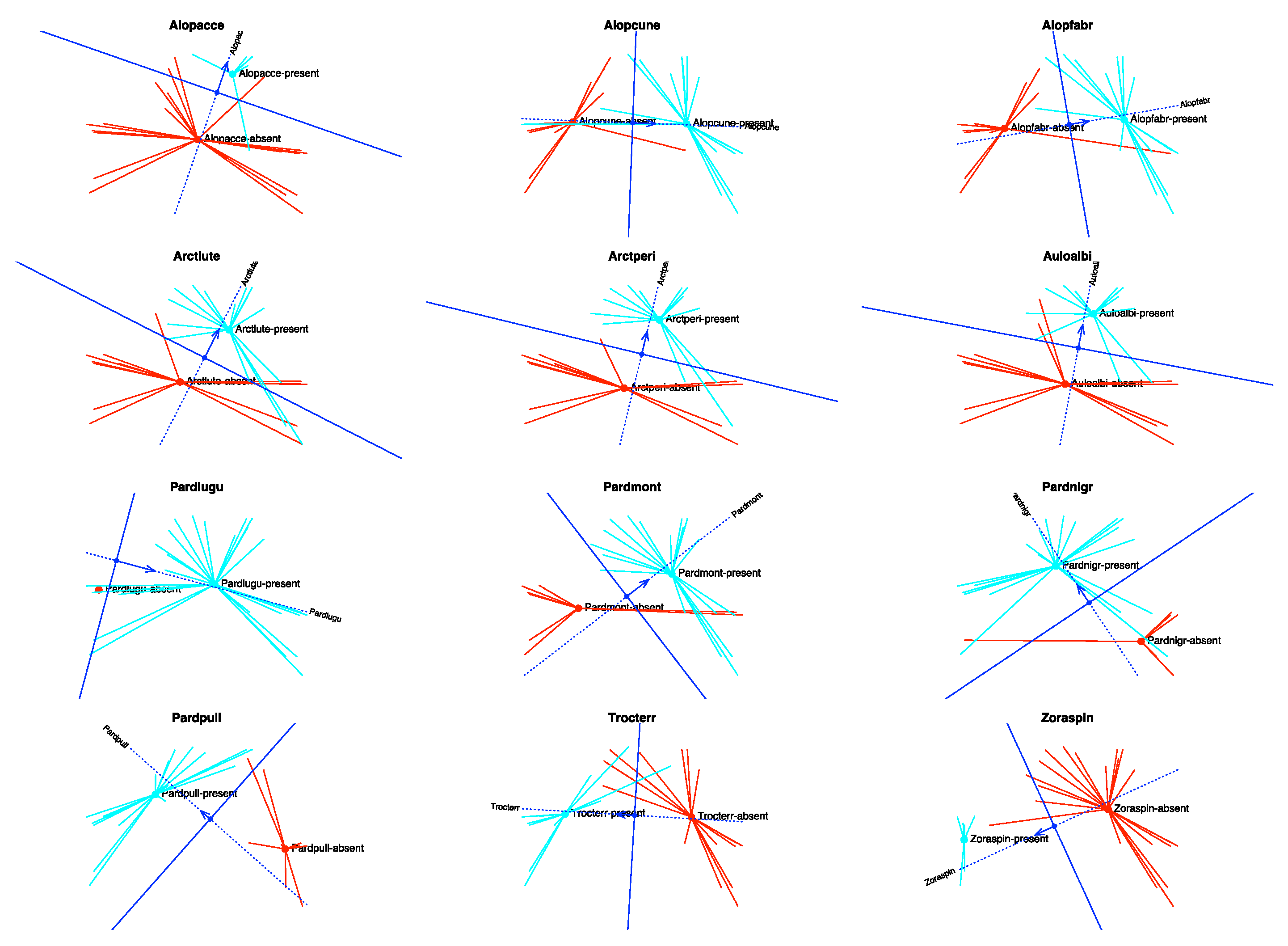
Finally, we show the prediction regions for each response separately (Figure 12). In the graph, the points with observed presences have been represented in blue, the star joins each point with the centroid of the presences. The absences have been coloured in red. As before, the dotted line is the direction that best predicts the expected probability, and the arrow shows the direction of increasing probabilities. The perpendicular line is the separation between the regions predicting presence and absence, the side of the arrow being the prediction of presence.

We can see that most of the observed values lie in the correct prediction regions. This means that the proposed technique correctly captures the structure of the data and the relations among species and environmental variables.

6. Conclusions

In this study, we have proposed a generalization of the PLS-R model to cope with multiple binary responses that was not previously described in the literature. The model is an alternative to PLS-DA using logistic responses rather than the traditional linear models. The difference between them would be similar to the difference between Discriminant Analysis (DA) and logistic regression (LG). It is well known that LR has less restrictions than DA in relation to the distribution of the data.

According to many authors, PLS-R is a very useful method to predict a set of continuous variables from another set of continuous variables, especially when the predictors are highly collinear. PLS-BLR should be useful when the responses are binary, especially when the predictors are wholly collinear or too many for a traditional logistic regression model. This has been proven using the wine data for which the logistic regression do not work properly because of the high collinearity among the variables.

The method developed here is mainly descriptive, and some visualizations have been provided in the form of biplots for each separate set, or triplots, combining both sets of variables (predictors and responses) and the scores for individuals. Biplots and triplots are very useful to interpret the relationships among predictors and responses and to understand the structure of data.

Some further research to establish the significance of the parameters, using resampling methods, will be developed in a near future. In particular, PLS could be extended to nonlinear regression and under Bayesian settings [38].

References

1. Anzanello, M.J.; Fogliatto, F.S. A review of recent variable selection methods in industrial and chemometrics applications. Eur. J. Ind. Eng. 2014, 8, 619–645. [Google Scholar] [CrossRef]
2. Wold, S.; Ruhe, A.; Wold, H.; Dunn, W.J.I. The collinearity problem in linear regression. The partial least squares (PLS) approach to generalized inverses. SIAM J. Sci. Comput. 2006, 5, 735–743. [Google Scholar] [CrossRef] [Green Version]
3. Firinguetti, L.; Kibria, G.; Araya, R. Study of partial least squares and ridge regression methods. Commun. Stat. Simul. Comput. 2017, 46, 6631–6644. [Google Scholar] [CrossRef]
4. Oyedele, O.F.; Lubbe, S. The construction of a partial least-squares biplot. J. Appl. Stat. 2015, 42, 2449–2460. [Google Scholar] [CrossRef]
5. Vargas, M.; Crossa, J.; Eeuwijk, F.A.V.; Ramírez, M.E.; Sayre, K. Using partial least squares regression, factorial regression, and AMMI models for interpreting genotype by environment interaction. Crop Sci. Genet. Cytol. 1999, 39, 955–967. [Google Scholar] [CrossRef]
6. Silva, A.; Dimas, I.D.; Lourenço, P.R.; Rebelo, T.; Freitas, A. PLS Visualization Using Biplots: An Application to Team Effectiveness; Springer Science and Business Media Deutschland GmbH: Berlin/Heidelberg, Germany, 2020; Volume 12251, pp. 214–230. [Google Scholar] [CrossRef]
7. Barker, M.; Rayens, W. Partial least squares for discrimination. J. Chemom. 2003, 17, 166–173. [Google Scholar] [CrossRef]
8. Bastien, P.; Vinzi, V.E.; Tenenhaus, M. PLS generalised linear regression. Comput. Stat. Data Anal. 2005, 48, 17–46. [Google Scholar] [CrossRef]
9. Vicente-Villardon, J.L.; Galindo-Villardón, P.; Blazquez-Zaballos, A. Logistic biplots. In Multiple Correspondence Analysis and Related Methods; Greenacre, M., Blasius, J., Eds.; Statistics in the Social and Behavioral Sciences; Chapman & Hall/CRC: Boca Raton, FL, USA, 2006; pp. 503–521. [Google Scholar]
10. Demey, J.R.; Vicente-Villardon, J.L.; Galindo-Villardón, M.P.; Zambrano, A.Y. Identifying molecular markers associated with classification of genotypes by External Logistic Biplots. Bioinformatics 2008, 24, 2832–2838. [Google Scholar] [CrossRef] [PubMed] [Green Version]
11. Vicente-Villardon, J.L.; Vicente-Gonzalez, L. Redundancy analysis for binary data based on logistic responses. In Data Analysis and Rationality in a Complex World; Chadjipadelis, T., Lausen, B., Markos, A., Lee, T., Montanari, A., Nugent, R., Eds.; Studies in Classification, Data Analysis, and Knowledge Organization; Springer International Publishing: Berlin/Heidelberg, Germany, 2021; pp. 331–339. [Google Scholar] [CrossRef]
12. Wold, H. Soft modelling by latent variables: The non-linear iterative partial least squares (NIPALS) approach. J. Appl. Probab. 1975, 12, 117–142. [Google Scholar] [CrossRef]
13. Wold, S.; Esbensen, K.; Geladi, P. Principal component analysis. Chemom. Intell. Lab. Syst. 1987, 2, 37–52. [Google Scholar] [CrossRef]
14. Golub, G.; Van Loan, C. Matrix Computations; Johns Hopkins Studies in the Mathematical Sciences, Johns Hopkins University Press: Baltimore, MD, USA, 2013. [Google Scholar]
15. Andrecut, M. Parallel GPU implementation of iterative PCA algorithms. J. Comput. Biol. 2009, 16, 1593–1599. [Google Scholar] [CrossRef] [PubMed] [Green Version]
16. Babativa-Márquez, J.G.; Vicente-Villardon, J.L. Logistic biplot by conjugate gradient algorithms and iterated SVD. Mathematics 2021, 9, 2015. [Google Scholar] [CrossRef]
17. Albert, A.; Anderson, J.A. On the existence of maximum likelihood estimates in logistic regression models. Biometrika 1984, 71, 1–10. [Google Scholar] [CrossRef]
18. Heinze, G.; Schemper, M. A solution to the problem of separation in logistic regression. Stat. Med. 2002, 21, 2409–2419. [Google Scholar] [CrossRef]
19. le Cessie, S.; van Houwelingen, J.C. Ridge estimators in logistic regression. J. R. Stat. Soc. Ser. C Appl. Stat. 1992, 41, 191–201. [Google Scholar] [CrossRef]
20. Kiers, H.A. Setting up alternating least squares and iterative majorization algorithms for solving various matrix optimization problems. Comput. Stat. Data Anal. 2002, 41, 157–170. [Google Scholar] [CrossRef]
21. Gabriel, K.R. The biplot graphic display of matrices with application to principal component analysis. Biometrika 1971, 58, 453–467. [Google Scholar] [CrossRef]
22. Gower, J.; Hand, D. Biplots; Chapman & Hall/CRC Monographs on Statistics & Applied Probability, Taylor & Francis: Abingdon, UK, 1995. [Google Scholar]
23. Hand, D.J.; Daly, F.; McConway, K.; Lunn, D.; Ostrowski, E. A Handbook of Small Data Sets; CRC Press: Boca Raton, FL, USA, 1993; p. 458. [Google Scholar]
24. Gabriel, K. Biplot display of multivariate matrices for inspection of data and diagnosis. In Interpreting Multivariate Data; Barnet, V., Ed.; John Wiley and Sons: Hoboken, NJ, USA, 1981; pp. 147–173. [Google Scholar]
25. Benzécri, J.P. L’Analyse des Données; Dunod: Paris, France, 1973; Volume 2. [Google Scholar]
26. Greenacre, M.J. Theory and Applications of Correspondence Analysis, 3rd ed.; Academic Press Inc. Ltd.: London, UK, 1984. [Google Scholar]
27. Gardner-Lubbe, S.; Roux, N.J.L.; Gowers, J.C. Measures of fit in principal component and canonical variate analyses. J. Appl. Stat. 2008, 35, 947–965. [Google Scholar] [CrossRef]
28. Hernández-Sánchez, J.C.; Vicente-Villardón, J.L. Logistic biplot for nominal data. Adv. Data Anal. Classif. 2017, 11, 307–326. [Google Scholar] [CrossRef] [Green Version]
29. Vicente-Villardón, J.L.; Hernández-Sánchez, J.C. External logistic biplots for mixed types of data. In Advanced Studies in Classification and Data Science; Imaizumi, T., Okada, A., Miyamoto, S., Sakaori, F., Yamamoto, Y., Vichi, M., Eds.; Studies in Classification, Data Analysis, and Knowledge Organization; Springer: Berlin/Heidelberg, Germany, 2020; pp. 169–183. [Google Scholar]
30. Cox, D.R.; Snell, E.J. Analysis of Binary Data, 2nd ed.; Chapman & Hall/CRC: Boca Raton, FL, USA, 1970; Volume 7. [Google Scholar] [CrossRef]
31. Nagelkerke, N.J.D. A note on a general definition of the coefficient of determination. Biometrika 1991, 78, 691–692. [Google Scholar] [CrossRef]
32. Vicente-Villardon, J.L. MultBiplotR: Multivariate Analysis Using Biplots in R. R Package Version 1.6.14. 2021. Available online: https://cran.r-project.org/web/packages/MultBiplotR/index.html (accessed on 20 July 2022).
33. Nash, J.C. Optimr: A Replacement and Extension of the ‘optim’ Function. R Package Version 12.6. 2019. Available online: https://cran.r-project.org/web/packages/optimr/index.html (accessed on 20 July 2022).
34. Rivas-Gonzalo, J.C.; Gutiérrez, Y.; Polanco, A.M.; Hebrero, E.; Vicente-Villardon, J.L.; Galindo-Villardon, M.P.; Santos-Buelga, C. Biplot analysis applied to enological parameters in the geographical classification of young red wines. Am. J. Enol. Vitic. 1993, 44, 302–308. [Google Scholar]
35. Galindo-Villardón, P. Una alternativa de representación simultánea: HJ-Biplot. Qüestiió Quad. D’estadística I Investig. Oper. 1986, 1, 13–23. [Google Scholar]
36. Aart, P.J.V.D.; Smeenk-Enserink, N. Correlations between distributions of hunting spiders (Lycosidae, Ctenidae) and environmental characteristics in A dune area. Neth. J. Zool. 1974, 25, 1–45. [Google Scholar] [CrossRef]
37. Braak, C.J.T. Canonical correspondence analysis: A new eigenvector technique for multivariate direct gradient analysis. Ecology 1986, 67, 1167–1179. [Google Scholar] [CrossRef] [Green Version]
38. Contreras-Reyes, J.E.; Quintero, F.O.L.; Wiff, R. Bayesian modeling of individual growth variability using back-calculation: Application to pink cusk-eel (Genypterus blacodes) off Chile. Ecol. Model. 2018, 385, 145–153. [Google Scholar] [CrossRef]
Figure 1. Prediction biplot with scale markers for the protein consumption data in European countries.
Mathematics 10 02580 g001
Figure 2. Interpolation biplot with three variables.
Mathematics 10 02580 g002
Figure 3. Typical logistic biplot representation with graded scales for the binary variables. The data used for the biplot are the binary matrix of the second example in the next section.
Mathematics 10 02580 g003
Figure 4. Typical logistic biplot representation with arrows for the binary variables. The data used for the biplot is the binary matrix of the second example in the next section.
Mathematics 10 02580 g004
Figure 5. PLS Prediction Triplot for the wine data.
Mathematics 10 02580 g005
Figure 6. PLS-BLR Triplot for the wine data showing only the variables with a predictiveness higher than 0.6.
Mathematics 10 02580 g006
Figure 7. PLS-BLR Triplot for the wine data with groups represented as convex hulls.
Mathematics 10 02580 g007
Figure 8. Prediction regions for each separate variable.
Mathematics 10 02580 g008
Figure 9. Prediction regions for the combination of both variables.
Mathematics 10 02580 g009
Figure 10. PLS-BLR Triplot for the spider data with scales for the variables.
Mathematics 10 02580 g010
Figure 11. PLS-BLR Triplot for the spider data with arrows.
Mathematics 10 02580 g011
Figure 12. Prediction regions for each species.
Mathematics 10 02580 g012